© Universiti Tun Hussein Onn Malaysia Publisher’s Office
IJIE
Journal homepage: http://penerbit.uthm.edu.my/ojs/index.php/ijie
The International
Journal of
Integrated
Engineering
ISSN : 2229-838X e-ISSN : 2600-7916Prediction of Compressive Strength in High Performance
Concrete with Hooked-End Steel Fiber using K-Nearest
Neighbor Algorithm
Abdulhameed Umar Abubakar
1,*, Maimuna Salisu Tabra
21Department of Civil Engineering,
Modibbo Adama University of Technology, P.M.B. 2076 Adamawa, NIGERIA
2Department of Mathematics,
Gombe State University, P.M.B. 127 Gombe, NIGERIA
*Corresponding Author
DOI: https://doi.org/10.30880/ijie.2019.11.01.016
Received 16 June 2018; 02 January 2019; Available online 30 April 2019
1.
Introduction
Compressive strength, fc of concrete is affected by a number of factors such as type and percentage of cement,
water content, size and amount of additives and aggregates, mixing procedures, and compaction as well as curing process [1], [2]. In concrete with fiber addition, it has been reported that this addition sometimes exert influence on the strength of the resulting concrete. The work of [3], reported that fc of concrete with steel fiber addition increased with
fiber content for lower aspect ratio, while in higher aspect ratio, the increase was up to 1% before it fluctuates. This corresponds to what has been reported in the literature that it can either increase, decrease, or show no trend at all [4], [5]. This trend in concrete with steel fiber addition present a challenge especially when prediction of strength is the ultimate goal, when using machine learning applications. This is because the program has to be trained to be conversant with the dataset to be able to make accurate predictions.
Abstract: In this study, the predictive capability for compressive strength of IBk (Instance-Bases learning with parameter k) a K-Nearest Neighbor algorithm was put to test in high performance concrete (HPC) with steel fiber addition. To achieve this objective, 150 x 300 mm cylindrical specimens were casted at least three for each batch and steel fibers were added from 0.50% - 2.00% at 0.25% interval. The mean and standard deviation were determined, and these were used to generate 100 compressive strength values within this range for each proportion. IBk classifier with K =1 nearest neighbor and 3 split percentages for training and testing were utilized. Results indicate that it is possible to generate good compressive strength results from good mean and standard deviation values. For each of the split percentages, the mean, standard deviation, and standard error of mean were determined and is presented. Compressive strength results for the samples were also presented. The prediction capability was very high using this algorithm with small amount of associated errors. Validation of the model using predicted versus actual results shows a very high correlation coefficient. This result indicates the efficiency of the model and its predictive capacity. It also indicates that this can improve the optimization capacity of HPC mixtures with steel fiber addition.
In machine learning applications, mathematical models are developed to predict a particular response of interest by feeding the algorithm with dataset to train, then test the data for evaluation. This is done to validate the performance of the prediction by using linear regression, neural networks, or support vector regression (SVR).
Artificial Neural Network (ANN) has been successfully used to predict multiple variables and nonlinear behavior of different parameters in concrete mixture to obtain compressive strength under different ages [6], [7].
Some studies [8] designed an ANN model that predict and classify compressive strength in low, moderate, and high strength. This consist of eight (8) attributes and 1030 datasets with three learning scheme ratios for training-to-testing of datasets. They were learning scheme (LS), LS1 (40:60), LS2 (50:50), and LS3 (60:40). The correct prediction rate (CPR) for the training data was 96.31%, while for LS1, LS2, and LS3 were 73.01%, 86.02%, and 85.53% respectively. This study however, did not consider the use of fibers as one of the attributes, neither did it use compressive strength. Instead, the age of the concrete was added as an attribute.
K-Nearest Neighbor (KNN) is another algorithm that has found useful application in statistical methods. It is a non-parametric method in statistics because they do not make explicit assumptions about unknown functions. Instead, they seek an estimate of the function that is close to the data points [9]. It works on the principle of storing data for learning, and finding the prediction that is nearest to the training data. In other to classify an input vector, the K-nearest training data is examined and is assigned to the most occurring class. In this algorithm, increasing the K-values reduces the variance of the result, on the other hand inducing bias in the process.
In mathematical terms, given a positive integer K and a test observation Xo, the KNN classifier first identifies the K points in the training data that are closet to Xo, represented by No. It then estimates the conditional probability for class j as the fraction of points in No whose response value equals j.
(
)
(
)
0
0
1 |
r i
i N
P Y j X X I y j
K
= = =
= (1)Finally, KNN applies Bayes rule and classifies the test observation Xo to the class with the largest probability. For example, if we want to make a prediction of a point of interest, for K = 3, KNN will first identify three observations that are closet to the point of interest. However, as cautioned by James et al. [9], the choice of K has a drastic effect on the KNN classifier. When K = 1, the decision boundary is flexible and finds a classifier with low bias but high variance, but when K grows, the flexibility decreases producing a decision boundary close to linear, corresponding to low variance and high bias classifier [9].
It is on this premise that a model capable of predicting compressive strength of HPC with steel fiber addition having eight attributes has been utilized. A total number of 701 datasets were used, and this was possible by generating data from results of experimental mean and standard deviation. This is because it is difficult to generate that much amount of results from experimental data without the problems of variations creeping in during specimen preparations. It is hoped that the results would give a reasonable prediction with limited percentage error.
2.
Materials
Blast-furnace Slag Cement CEM II/B-S 42.5 N that conforms with ASTM C 595 [10] having a specific gravity of 3.15 and silica fume with 82 % SiO2 content was utilized at 10 % of the cement content. High range water reducer GLENIUM 27 was utilized conforming to ASTM C 494 [11] ether brown in color with a density of 1,023 – 1,063 kg/lt, color content < 0.1 % and alkali content < 3 %. Tap water was utilized which conform to BS EN 1008-02 [12] specification. The use of coarse sand with a fineness modulus of 2.7 – 3.0 has been recommended, and in this study fineness modulus of 3.22 was used. Aggregates used were crushed limestone rock conforming to the specification of ASTM C 33 [13]. Aggregate size ranges from 10 – 12 mm is the best and safe choice for maximum size of aggregates in HPC [14]. This is necessitated by the fact that when it increases, the interface zone becomes more heterogeneous and larger, and smaller aggregates are mostly stronger than larger ones as in most rocks with the elimination of internal defects. In summary, the mix design and the proportion utilized for HPC is presented in Table 1. Properties of the constituent materials (ingredients) can be found elsewhere [15]. Steel fibers used in this study were hooked-end bundled type conforming to ASTM A820 [16] with Seven different percentages added to the HPC as 0.5, 0.75, 1.0, 1.25, 1.50, 1.75, and 2.00% by volume of concrete (39.25, 58.88, 78.50, 98.125, 117.75, 137.38, and 157.01 kg/m3, respectively).
Table 1 - Mix design utilized for HPC in reference specimen
Material Cement Water Coarse (10 mm)
Fine
(5 mm) Silica Fume HRWR*
fc
(MPa)
3.
Experimental Procedures
Mixing operation was done with the fibers which are stacked in a fibrillated bundle of water-soluble glue placed last by distribution in small amount to avoid balling. Curing was based on the specifications of ASTM C192 [17] in the curing room and after 24 hours were demolded and placed in the curing tank until testing date.
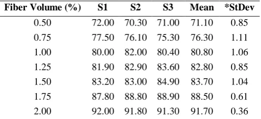
Concrete compressive strength was tested at age of 28 days in accordance with ASTM C39 [18] using 150 x 300 mm cylinders at a loading rate of 0.5 MPa/s. Three cylindrical specimens were prepared for each fiber proportion, and tested at the age of 28 days. The results presented in Table 2 together with the mean and standard deviation.
Table 2 - Compressive strength results for cylinders
Fiber Volume (%) S1 S2 S3 Mean *StDev 0.50 72.00 70.30 71.00 71.10 0.85 0.75 77.50 76.10 75.30 76.30 1.11 1.00 80.00 82.00 80.40 80.80 1.06 1.25 81.90 82.90 83.60 82.80 0.85 1.50 83.20 83.00 84.90 83.70 1.04 1.75 87.80 88.80 88.90 88.50 0.61 2.00 92.00 91.80 91.30 91.70 0.36 *StDev = Standard Deviation
4.
Prediction Methodology
The algorithm utilized was IBk, a K-Nearest Neighbor (KNN) classifier algorithm which is a free open source Java based application in Weka Software created by University of Waikato, New Zealand. One (K = 1) nearest neighbor was used, with eight attributes (cement, water, coarse, fine, silica fume, high range water reducer, steel fiber, and compressive strength).
A total of 701 data sets were utilized generated from Table 2. For this purpose, the mean and standard deviation of each fiber addition level was used to generate 100 random values within the mean and the standard deviation using Minitab 17 software. This was done by going to “Calc” in the menu bar, followed by “Random Data”, then “Normal” for normally distributed data. We then specified the number of rows (100), mean and the standard deviation. Subsequently, the same procedure was done for the other fiber addition levels. Data produced can be found in the appendix.
Input data for the software was prepared in the form of ‘arff’ format in Notepad, and the attributes defined. All the 701 data for the attributes were placed, each separated by a ‘comma’. In the “Classify” function of the software, “Percentage Split” for training-to-testing of the data was selected as 50-50, 60-40, and 70-30, where some portion of the data was used for training, and the rest for testing. Results were stored in csv format, and it can also be opened in the form of excel spreadsheet.
5.
Results and Discussion
Results obtained from Table 2 were used to generate additional data. In order to verify the accuracy and suitability of the data generated, normality test had to be conducted, and this was done with Minitab 17 Statistical Software. In
Fig.1(a) to Fig. 1(g), it could be seen that the P-value was above 0.05, and the dataset were all swirling around the ‘ideal’ probability distribution line. This is an indication that all were within the 95 % Confidence Interval of the distribution with a good fit. A consequence of the high P-value results in relatively low Anderson-Darling value.
In Table 3, Basic statistical results are presented from the data generated in the appendix for the different fiber addition levels. As a result of the low value of the standard deviation from Table 2 for the respective fiber addition levels, it could be seen that the standard error of the mean was relatively lower, with the exception of 0.75 % and 1.00 % which had a higher standard deviation. This is due to the variation in the results obtained from the average laboratory samples. Calculated standard deviation for the generated samples (N = 100) is also presented having a similar trend as observed in Standard Error of Mean. Also presented is the maximum and minimum value of the samples.
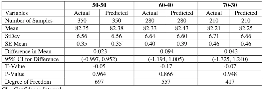
Mean Absolute Error (MAE) which measures the average errors in the prediction stood at 0.64 – 0.68, the Root Mean Squared Error (RMSE) which is the difference between the sample and the prediction, which also is in the range of 0.82 – 0.86. The aim of the prediction is to determine the mean value of compressive strength, and in Table 5 a statistical analysis on the mean difference of the model was conducted. This will show if there is significant difference between the experimental (actual) and the predicted values. At a 95 % CI, the values of the mean difference are presented, and for the three percentage level of splits, all fall within the confidence interval. Also, the P-value at an alpha value of 0.05 shows that they were all above this level.
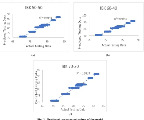
Another way of evaluating the the performance of a model is by measuring the R2 of predicted versus actual values. In Fig. 2(a) to Fig. 2(c), the result of predicted against experimental values is plotted and presented. It could be seen that the coefficient of determination for all is at 98%, which shows a strong positive correlation.
(a) (b)
(c) (d)
(g)
Fig. 1- Normality test for the generated data
Table 3 - Basic statistics
Variable 0.50% 0.75% 1.00% 1.25% 1.50% 1.75% 2.00%
Samples (N) 100 100 100 100 100 100 100
Mean 71.089 76.243 80.923 82.877 83.711 88.548 91.720
SE Mean 0.0853 0.102 0.116 0.0885 0.0969 0.0592 0.0383
StDev 0.853 1.017 1.164 0.885 0.969 0.592 0.383
Minimum 69.068 74.064 77.780 80.550 81.577 87.115 90.516
Median 71.103 76.205 80.961 82.901 83.779 88.494 -
Maximum 72.791 78.483 83.856 85.208 86.373 89.747 92.607
Table 4 - Model summary for training-to-testing ratio
IBK
Training-to-Testing Split 50-50 60-40 70-30
Correlation Coefficient 0.992 0.992 0.9916
Mean Absolute Error 0.6503 0.6434 0.6825
Root Mean Squared Error 0.8296 0.8303 0.8658
Relative Absolute Error (%) 12.2098 12.0701 12.8166
Root Relative Squared Error (%) 12.6324 12.5174 12.9277
Number of Instances 350 280 210
Table 5 - Confidence Interval (CI) of the difference in mean for the model
50-50 60-40 70-30
Variables Actual Predicted Actual Predicted Actual Predicted
Number of Samples 350 350 280 280 210 210
Mean 82.35 82.38 82.33 82.43 82.21 82.25
StDev 6.56 6.56 6.64 6.60 6.71 6.66
SE Mean 0.35 0.35 0.40 0.39 0.46 0.46
Difference in Mean -0.023 -0.094 -0.043
95% CI for Difference (-0.997, 0.952) (-1.194, 1.005) (-1.325, 1.240)
T-Value -0.05 -0.17 -0.07
P-Value 0.964 0.866 0.948
Degree of Freedom 697 557 417
R² = 0.9841
70 75 80 85 90 95
65 75 85 95
Pr
ed
icte
d
Te
sti
n
g
D
ata
Actual Testing Data
IBK 50-50
R² = 0.9845
70 80 90 100
65 75 85 95
Pr
e
d
icte
d
Te
sti
n
g
D
a
ta
Actual Testing Data
IBK 60-40
(a) (b)
(c)
Fig. 2 - Predicted versus actual values of the model
6.
Summary
This study evaluated the prediction of compressive strength of HPC with steel fiber using KNN algorithm, and the following conclusions have been reached:
▪ To be able to obtain good results for accurate prediction, the mean of the individual experimental samples has to be close to each other, and the standard deviation small. This can be ensured by strict quality control during the production of the specimens.
▪ It is possible to generate good random sample values that is capable of being utilized for statistical analysis and model prediction from experimental mean and standard deviation under strict quality control.
▪ IBk algorithm can accurately predict the compressive strength of concrete with steel fiber addition from random results generated from experimental results.
▪ The coefficient of determination of the model for the three percentage splits were 99% while in the validation done through predicted versus actual results to be 98%. An indication of the accuracy of the prediction.
References
[1] Neville, A. M. (2005). Properties of concrete (14th ed.) New York: Wiley.
[2] Nazerigivi, A., Nejati, H. R., Ghazvinran, A., and Najigivi, A. (2017). Influence of nano-silica on the failure mechanism of concrete specimens. Computers and Concrete, 19(4), 427-432.
[3] Abubakar, A. U. (2018). Influence of steel fiber addition on workability and mechanical behavior of high performance concrete, PhD Thesis. EMU North Cyprus.
[4] Traina, L. A., and Mansour, S. A. (1991). Biaxial strength and deformational behavior of plain and steel fiber concrete. ACI Materials Journal, 88, 354-364.
[6] Duan, Z. H., Kou, S. C., and Poon, C. S. (2013). Prediction of compressive strength of recycled aggregate concrete using artificial neural networks. Construction and Building Materials, 40, 1200-1206.
[7] Chou, J. S. C., and Tsai, C. F. (2012). Concrete compressive strength analysis using a combined classification and regression technique. Automation in Construction, 24, 52-60.
[8] Khashman, A., and Akpinar, P. (2017). Non-destructive prediction of concrete compressive strength using neural networks. Procedia Computer Science, 108C, 2358-2362.
[9] James, G., Witten, D., Hastie, T., and Tibshirani, R. (2017) An introduction to statistical learning: With application in R. Springer Texts in Statistics.
[10] American Society for Testing and Materials (2017). Standard specification for blended hydraulic cement. West Conshohocken: ASTM C595 :2017.
[11] American Society for Testing and Materials (2017). Standard specification for chemical admixtures for concrete. West Conshohocken: ASTM C494 :2017.
[12] British Standard Institution (2002). Mixing water for concrete: Specification for sampling, testing and assessing the suitability of water, including water recovered from processes in the concrete industry, as mixing water for concrete. London: BS EN 1008 :2002.
[13] American Society for Testing and Materials (2016). standard specification for concrete aggregates. West Conshohocken: ASTM C33 :2016.
[14] Aitcin, P. C. (1998). High-performance concrete. New York: E & FN Spon.
[15] Abubakar, A. U., Akcaoglu, T., and Marar, K. (2018). P-value significance level test for high-performance steel fiber concrete (HPSFC). Computers and Concrete, 21(5), 485-493.
[16] American Society for Testing and Materials (2011). Standard specification for steel fibers for fiber reinforced concrete. West Conshohocken: ASTM A820 :2011.
[17] American Society for Testing and Materials (2016). standard practice for making and curing concrete test specimens in the laboratory. West Conshohocken: ASTM C192 :2016.
[18] American Society for Testing and Materials (2018). Standard test method for compressive strength of cylindrical concrete specimens. West Conshohocken: ASTM C39 :2018.
Appendix
Appendix 1 - Generated compressive strength
S/No 0.50% 0.75% 1.00% 1.25% 1.50% 1.75% 2.00%
1 72.47 76.55 81.69 83.46 84.28 87.88 91.72
2 69.66 77.66 81.69 83.5 82.87 88.67 92.39
3 69.25 75.44 82.49 82.95 84.85 89.06 91.93
4 70.63 75.64 81.46 82.05 83.9 88.25 91.83
5 71.4 75.8 78.91 83.32 84.02 88.45 91.33
6 71.84 74.07 81.87 83.18 85.66 88.27 92.05
7 72 77.02 81.5 81.85 83.53 89.39 91.74
8 71.56 76.14 80.44 84.12 83.64 88.14 91.41
9 71.41 76.65 80.91 82.66 84.07 89.05 91.67
10 71.39 74.56 79.6 82.25 81.91 88.76 92.61
11 70.55 74.78 80.11 82 83.49 88.12 91.65
12 70.57 78.47 80.55 82.95 84.77 88.73 91.78
13 70.02 76.15 79.49 83.04 82.96 88.75 91.49
14 72.8 77.17 79.96 83.74 82.52 87.82 91.8
15 71.01 74.67 80.58 82.96 83.32 89.33 91.49
16 70.53 77.19 82.29 82.6 83.97 88.56 91.27
17 71.17 74.97 80.99 83.32 83.2 89.2 91.29
18 71.33 77.25 80.33 82.97 83.83 88.4 92.1
19 70.87 77.45 82.7 81.9 84.62 88.93 92.24
20 70.67 77.84 82.7 80.92 81.58 88.09 91.43
21 71.5 75.42 83.27 82.69 83.16 88.49 91.36
22 72.01 77.11 80.62 82.66 83.09 88.3 91.69
23 71.89 76.78 77.79 83.73 83.48 88.72 91.4
24 71.45 77.48 79.17 82.54 84.73 88.2 91.56
25 71.11 75.24 80.82 83.44 82.77 88.23 91.95
26 72.32 76.96 81.95 83.68 81.76 89.46 91.91
28 70.45 75.5 81 83.25 82.65 88.34 91.56
29 70.59 76.5 79.61 83.37 83.87 89.16 91.71
30 71.09 78.49 78.26 82.38 82.96 87.58 91.88
31 71.63 75.79 81.95 83.29 83.41 89.29 91.88
32 69.56 77.67 81.69 82.8 84.03 87.79 91.47
33 70.61 75.05 80.11 83.02 83.82 88.58 92.08
34 71.03 76.45 80.03 81.46 83.45 87.72 92.24
35 72.1 76.93 82.77 83.74 83.88 88.42 91.75
36 71.34 75.78 82.2 84.22 84.02 88.48 92.27
37 71.95 77.85 81.57 81.63 84.58 88.02 91.91
38 71.77 77.26 79.22 82.66 83.78 88.64 91.79
39 70.62 76.83 80.04 82.67 82.04 87.43 90.52
40 72.03 76.75 83.86 81.85 85.26 89.3 91.88
41 71.06 76.96 80.54 82.62 83.75 89.66 91.81
42 69.99 76.57 79.07 82.7 82.71 88.86 91.99
43 70.41 74.94 81.82 82.81 84.35 88.38 91.88
44 71.11 77.2 82.03 82.2 83.12 89.6 91.27
45 72.18 75.99 79.19 82.17 83.73 88.27 91.6
46 71.7 75.33 81.21 83.58 83.15 88.42 91.67
47 71.75 75.29 80.83 81.8 83.49 88.79 91.4
48 71.87 77.57 80.41 83.85 83.1 89.01 91.89
49 71.71 76.46 80.04 83.23 84.97 88.38 91.33
50 69.08 76.63 80.55 83.51 83.84 88.44 92.04
51 70.89 77.38 79.75 83.52 86.38 89.44 91.31
52 71.29 76.4 81.91 82.11 82.23 87.69 92.08
53 71.55 78.01 79.93 82.64 85.69 88.71 91.62
54 70.9 76.79 81.81 83.58 85.31 87.97 91.81
55 72.09 74.6 81.38 82.74 83.99 88.08 92.06
56 70.91 76.15 79.88 81.83 82.46 87.6 91.45
57 69.15 74.81 81.74 85.21 84.88 88.57 92.53
58 71.11 76.1 81.68 81.5 84.39 88.11 92.04
59 70.8 76.22 80.55 82.87 84.02 88.44 92.05
60 70.98 74.59 82.75 81.7 85.64 87.86 90.89
61 69.64 76.82 80.92 82.11 83.13 88.3 92.53
62 71.17 76.65 81.48 81.53 84.99 88.53 91.88
63 71.18 76.98 81.18 83.51 82.56 88.24 92.14
64 71.69 75.25 80.67 81.97 83.91 88.34 91.54
65 71.03 74.39 80.66 81.52 83.36 88.2 91.66
66 70.7 75.32 81.94 82.68 83.84 88.38 91.92
67 69.07 76.93 80.24 81.76 84.57 88.26 91.95
68 72.61 76.43 82.25 84.25 84.7 88.58 92
69 72.74 75.63 82.57 83.56 83.9 89.64 91.85
70 71.2 75.79 80.68 82.19 83.08 89.1 91.62
71 69.85 75.91 80.58 83.78 82.59 88.5 91.57
72 72.11 75.07 81.5 82.78 84.63 88.75 92.36
73 71.91 75.66 79.46 81.91 84.02 89.27 91.92
74 70.45 75.83 82.17 83.35 84.38 88.14 92.05
75 70.69 76.6 80 81.14 83.06 88.62 90.95
76 69.47 74.99 78.13 82.59 83.89 89.75 92.16
77 71.3 77.77 81.18 84.67 83.79 88.9 91.63
78 70.65 77.58 79.04 83.09 82.75 89.14 91.31
79 70.14 76.77 83.5 84.81 82.15 88.29 91.38
80 70.36 75.99 81.2 80.56 82.01 87.63 91.95
81 70.65 77.4 82.02 83.88 84.09 88.73 90.92
82 71.38 75.92 81.83 82.85 82.43 88.77 91.44
85 69.41 75.67 81.38 84.15 85.43 88.61 91.83
86 72.17 77.02 81.01 82.05 82.98 88.13 91.61
87 70.82 75.26 81.34 82.59 84.38 89.27 91.76
88 71.14 77.07 80.17 83.67 84.91 87.9 91.36
89 71.82 76.86 80.73 83.05 83.17 88.75 90.96
90 71.65 77 80.52 83.12 83.39 87.85 92.27
91 70.22 75.27 81.2 82.59 83.33 87.85 91.4
92 72.67 76.03 81.69 83.92 82.95 89.71 91.26
93 69.92 77.68 80.6 82.49 83.59 88.64 91.17
94 71.89 75.18 80.91 83.15 81.92 89.65 91.73
95 70.8 75.52 81.29 81.28 83.41 87.12 91.77
96 71.02 75.92 81.63 83.77 85.05 89.44 91.64
97 70.64 75.26 79.03 83.72 84.54 89.59 91.36
98 71.65 77.62 81.15 84.24 84.52 87.45 91.92
99 70.98 74.94 80.94 83.38 83.41 88.89 92.15