Learning, Moving, And Predicting With Global Motion Representations

University of Pennsylvania

ScholarlyCommons

Publicly Accessible Penn Dissertations

2018

Learning, Moving, And Predicting With Global

Motion Representations

Andrew Coulter Jaegle

University of Pennsylvania, [email protected]

Follow this and additional works at:

https://repository.upenn.edu/edissertations

Part of the

Artificial Intelligence and Robotics Commons

, and the

Neuroscience and

Neurobiology Commons

This paper is posted at ScholarlyCommons.https://repository.upenn.edu/edissertations/2877

For more information, please [email protected].

Recommended Citation

Jaegle, Andrew Coulter, "Learning, Moving, And Predicting With Global Motion Representations" (2018).Publicly Accessible Penn Dissertations. 2877.

Learning, Moving, And Predicting With Global Motion Representations

Abstract

In order to effectively respond to and influence the world they inhabit, animals and other intelligent agents must understand and predict the state of the world and its dynamics. An agent that can characterize how the world moves is better equipped to engage it. Current methods of motion computation rely on local

representations of motion (such as optical flow) or simple, rigid global representations (such as camera motion). These methods are useful, but they are difficult to estimate reliably and limited in their applicability to real-world settings, where agents frequently must reason about complex, highly nonrigid motion over long time horizons. In this dissertation, I present methods developed with the goal of building more flexible and powerful notions of motion needed by agents facing the challenges of a dynamic, nonrigid world. This work is organized around a view of motion as a global phenomenon that is not adequately addressed by local or low-level descriptions, but that is best understood when analyzed at the low-level of whole images and scenes. I develop methods to: (i) robustly estimate camera motion from noisy optical flow estimates by exploiting the global, statistical relationship between the optical flow field and camera motion under projective geometry; (ii) learn representations of visual motion directly from unlabeled image sequences using learning rules derived from a formulation of image transformation in terms of its group properties; (iii) predict future frames of a video by learning a joint representation of the instantaneous state of the visual world and its motion, using a view of motion as transformations of world state. I situate this work in the broader context of ongoing computational and biological investigations into the problem of estimating motion for intelligent perception and action.

Degree Type

Dissertation

Degree Name

Doctor of Philosophy (PhD)

Graduate Group

Neuroscience

First Advisor

Kostas Daniilidis

Keywords

Computational neuroscience, Computer vision, Deep learning, Machine learning, Motion, Vision

Subject Categories

LEARNING, MOVING, AND PREDICTING WITH GLOBAL MOTION REPRESENTATIONS

Andrew Jaegle

A DISSERTATION

in

Neuroscience

Presented to the Faculties of the University of Pennsylvania

in

Partial Fulfillment of the Requirements for the

Degree of Doctor of Philosophy

2018

Supervisor of Dissertation

Kostas Daniilidis, Ruth Yalom Stone Professor of Computer and Information Science

Graduate Group Chairperson

Joshua I. Gold, Professor of Neuroscience

Dissertation Committee:

Johannes Burge, Assistant Professor of Psychology (Chair)

Diego Contreras, Professor of Neuroscience

Nicole Rust, Associate Professor of Psychology

Jianbo Shi, Professor of Computer and Information Science

ACKNOWLEDGEMENT

I have been privileged to have the support of a fantastic group of colleagues in neuroscience and

computer science during my doctoral studies. I would like to thank my advisor, Kostas Daniilidis,

for his mentorship and encouragement. His intuitions and rigor have been crucial to the development

of the ideas in this dissertation. I would also like to thank Diego Contreras who provided mentorship

and scientific guidance, especially in my first few years at Penn.

I am grateful to the members of both the Daniilidis and Contreras labs. Among many others, Morgan

Taylor, Madineh Sarvestani, Iv´an Fern´andez de Lamo, Stephen Phillips, Daphne Ippolito, Oleh

Rybkin, and Karl Pertsch were the source of countless discussions and inspiration. Thanks to

Ken Chaney and Nikos Kolotouros for computing support. Special thanks to Kosta Derpanis for

consistently providing structure for our discussions and work.

Thanks to the members of my committee, Johannes Burge, Nicole Rust, Jianbo Shi, and Katerina

Fragkiadaki for their advice and encouragement. Thanks to David Brainard and the faculty and staff

associated with the IGERT Complex Scene Perception training grant for creating a space of genuine

interdisciplinary focus. I’m grateful to the members of the Neuroscience Graduate Group, and for

the collaborative and supportive atmosphere the students, faculty, and staff have built.

I had the privilege to spend summers at the Max Planck Institute for Intelligent Systems in T¨ubingen

and at DeepMind in London. I am grateful to my collaborators there, and especially to my hosts:

Michael Black and Javier Romero at the MPI and Greg Wayne at DeepMind. I am grateful to them

for their intellectual generosity.

I am incredibly grateful to my friends and family for providing my life with the structure and

support needed to follow this work through. Thanks to Dave Barack for many fruitful discussions

at the interface of philosophy, neuroscience, and artificial intelligence. Thanks to my bandmate,

John McMillin, for providing me with an outlet for musical creativity. Thanks to my parents and

challenged me to be my best.

This work would not have been possible without the invaluable contributions of collaborators. The

work presented in Chapter 2 was done jointly with Stephen Phillips and Kostas Daniilidis; the

work presented in Chapter 3 was done jointly with Stephen Phillips, Daphne Ippolito, and Kostas

Daniilidis; and the work presented in Chapter 4 was done jointly with Oleh Rybkin, Kosta Derpanis,

ABSTRACT

LEARNING, MOVING, AND PREDICTING WITH GLOBAL MOTION REPRESENTATIONS

Andrew Jaegle

Kostas Daniilidis

In order to effectively respond to and influence the world they inhabit, animals and other intelligent

agents must understand and predict the state of the world and its dynamics. An agent that can

characterize how the worldmoves is better equipped to engage it. Current methods of motion

computation rely on local representations of motion (such as optical flow) or simple, rigid global

representations (such as camera motion). These methods are useful, but they are difficult to estimate

reliably and limited in their applicability to real-world settings, where agents frequently must reason

about complex, highly nonrigid motion over long time horizons. In this dissertation, I present

methods developed with the goal of building more flexible and powerful notions of motion needed by

agents facing the challenges of a dynamic, nonrigid world. This work is organized around a view of

motion as a global phenomenon that is not adequately addressed by local or low-level descriptions,

but that is best understood when analyzed at the level of whole images and scenes. I develop methods

to: (i) robustly estimate camera motion from noisy optical flow estimates by exploiting the global,

statistical relationship between the optical flow field and camera motion under projective geometry;

(ii) learn representations of visual motion directly from unlabeled image sequences using learning

rules derived from a formulation of image transformation in terms of its group properties; (iii) predict

future frames of a video by learning a joint representation of the instantaneous state of the visual

world and its motion, using a view of motion as transformations of world state. I situate this work

in the broader context of ongoing computational and biological investigations into the problem of

Contents

ACKNOWLEDGEMENT . . . iv

ABSTRACT . . . vi

LIST OF TABLES . . . x

LIST OF ILLUSTRATIONS . . . xviii

CHAPTER 1 : Introduction . . . 1

1.1 Overview . . . 1

1.2 Visual motion analysis: local, global, and beyond . . . 2

1.2.1 From local to global motion . . . 3

1.2.2 Motion, representation, and spatiotemporal invariances . . . 7

1.2.3 Designing and learning dynamic representations . . . 10

1.2.4 Motion and prediction . . . 12

1.3 Summary of contents . . . 13

CHAPTER 2 : Fast, robust, continuous monocular egomotion computation . . . 16

2.1 Introduction . . . 16

2.2 Related work . . . 19

2.2.1 Egomotion/visual odometry . . . 19

2.2.2 Continuous, monocular approaches . . . 19

2.2.3 Robust optimization . . . 21

2.3 Problem formulation and approach . . . 22

2.3.1 Visual egomotion computation and the motion field . . . 22

2.3.2 Robust formulation . . . 25

2.3.4 Robust estimation using a lifted kernel . . . 29

2.4 Experiments . . . 31

2.4.1 Evaluation on KITTI . . . 32

2.4.2 Synthetic sequences . . . 34

2.5 Conclusions . . . 35

CHAPTER 3 : Understanding image motion with group representations . . . 37

3.1 Introduction . . . 37

3.2 Related work . . . 39

3.2.1 Motion representations . . . 39

3.2.2 Learning representations using visual structure . . . 40

3.3 Approach . . . 41

3.3.1 Group properties of motion . . . 41

3.3.2 Learning motion by group properties . . . 42

3.3.3 Sequence learning with neural networks . . . 44

3.4 Experiments . . . 45

3.4.1 Rigid motion in 2D . . . 46

3.4.2 Real-world motion in 3D . . . 47

3.5 Conclusion . . . 51

CHAPTER 4 : Predicting the future with transformational states . . . 52

4.1 Introduction . . . 52

4.2 Related work . . . 54

4.3 Approach . . . 57

4.3.1 Transformational states . . . 59

4.3.2 Weighted residual connections . . . 61

4.4 Experiments . . . 63

4.4.1 Datasets . . . 63

4.4.3 Evaluation . . . 67

4.5 Conclusion . . . 69

CHAPTER 5 : Conclusion . . . 71

5.1 Future work . . . 71

5.1.1 Developing functional DNN models of the dorsal stream . . . 71

5.1.2 Long-term prediction for control . . . 73

5.1.3 Discovering degrees of freedom . . . 74

5.1.4 Learning symmetries . . . 75

5.2 Summary . . . 77

APPENDICES . . . 79

A Supplemental material: Fast, robust, continuous monocular egomotion computation 79 A.1 Supplemental experiments . . . 79

A.2 Derivation of linear least squares estimate . . . 82

A.3 Lifted weights formulation . . . 84

A.4 Implementation details of Soatto/Brockett algorithm . . . 84

B Supplemental material: Understanding image motion with group representations . . 90

B.1 Additional Experiments . . . 90

C Supplemental material: Predicting the future with transformational states . . . 94

C.1 Video results . . . 94

C.2 Network architectures . . . 94

C.3 Comparison to other prediction models . . . 99

C.4 Ablation studies . . . 99

List of Tables

TABLE 1 : Average embedding error (equation 3.1) on held-out data. Results are

aver-aged over forward, backward, and loop sequences. Errors are relative to a

chance error of 1: values lower than 1 indicate that equivalent (inequivalent)

motions are close together (far apart) in the embedding space. . . 44

TABLE 2 : Linear regression from the learned embedding to the translation and rotation

of the KITTI odometry dataset consistently performs better than chance

(guessing the mean value). Table entries show mean squared error ±

standard error (percent improvement). . . 47

TABLE 3 : Interpolation distances on KITTI (as in Figure 11), averaged across test

data. Distances are consistently lower for the true frame than for visually

similar frames (inside sequence) and dissimilar frames (outside sequence)

when using the embedding, but not the Euclidean distance. . . 48

TABLE 4 : Comparison of binary cross-entropy (BCE) results (nats/frame) on the

Moving MNIST test set. Lower scores indicate better performance. . . 63

TABLE 5 : Comparison of frame prediction results on the KTH test set. Higher scores

indicate better performance. . . 64

TABLE 6 : Comparison of next frame prediction results on the UCF101 test set (split

1). Higher scores indicate better performance. . . 64

TABLE 7 : Comparison of sequence prediction model components and training

List of Figures

FIGURE 1 : Schematic depiction of the ERL method for egomotion estimation from

noisy flow fields. Figure best viewed in color. (A) Example optical flow

field from two frames of KITTI odometry (sequence 5, images 2358-2359).

Note the outliers on the grass in the lower right part of the image and

scattered throughout the flow field. (B) We evaluate the flow field under

Mmodels with translation parameters sampled uniformly over the unit

hemisphere. The residuals for the flow field under three counterfactual

models are shown. Each black point indicates the translation direction

used. Residuals are scaled to [0,1] for visualization. (C) We estimate the

likelihood of each observed residual under each of the models by fitting a

Laplacian distribution to each set of residuals. The final confidence weight

for each flow vector is estimated as the expected value of the residual

likelihood over the set of counterfactual models. Likelihood distributions

are shown for the three models above. (D) The weighted flow field is

used to make a final estimate of the true egomotion parameters. The black

point indicates the translation direction estimated using ERL and the green

point indicates ground truth. The unweighted estimate of translation is

not visible as it is outside of the image bounds. . . 17

FIGURE 2 : A 2D line-fitting problem demonstrating how ERL weights inliers and

outliers. Inliers are generated asyi≈2xi+1 with Gaussian noise. Each

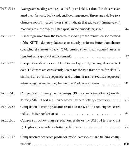
FIGURE 3 : Robust methods recover the error surface of the outlier-free flow field.

(A) Example optical flow field from two frames of KITTI odometry

(sequence 10, images 14-15). Note the prominent outliers indicated by

the yellow box. Error surfaces on this flow field for (A) the raw method

(equation (2.9)) with all flow vectors, (B) with outliers removed by hand,

and (C) with confidence weights estimated by ERL or (D) the lifted

kernel. The green point is the true translational velocity and the black

point the method’s estimate. Blue: low error. Red: high error. Translation

components are given in calibrated coordinates. . . 28

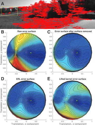
FIGURE 4 : Median translational and rotational errors on the full KITTI odometry

dataset for our methods and baselines. . . 30

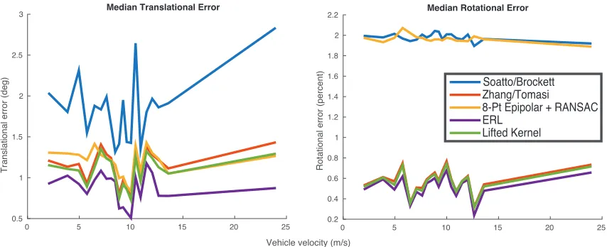
FIGURE 5 : Full distribution of translational velocity errors. . . 33

FIGURE 6 : Full distribution of rotational velocity errors. . . 33

FIGURE 7 : Translation error as a function of percent outliers on synthetic data for our

robust methods and two baseline continuous egomotion methods. . . 35

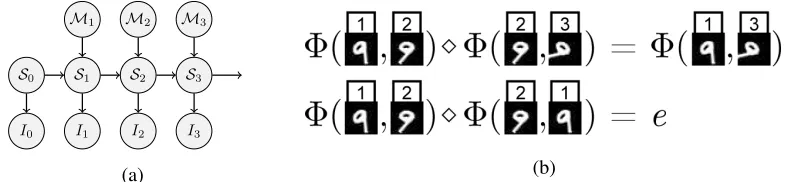
FIGURE 8 : (a)A graphical model describing the relationship between the latent scene

structure_{St}, motion{Mt}, and the observed images of a sequence. We

describe a method for learning a representation_Mof the motion space

Mfrom observed image sequences_{It}.(b)By recomposing sequences

of images to satisfy the group properties of associativity and invertibility,

we construct pairs of image sequences with equivalent motion. We use

these properties to learn an approximate group homomorphismΦ∈ M

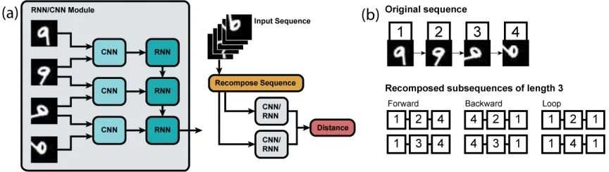
FIGURE 9 : (a)Network structure. The RNN output at the final step of the sequence

is treated as the sequence embedding. During training, the distance

be-tween sequence embeddings is adjusted using an embedding loss.(b)We

recompose sequences to enforce associativity and invertibility. Sequences

with equivalent motion (e.g. 1-2-4 and 1-3-4) serve as positive examples,

while sequences with inequivalent motions (e.g. 1-2-4 and 4-3-1) serve as

negative examples. . . 41

FIGURE 10 : (a)An example test sequence from MNIST and the corresponding saliency

maps. Saliencies show the gradient backpropagated from the final RNN

timestep. Each column represents an image pair passed to one of the

CNNs.(b)-(d)tSNE of the network embedding on the test set, with points

labeled by(b)the magnitude of translation in pixels,(c)the translation

direction in degrees, and(d)the digit label (0-9). The representation

clusters sequences by both translation magnitude and direction but not

FIGURE 11 : (a)Natural image motion is a subspace of the space of all image

trans-formations, and a particular motion can be viewed as a path in the latent

space of natural images. Although [I1,IK,IT] has a total transformation

equivalent to [I1,IT] for any value ofK, only [I1,Im,IT] can be produced

by natural image motion.(b)In interpolation experiments, we compare

the distance between the embedding of [I1, IT] with the embedding of

this sequence after inserting either a true middle frame (Im) or another

frame (IINorIOUT).(c)Images with lowest relative error taken from the

sequence or from the whole dataset, for each distance measure. Errors

are relative to that of the true middle frame in the corresponding measure:

high relative errors ( 1) indicate the distance distinguishes realistic

motion from unrealistic motion. Images other than true middle frame

produce dramatically higher errors when using the embedding but not

when using a Euclidean distance. . . 49

FIGURE 12 : Saliency results on a test sequence from KITTI tracking with both camera

and independent motion. The network focuses on areas that are relevant to

determining motion in 3D, not simply regions with large temporal image

FIGURE 13 : (A) This work is motivated by the observation that image transformations

may be more easily modeled by a network that learns to transform latent

states rather than transform or associate pixel intensities. By learning to

model states,s, along with transformations between states,g, the RNN is

encouraged to model sequences not by memorizing arbitrary transitions

between certain images (static embedding) but by reshaping the

embed-ding so that natural state transformations are predictable (transformational

embedding). Figure best viewed in color. (B) Sample predictions of our

model on sequences from the Moving MNIST and KTH datasets. We show

only the last of 10 input images for visualization purposes. Our model

produces good image predictions using only pixel-wise reconstruction

losses. . . 53

FIGURE 14 : Architecture overview. (A) Our model uses an encoder-decoder

sequence-to-sequence architecture with a factorized latent that captures the image

state,s, and transformation,d. Residual connections are omitted for

clar-ity; see the text and Figure 15 for details. (B) Future states are transformed

from past states using an RNN core that accumulates the transformation

estimategwith a ConvLSTM and applies it to the recursively estimated

FIGURE 15 : Weighted residual connections. (A) To produce high quality images at

multiple time steps in the future without re-encoding images, we use a

residual connection scheme designed to gradually alter image content

from the last observed input image. Residual connections connect the

encoder at timeT (last input) to the decoder at timeT+1 (first output).

At subsequent times, the decoder inherits information about the past from

the decoder at the previous time only. The network has this connectivity

pattern at every layer: we show only two decoder layers and the output

image for easier visualization. (B) We use a retinotopic weighting scheme

to allow each layer of a decoding network to selectively incorporate

skipped input from the past. Weights and feature maps at timet are

functions of the predicted latent state ˆst at timet. . . 60

FIGURE 16 : Example sequences on Moving MNIST. For all three examples, the first

row shows the input sequence (past), the second row shows the ground

truth future, and the third row shows the predicted sequence. Our model

is able to stably predict digits over multiple timesteps, even when digits

overlap for multiple frames. . . 61

FIGURE 17 : Example sequences on KTH. For all three examples, the first row shows

the input sequence (past), the second row shows the ground truth future,

and the third row shows the predicted sequence. The model produces

faith-ful motion in a variety of settings and is able to paint in the background

after dis-occlusion. . . 65

FIGURE 18 : Example sequences on UCF101. For each example, we show two frames

from the past followed by the ground truth third frame and the third frame

FIGURE 19 : Example failure cases on KTH. (a) The model outputs a blurry motion

sequence that does not correspond to the ground truth. (b) The model fails

to correctly predict motion or paint in the background when the moving

object occupies only a small part of the image. (c) The model fails to

correctly paint in the background after the foreground moves, leading to

ghosting artifacts. . . 69

FIGURE 20 : Log likelihoods of Laplacian and Gaussian fits to the optical flow error.

Laplacian fits are consistently better than Gaussian fits. . . 80

FIGURE 21 : Median translational and rotational errors on the full KITTI odometry

dataset for ERL with two candidate distributions. . . 81

FIGURE 22 : Error on egomotion regression from self-supervised flow PCA as a

func-tion of the number of principal components included. Horizontal lines

reflect our method (latent, shown in red) and a chance baseline (show in

green). . . 91

FIGURE 23 : Cumulative percent variance explained of the optical flow in KITTI

odom-etry as a function of the number of principal components included. 67%

of the variance is explained by the first 5 components; 90% of the variance

is explained by the first 40 principal components. . . 92

FIGURE 24 : Representative principal components of optical flow on the KITTI

odom-etry dataset. The first few components capture the dominant motions

(forward and left/right turning) and reflect the stereotypical depth

FIGURE 25 : Comparison of Moving MNIST results on architectures with and without

residual connections. The model labeled “no residuals” has no skip or

residual connections of any kind. The model labeled “w/ residuals” is the

full model described in the paper. The model without weighted residual

connections produces good predictions, but including these connections

produces crisper results, especially at early prediction time steps. Both

architectures reliably capture digit identity, even after the digits overlap. 100

FIGURE 26 : Comparison of KTH results on models with architectural ablations. (i)

“No transformational state”: the RNN core omits the CNNΦand includes

only ConvLSTM components. (ii) “Residuals skipped from last input

image”: each decoder directly receives residual input from the encoder at

the last input time step (t=T) instead of the previous decoder time step.

Weighted residuals are still used. (iii) “No residuals”: no residual or skip

connections of any kind are used. The second sequence shown here is

very challenging for all models. The full model produces better motion

(notice the motion of the legs) and less prominent ghosting artifacts than

ablations. . . 101

FIGURE 27 : Additional comparisons of KTH results on models with architectural

CHAPTER 1 : Introduction

1.1. Overview

The visual world is complex and ever changing, and its complexity extends from local structures to

more extended patterns in space and time. For an intelligent agent to effectively engage the world, it

must learn to reason about how the state of the world is changing, and how local states and changes

reflect the larger patterns and structures of the world.

Visual motion is at the core of these issues, and in this dissertation we develop methods towards the

goal of understanding motion. For an agent to make best use of of motion, it is important that its

representations do not merely reflect the low-level statistics of the world: they should reflect the full

set of properties observable by an agent. Accordingly, I focus on the problem of understanding global

motion. By global motion, I mean the motion of the full image and ultimately the scene, not just

of individual pixels. Understanding motion in this sense will facilitate the development of methods

enabling intelligent agents to use the changes observed in the world to understand it and to act in it.

The body of this dissertation is composed of three works, which develop methods for motion analysis

and motion-based prediction. Before presenting the technical contributions of this dissertation, I

survey the state of motion analysis by reviewing the computational problem of motion analysis, local

approaches to motion and their relationship to global methods, and challenges to the current state of

motion research motivated by the computational goals of prediction and spatiotemporally invariant

representation. In chapters 2, 3, and 4, I present work developed with collaborators that addresses the

limitations of our understanding of the computation and use of motion described above. I conclude

the dissertation by describing promising future avenues of research suggested by the work presented

here.

In this chapter, I describe the broader context of motion analysis in computer vision, neuroscience,

and artificial intelligence and situate the presented work in this context. In particular, I describe (i)

(DNNs) can be used to learn more flexible global representations by allowing learning in more

general motion frameworks and by tying representation learning to tasks, and (iii) how motion and

visual prediction can be used to develop spatiotemporally invariant representations.

1.2. Visual motion analysis: local, global, and beyond

By visual motion, I mean changes over time of the intensity of light in an image (formed by a camera

or a camera-like retina) due to changes in the state of the world. In the settings discussed here, I

will limit the discussion to image sequences produced by contiguous motion: that is, by the motion

induced as the world changes in time around an observer, which may itself moves through the world

smoothly1. These changes may be due to the motion of the camera, to the motion of objects in the

scene, or some combination thereof.

One goal of visual motion analysis is to determine what source of motion in the world led to motion

in the image and to characterize the patterns in this motion. This view leads naturally to local analyses

of motion, which address the proximal cause of motion by estimating the motion of pixels between

pairs of frames. In some settings, such as egomotion estimation, local motion can be used to estimate

motion at the level of the full image. Egomotion estimation uses the optical flow field to estimate

camera rotation and translation (up to a scale). These and other methods can be used to estimate

what motion is due to the camera and what to other objects, to track objects in time, and to reason

about the position of the observer in a static map of its environment.

Fundamentally, these methods are concerned with making correspondences between the world at

subsequent time steps. The goal of making correspondences is just one part of a broader

computa-tional challenge in motion: using motion to understand and make inferences about the structure of

the world not just as it is, but as it changes in time, and how to use these inferences to act in the

dynamic world in a dynamic manner. In this dissertation, I will describe tools and methods directed

at solving this problem.

1_{I thus avoid any discussion of changes in image sequences produced by cuts, saccades, or other discontinuities.}

In the next sections, I summarize the state of motion analysis and the current challenges, working

from low-level to high-level. First, I describe local motion estimation and how it can be used to extract

certain global representations of image motion. The relationship between local and global estimation

is further developed in Chapter 2, where I describe a method for robust estimation of egomotion

from optical flow. Second, I describe the limitations of global motion, and how these limitations can

be used to motivate a view of representations more directly tied to the goals of general perception.

One approach to learning such a representation is developed in Chapter 3, where I describe a method

for unsupervised learning of motion representations. Third, I describe a computational view of

motion representations in terms of the efficient development of spatiotemporal invariants. I use

this to motivate a discussion of the relationship between motion and prediction. Fourth, I describe

how prediction can be used as a task to learn representations of motion and efficiently capture

spatiotemporal invariants of the scene. This material is further developed in Chapter 4, where I

describe how motion can be used in a model for visual prediction to produce naturalistic image

predictions.

1.2.1. From local to global motion

It is informative to first examine how local motion is typically computed, and how this local motion is

brought into relationship with the global motion of an image. Classical approaches to motion typically

analyze motion in terms of spatiotemporally local changes. Perhaps the prototypical example of this

form of analysis is optical flow (Gibson 1950; Horn and Schunck 1981). Optical flow attempts to

find correspondences between pixels inIt, the image at timet, and pixels inIt+1. Many methods

have been proposed to solve this (e.g. Lucas and Kanade 1981; Black and Anandan 1993; Farneb¨ack

2003; Sun et al. 2010; Brox and Malik 2011; Revaud et al. 2015), and indeed recent years have seen

a number of advances in this area (e.g. Fischer et al. 2015; Sevilla-Lara et al. 2016; Ranjan and Black

2017).

Optical flow and other local representations of motion have been hypothesized to be computed in the

retina and early visual system. In primates, there is strong evidence that representations of visual

continuing to medial temporal (MT) and medial superior temporal (MST) areas, as well as later

areas such as the ventral interparietal area (VIP). The outputs of these areas project to areas involved

in decision making (e.g. the lateral interparietal area (LIP)) and guiding motor control (e.g. the

caudal interparietal area (CIP)), as well as to areas such as those in the superior temporal sulcus

(STS), where they are integrated with projections from ventral areas encoding the static content of the

scene (Singer and Sheinberg 2010). The early stages of this pathway contain populations of neurons

highly sensitive to the direction of motion of visual stimuli (Jones and Palmer 1987; Rust et al. 2005).

Motion sensitive neurons in V1 project preferentially to MT (Movshon and Newsome 1996), where

neurons exhibit sensitivity to local motion invariant to other properties of the stimulus (Dubner and

Zeki 1971). Neurons in later areas are selective for stimuli with more complex dependence on motion,

such as egomotion (Gu et al. 2010), object motion (Mineault et al. 2012), action recognition (Giese

and Poggio 2003), motion-based motor planning (Grefkes and Fink 2005), and decision making

(Newsome et al. 1989; Gold and Shadlen 2000; Shadlen and Newsome 2001). The emerging view

is that the dorsal stream computation progressively computes representations of 3D visual motion

(Sanada and DeAngelis 2014; Sunkara et al. 2016; Sasaki et al. 2017; Chen et al. 2018).

Models of local motion estimation in neural systems are exemplified by two approaches: local energy

filters (Adelson and Bergen 1985) and Reichardt detectors (Hassenstein and Reichardt 1956; van

Santen and Sperling 1985). Local energy filters are designed to detect the presence of energy along a

plane in the spatiotemporal spectral domain, while Reichardt detectors are simple delay-line filters

designed to respond when a simple pattern of light moves from one position to another. These two

models are designed to detect motion at a specific velocity, and both have been used as functional

models for motion sensitive neurons. These two frameworks are equivalent in some settings (Adelson

and Bergen 1985), and I will focus the discussion here on energy filters, which are more widely used

in the literature on primate motion processing2.

Models built using energy filter-like computations can be used to obtain good fits to the steady-state

responses of visual cortex neurons implicated in motion processing (Simoncelli and Heeger 1998;

2_{In contrast, Reichardt detectors and related models are widely used as models and putative explanations of motion}

Rust et al. 2006) when combined with other biologically motivated components, such as divisive

normalization (Carandini and Heeger 2011). Energy filters can be used to build estimates of optic

flow with the introduction of mechanisms designed to overcome the local ambiguity known as the

aperture problem3. This ambiguity arises in 2D motion estimation at small windows because, as the

window of estimation becomes small, the spatial structure becomes effectively 1D and the problem of

estimating 2D motion becomes under-constrained. For more detailed descriptions of this ambiguity

and computational perspectives on how to resolve it, see (Horn 1986 Chapter 12, Pack et al. 2003).

Local motion can be used to estimate global motion by introducing simplifying assumptions about

the nature of the motion being observed. In egomotion (or camera motion), the world is assumed to

be rigid (i.e. its motion is given by a single rotation and translation) and the motion given by the

motion of the camera or observer. An analysis of this situation in terms of its projective geometry

gives a simple relationship between the translation and rotation of the camera, the depth at each

observed point, and the optical flow field (the motion field equation, given in equation (2.1)). Given

optical flow, perhaps in the presence of Gaussian noise, this equation can be solved to estimate the

camera translation and rotation, even without knowledge of the depth structure of the scene (Heeger

and Jepson 1992).

Egomotion estimation is quite fragile in real world situations because it relies on optical flow

estima-tion, which is often unreliable and noisy, and because it assumes the world is rigid, which is often

violated in real-world settings due to the presence of independently moving objects. Nonetheless,

stable and reliable egomotion estimation is essential for current navigation and control algorithms.

We present a method for making camera motion estimation more robust by addressing these two

sources of noise in chapter 24. Subsequent methods have used deep neural networks to arrive at better

estimates of egomotion and related quantities (Costante et al. 2016; Zhou et al. 2017; Fragkiadaki

et al. 2017; Costante and Ciarfuglia 2017).

3_{The mechanisms for achieving flow-like computation in the brain are not sufficient to obtain reasonable performance}

on state-of-the-art optical flow benchmarks (Solari et al. 2014; Chessa et al. 2015). This gap in performance is wide enough to suggest that computing optical flow, without qualification, is not an adequate description of the computational role of these areas in the brain.

4_{We also discuss the related problems of structure from motion (SfM) (Tomasi and Kanade 1992) and simultaneous}

Several neural populations have responses that have been described or modeled as coding for

egomotion or object motion5. Because of the well-known geometrical and computational relationship

between egomotion and flow, several groups have proposed models of a dorsal area one synapse

downstream from MT in terms of egomotion or object motion computation (Perrone and Stone 1994;

Grossberg et al. 1999; Hamed et al. 2003; Browning 2012; Mineault et al. 2012). This area, MST,

contains some cells that are driven preferentially by local optical flow patterns of rotation, translation,

divergence, convergence, and other deformations (Tanaka et al. 1986; Graziano et al. 1994; Duffy

and Wurtz 1995), which resemble patterns predicted by models of egomotion estimation from flow

(Heeger and Jepson 1992; Perrone and Stone 1998; Zemel and Sejnowski 1998). MST neurons

project to areas with putative roles in grasp formation (Zhang and Sejnowski 1999), eye movement

(Pack et al. 2001; Takemura et al. 2007), and action recognition (Giese and Poggio 2003; Singer and

Sheinberg 2010).

We can thus see that the standard view of rigid local-to-global motion analysis in computer vision

(from pixels to flow to camera and object motion) has an analogue in the functional properties of

early visual cortical processing (from V1 to MT to MST)6. Models that test this relationship typically

do so by recording the activity of the neurons in question while presenting stimuli with known optical

flow or egomotion. This analysis is only possible because it is possible to regress the responses of

neurons in these areas to known quantities (optical flow, camera motion, and object motion) that are

known and can be easily manipulated. .

This strategy is not generally feasible for motion stimuli more complex than simple camera or

object motion. Visual motion-based methods for solving action recognition, visual prediction, and

other higher-level perceptual and control problems are not typically phrased in terms of known,

analytical relationships between motion representations. Instead, they typically involve optimization

and learning. This makes it difficult to directly compare the methods used by a high performing

5_{From an algorithmic point of view, purely visual egomotion and object-motion estimation are identical problems if the}

motion of the scene is rigid (i.e. given in terms of a rotation and translation), up to a change in coordinates.

6_{A similar story emerges in dorsal areas of the cat visual system (areas 17 and 18 and the lateral suprasylvian (LS)}

artificial system with functionally homologous areas in the brain. The problem is exacerbated by the

high dimensionality associated with the complex spatiotemporal patterns arising in contexts beyond

simple 2D motion. The curse of dimensionality for large, temporally extended motions makes it

infeasible to design parameterized stimuli and experimental protocol to adequately probe the stimulus

space, and hence very difficult to plausibly establish that specific computations are instantiated in a

given neuron or area7. In the next section, I turn to the question of designing representations that

can form the basis for better models of motion analysis and perhaps allow for better understanding of

the full computation of the dorsal stream.

1.2.2. Motion, representation, and spatiotemporal invariances

As we have seen, egomotion and related methods make restrictive assumptions about the world:

typically, that it is rigid or that it contains only object of a known class (as in nonrigid structure from

motion (Bregler et al. 2000)). Because of this, these methods are limited in their applicability to

more general motion analysis, and they cannot be easily made more general, as the methods are

designed to exploit these simplifying assumptions. The strategy at the core of these methods is to

(i) estimate a known metric quantity (such as optical flow), (ii) analyze how it is related to another

metric quantity, such as camera motion, and (iii) estimate the second quantity using estimates of the

first. If this strategy could be extended to compute more complex metric quantities (e.g. to the set of

motions characterizing human locomotion), would it be adequate?

This strategy is adequate if we are content to view the computational modules of a motion analysis

system as black boxes, each of whose input-output mapping is configured separately, and whose

internal computations are inaccessible to other modules. A setup like this is common in systems

for simultaneous localization and mapping (SLAM), for example, where optical flow is computed

using one algorithm, used to estimate camera pose with another algorithm, and then integrated into a

global map using a pipeline relying on these poses (Scaramuzza and Fraundorfer 2011). A black-box

systems view is unsatisfactory from our point of view for several reasons: (i) the neural areas

7_{The “hypermotion” stimuli used in Mineault et al. 2012 to characterize neural responses in area MST are close to the}

instantiating these computations are highly interconnected and exhibit feedback relationships that are

likely to be functionally important (Lamme et al. 1998); (ii) the computational models instantiated

by these black boxes can be improved by incorporating interaction between modules (Hariharan et al.

2015; Newell et al. 2016; Huang et al. 2017; Fragkiadaki et al. 2017); (iii) end-to-end learning (e.g. by

backpropagation) relies on the ability of later results to drive changes in the computational processes

used to produce earlier, intermediate results (Rumelhart et al. 1986). All three of these properties are

exploited in the methods developed in this dissertation, and they are not easily accommodated by the

feed-forward black box view.

Ultimately, the computational goal of motion analysis should be situated in terms of the ethological

demands of behavior and the representations used to guide it, rather than on the computation of

intermediate representations (Churchland et al. 1994). How do the perceptual components of motion

processing, which have so far been the focus of our discussion, relate to this broader picture?

To address this question, It is useful to make a distinction between representations of motion that

are explicit and those that are latent. The kinds of representations discussed so far are explicit

representations: they are the result of motion analysis framed in terms of estimates of predefined

quantities, such as optical flow or egomotion, which often correspond to known metric properties of

the world (the 2D translation of pixels and the 3D translation and rotation of the camera, in the case

of flow and egomotion, respectively). When using explicit representations, any subsequent use of the

motion analysis that has been performed is solely by means of the explicit representation itself: i.e.,

the computation used to produce the representation is typically inaccessible to later stages.

In contrast, latent representations of motion are computed as an intermediate step of a model whose

final computation has a more general perceptual or task-related target. While implicit representations

may correlate with metric targets, this relationship is not typically engineered specifically. This

representational strategy is currently exemplified by deep neural network (DNN) models. DNNs

are machine learning systems built by composing differentiable modules (layers) and trained to

approximate a desired functional mapping (LeCun et al. 2015; Goodfellow et al. 2016). DNNs are

to a target domain by applying a series of elementary differentiable operations (typically additions,

multiplications, spatial pooling, and nonlinearities). DNNs are typically trained by comparing this

output to a target using a differentiable loss function (such as the cross-entropy loss for classification

or the mean-squared error loss for regression) and then minimizing the resulting loss by stochastic

gradient descent (SGD) using the backpropagation algorithm (Rumelhart et al. 1986). In so doing,

the parameters of the neural network are changed so that full system is able to perform the target

task. This results in the development of latent representations in the internal layers of the network.

The output of intermediate layers for DNNs trained in this way on image processing tasks can show

selectivity for useful intermediate features (Zeiler and Fergus 2014; Zhou et al. 2015; Olah et al.

2018), and the resulting latent representations have proved to be useful for transfer to other tasks

and representations (e.g. Long et al. 2015) and as functional explanations of the activity of brain

areas (Yamins and DiCarlo 2016). A DNN trained to perform a task that relies on the perception of

dynamic content, such as action recognition, can learn to represent features similar to those seen in

explicit represntation models without being told about quantities such as optical flow (Karpathy et al.

2014; Varol et al. 2018).

While explicit representations are very useful because they can be analytically manipulated and

understood intuitively in terms of correspondences between pixels and objects between time steps8,

they are fundamentally limited. Rather than extending existing explicit representations, I focus here

on developing better latent representations of motion that do not explicitly target metric flow or

egomotion. In particular, I focus on representations structured so as to learn to use motion in service

of a more general representation with more task relevance. Latent representations developed this way

offer the potential to address the problems with explicit, black-box reasoning as presented above.

These representations can be learned directly in terms of a final task and they can be learned jointly

and interactively with other representations.

8_{Fortunately, latent representations can be related to more intuitive explicit representations in some settings. Several}

In Chapter 3, we show how one latent representation of motion can be learned in an unsupervised

manner by formulating global motion representation in terms of the group properties of motion.

Other groups have proposed methods to learn motion by using the constraints associated with more

local forms of motion, such as optical flow, to induce a loss for DNN training (Yu et al. 2016). While

these approaches have furthered our understanding of how motion can be structured and learned to

work in real world settings, the question of how to structure these representations to capture not only

motion, but how it relates to dynamic structure, remains challenging. We turn to this question in the

next section.

1.2.3. Designing and learning dynamic representations

To understand what form dynamic representations should take, it is useful to contrast them to static

representations, which are more studied and better understood. One useful way to do this is by

comparing the dorsal pathway (V1→ MT → MST and beyond) to a canonical computational

pathway in the ventral stream of the primate brain (V1→V2→V4→IT). While the dorsal stream

is typically characterized as computing properties of visual motion or dynamics, the ventral stream is

typically characterized in terms of its role in computing properties of static features of the visual

world, such as shape, form, and object identity (Goodale and Milner 1992).

Areas of the ventral stream after V1 are selective for spatial patterns building in complexity from

textures (Freeman et al. 2013) to shapes and objects (Kobatake and Tanaka 1994) and faces (Tsao

et al. 2006). That is, the level of abstraction of the representation increases at later stages in the

pathway, and the representations move away from pixels and towards behaviorally relevant objects.

Recently, several groups have presented compelling evidence that the responses of neurons in this

pathway are well modeled by the internal representations in DNNs trained on object recognition

(Yamins and DiCarlo 2016).

The ventral stream and models of object recognition in computer vision can be described in terms of

the progressive construction of task-related invariant representations (DiCarlo et al. 2012; Anselmi

et al. 2016). Aninvariantrepresentation of some input datumxis a function of that datum,Θ(x), that

does not change if an irrelevant transformation (sayt_∈T, whereT is the set of irrelevant, or nuisance,

transformations) is applied to the datum: Θ(x) =Θ(tx). For example, an invariant representation

of a particular individual would be the same if that person were facing left or facing right, as this

transformation does not change the person’s identity. Invariant representations are ubiquitous in

computer vision (e.g. Lowe 2004; Laptev 2005): if such a representation can be discovered, it offers

a way to relate images to tasks in a manner that is robust to irrelevant changes in the scene.

A story similar to ventral one can be told about the emergence of invariant representations of dynamic

features in progressively more abstract dorsal computations (Giese and Poggio 2003; Jhuang et al.

2007). As in Giese and Poggio 2003, the computational goal of higher-order motion processing is

often framed in terms of biological motion or action recognition. It is useful to think of these tasks as

exemplars of the larger computational problem of representing the dynamic structure in a scene by

observing how it can move.

In section 110 of his “An Essay Towards A New Theory of Vision,” George Berkeley describes a

similar view of the usefulness of motion for building representations. Here, he contemplates the

problem of how a person, born blind and seeing another’s body for the first time, would recognize

that the parts of the body should be represented as belonging to the same object:

He would not, for Example, make into one complex Idea, and thereby esteem an Unite

all those particular Ideas, which constitute the visible Head or Foot. For there can be no

Reason assigned why he should do so, barely upon his seeing a Man stand upright before

him: There croud into his Mind the Ideas which compose the visible Man, in company

with all the other Ideas of Sight perceiv’d at the same time: But all these Ideas offered at

once to his View, he would not distribute into sundry distinct Combinations, till such

time as by observing the Motion of the Parts of the Man and other Experiences, he

comes to know, which are to be separated, and which to be collected together (Berkeley

Berkeley argues that the relationship between the motions of the parts is what enables efficient

learning of the structure of the body. Motion can play a similar role in guiding representation learning

(Agrawal et al. 2015; Pathak et al. 2017). By learning the motion of objects, we can learn to predict

what will happen as they change in time. We can also distinguish these from other, irrelevant changes,

such as changes in image properties or geometry that do not occur in contiguous time. In the next

section, I will discuss how motion and prediction can be used for learning.

1.2.4. Motion and prediction

The problem of building invariant visual representations is the problem of associating visual images

that contain the same content (Rust and Stocker 2010). One way to learn these sorts of representations

is by exploiting the fact that, over time, the content of the image changes slowly, and accordingly

representations should also change slowly. This is the basic strategy employed by slow feature

analysis (SFA) (Wiskott and Sejnowski 2002), and indeed this method has shown success in the

context of learning representations using DNNs in recent years (Wang and Gupta 2015). However, at

their core, SFA and similar methods posit only that features change slowly. Because of this, they

generally are not flexible enough to accommodate multiple spatial and temporal scales of change,

which are typically important for accounting for all of the change in a scene9_.

Visual prediction offers a more general and flexible way to learn representations by learning to

associate visual images. In visual prediction, we want to learn a function f :RN×T→RN×Kmapping

a past image sequence{I₁, ...,IT}to a future image sequence{IT+1, ...,IT+K}, where each image

hasNpixels. Such a function, if it can be trained on a dataset, can be said to associate images on

that dataset, as it matches past images to future images. For this strategy to be fully general, it must

also generalize between images of different objects, to reflect the fact that for example, different

dogs under the same setting will tend to move in comparable ways. Fortunately, convolutional neural

network (CNN) representations of images have shown very good generalization properties when

trained on natural images with SGD and other standard techniques (Krizhevsky et al. 2012; Hinton

9_{For example, see Anandan 1989 for a discussion of how accounting for differences of spatiotemporal scale can}

et al. 2012; Yosinski et al. 2014). If we parameterize f with a CNN-based network, we can learn a

function by SGD that can predict and generalize between images of different object instances. See

Chapter 4 for a more in-depth discussion of the problem of visual prediction and a description of

current approaches.

Visual prediction gives us a tool for learning representations that associate images of the same content.

To learn such a representation efficiently, changes in state from time to time should be as simple as

possible. Visual motion offers a way to gain this efficiency: instead of re-describing the world at each

time step, we need only describe the relevant changes10_{. Several works have shown that using local}

motion can lead to reasonable predictions (Brabandere et al. 2016; P˘atr˘aucean et al. 2016; Vondrick

and Torralba 2017), but these methods struggle in the same situations where local representations of

motion typically struggle: when objects become occluded or dis-occluded and when motion is poorly

described in terms of local translation. These situations occur frequently when making predictions

over several time steps, so a more global representation is better suited to such situations. In chapter

4, we show that building a future by incorporating a more abstract, global model of motion, that acts

on latent representations instead of pixels, can lead to good predictions.

1.3. Summary of contents

In this section, I have described the challenges facing motion representation. I have described how

the work in this dissertation addresses the problems of (i) robustly estimating egomotion, (ii) learning

to represent global motion in an unsupervised manner, and (iii) learning a representation of motion

to predict future frames. I now turn to describing the technical contributions of this dissertation in

detail.

The contents of the rest of the dissertation are as follows:

• In chapter 2, I present methods for reasoning about camera motion using noisy estimates of

optical flow. We propose the expected residual likelihood (ERL) method, which robustifies

egomotion inference using likelihood distributions of local motion residuals under

tual parameters of the motion field equation. We show ERL outperforms baselines, including a

novel alternative method using a lifted kernel, while introducing minimal runtime overhead.

We demonstrate that by incorporating confidence weights based on the known relationship

between local and global motion, we can achieve more robust estimates of camera motion

from local estimates. This work was previously published as Jaegle et al. 2016.

• In chapter 3, I present a method for learning image motion directly from unlabeled image

sequences using a learning rule designed to enforce the group properties of visual motion. Our

learning rule is designed to impose the axiomatic properties of groups on a latent representation

learned on a dataset, which encourages the latent space to represent the transformation group

in that setting. This learning rule is general in the sense that it makes no assumptions about the

motion of the camera, structure of the world, or the class of motions seen: all are learned in an

unsupervised manner. We show that a model trained with this method learns representations

capturing key properties of motion in 2D and 3D settings using an inductive bias that is less

restrictive than those based on local motion effects, such as optical flow. This work was

previously published as Jaegle et al. 2018a.

• In chapter 4, I present a method for image sequence prediction using a model that learns

to represent current states and transform them to estimate the future. Methods for image

sequence prediction typically predict a sequence of instantaneous future states and then use

these states to reconstruct future frames. We introduce an architecture that learns to represent

the transformation between states in addition to the state, and we generate future frames by

recursively transforming past states using the estimated transformation. This configuration

leads to predicted future sequences with convincing motion, and qualitative and quantitative

results competitive with the state of the art on several datasets. This work was previously

published in preprint form as Jaegle et al. 2018b.

• In chapter 5, I summarize the presented work and suggest promising directions for future

work. I discuss future applications of the work presented here to developing (i) models of

(iii) methods for unsupervised learning of the spatio-temporal structure of visual scenes (its

CHAPTER 2 : Fast, robust, continuous monocular egomotion computation

2.1. Introduction

Visual odometry in real-world situations has attracted increased attention in the past few years in

large part because of its applications in robotics domains such as autonomous driving and unmanned

aerial vehicle (UAV) navigation. Stereo odometry and simultaneous localization and mapping

(SLAM) methods using recently introduced depth sensors have made dramatic progress on real-world

datasets. Significant advances have also been achieved in the case ofmonocularvisual odometry

when combined with inertial information.

State-of-the-art visual odometry uses either the discrete epipolar constraint to validate feature

correspondences and compute inter-frame motion (Scaramuzza and Fraundorfer 2011) or directly

estimates 3D motion and 3D map alignment from image intensities (Forster et al. 2014). In contrast

to the state of the art, in this paper we revisit thecontinuousformulation of structure from motion

(SfM), which computes the translational and rotational velocities and depths up to a scale from

optical flow measurements. Our motivation lies in several observations:

• UAV control schemes often need to estimate the translational velocity, which is frequently

done using a combination of monocular egomotion computations and single-point depths from

sonar (Bristeau et al. 2011).

• Fast UAV maneuvers require an immediate estimate of the direction of translation (the focus

of expansion) in order to compute a time-to-collision map.

• Continuous SfM computations result in better estimates when the incoming frame rate is high

and the baseline is very small.

However, estimating camera motion and scene parameters from a single camera (monocular

egomo-tion estimaegomo-tion) remains a challenging problem. This problem case arises in many contexts where

sensor weight and cost are at a premium, as is the case for lightweight UAVs and consumer cameras.

A

C

D

B

...

...

E{

}

0 0.002 0.004 0.006 0.0080.01 0.012 0.014 0.016 0.018 0 0.1 0.2 0.3 0.4 0.5 0.6 0.7 0.8 0.9 1

Flow residual under motion model 1

Likelihood under Laplacian fit 00 0.002 0.004 0.006 0.008 0.01 0.012 0.014 0.016 0.018 0.1 0.2 0.3 0.4 0.5 0.6 0.7 0.8 0.9 1

Flow residual under motion model 2

Likelihood under Laplacian fit 00 0.002 0.004 0.006 0.008 0.01 0.012 0.014 0.016 0.018 0.1 0.2 0.3 0.4 0.5 0.6 0.7 0.8 0.9 1

Flow residual under motion model M

Likelihood under Laplacian fit

resources are often very limited and estimates must be made in real time under unusual viewing

conditions (e.g. with a vertically flipped camera, no visible ground plane, and a single pass through a

scene). These contexts present many sources of noise. Real-time flow estimation produces unreliable

data, and the associated noise is often pervasive and non-Gaussian, which makes estimation

diffi-cult and explicit outlier rejection problematic. Furthermore, violations of the assumption of scene

rigidity due to independent motion of objects in the scene can lead to valid flow estimates that are

outliers nonetheless. Even in the noise-free case, camera motion estimation is plagued with many

suboptimal interpretations (illusions) caused by the hilly structure of the cost function. Additionally,

forward motion, which is very common in real-world navigation, is known to be particularly hard for

monocular visual odometry (Oliensis 2005).

We propose an algorithm suitable for the robust estimation of camera egomotion and scene depth

from noisy flow in real-world settings with high-frame-rate video, large images, and a large number

of noisy optical flow estimates. Our method runs in real-time on a single CPU and can estimate

camera motion and scene depth in scenes with noisy optical flow with outliers, making it suitable

for integration with filters for real-time navigation and for deployment on light-weight UAVs. The

technical contributions of this paper are:

• A novel robust estimator based on the expected residual likelihood (ERL) of flow data that

effectively attenuates the influence of outlier flow measurements and runs at 30-40 Hz on a

single CPU.

• A novel robust optimization strategy using a lifted kernel that modifies the shape of the

objective function to enable joint estimation of weights and model parameters, while enabling

2.2. Related work

2.2.1. Egomotion/visual odometry

Many approaches to the problem of visual odometry have been proposed. A distinction is commonly

made between feature-based methods, which use a sparse set of matching feature points to compute

camera motion, and direct methods, which estimate camera motion directly from intensity gradients

in the image sequence. Feature-based approaches can again be roughly divided into two types

of methods: those estimating camera motion from point correspondences between two frames

(discreteapproaches) and those estimating camera motion and scene structure from the optical flow

measurements induced by the motion between the two frames (continuousapproaches). In practice,

point correspondences and optical flow measurements are often obtained using similar descriptor

matching strategies. Nonetheless, the discrete and continuous approaches use different problem

formulations, which reflect differing assumptions about the size of the baseline between the two

camera positions.

The continuous approach is the appropriate choice in situations where the real-world camera motion

is slow relative to the sampling frequency of the camera. Our approach is primarily intended for

situations in which this is the case, e.g. UAVs equipped with high-frame-rate cameras. Accordingly,

we focus our review on continuous, monocular methods. For a more comprehensive discussion, see

Ma et al. 2004.

2.2.2. Continuous, monocular approaches

In the absence of noise, image velocities at 5 or 8 points can be used to give a finite number of

candidate solutions for camera motion (Longuet-Higgins and Prazdny 1980, Hartley and Zisserman

2003, Nist´er 2004). With more velocities, there is a unique optimal solution under typical scene

conditions (Horn 1988). Many methods have been proposed to recover this solution, either by motion

parallax (Longuet-Higgins and Prazdny 1980; Hildreth 1992; Heeger and Jepson 1992; Jepson and

Heeger 1990) or by using the so-called continuous epipolar constraint (Ma et al. 2004). The problem

and speed up estimation (Jepson and Heeger 1991; Zhuang et al. 1988; Kanatani 1993).

Although the problem has a unique optimum, it is characterized by many local minima, which pose

difficulties for linear methods (Chiuso et al. 2000). Furthermore, in the presence of noise, many

methods are biased and inconsistent in the sense that they do not produce correct estimates in the limit

of an unlimited number of image velocity measurements (Zhang and Tomasi 2002). Many methods

also fail under many common viewing conditions or with a limited field of view (Daniilidis and Nagel

1990). Recently, Fredriksson et al. 2014 and Fredriksson et al. 2015 proposed branch-and-bound

methods that estimate translational velocity in real time and effectively handle a large numbers of

outliers. However, these methods deal with the case of pure translational camera motion, while our

approach estimates both translational and rotational motion.

Most directly related to our work is the robust estimation framework presented in Zhang and Tomasi

1999. They propose a method based on a variant of a common algebraic manipulation and show that

this manipulation leads to an unbiased, consistent estimator. They pose monocular egomotion as a

nonlinear least-squares problem in terms of the translational velocity. In this framework, angular

velocity and inverse scene depths are also easily recovered after translational velocity is estimated.

To add robustness, they use a loss function with sub-quadratic growth, which they solve by iteratively

reweighted least squares (IRLS). We use a similar formulation but demonstrate several novel methods

for estimating the parameters of a robust loss formulation. Our methods have properties that are

well-suited for dealing with image sequences containing several thousand flow vectors in real time.

In particular, we demonstrate that the ERL method adds robustness without requiring costly iterative

reweighting, resulting in very little runtime overhead.

Other methods for monocular odometry augment velocity data with planar homography estimates

(Geiger et al. 2011; Song et al. 2013) or depth filters (Forster et al. 2014) to estimate scale. In this

work, we do not rely on ground-plane estimation in order to maintain applicability to cases such

as UAV navigation, where image sequences do not always contain the ground plane. Because we

focus on frame-by-frame motion estimation, we cannot rely on a filtering approach to estimate depth.

Algorithm 1ERL confidence weight estimation

Input: Measured flow{u_n}N

n=1, sampled translational velocities{tm}Mm=1 Output: Estimated confidence weights{wˆ_n}N

n=1 for allmdo

Compute scaled residuals:

˜

ru=|A⊥(tm)>(Bωˆm(tm)−u)|

Compute maximum likelihood estimators of residual distribution:

ˆ

µm=median(r˜u)

ˆ

bm=

1

N N

∑

n=1

kr˜un−µˆmk

end for for allndo

Compute confidence weights as expected likelihood under Laplacian fits:

ˆ

wn=

1

M M

∑

m=1

L(r˜un; ˆµm,bˆm)

end for

return{wˆ_n}N n=1

SLAM system.

2.2.3. Robust optimization

In this work, we propose to increase the robustness of monocular egomotion estimation (i) by

estimating each flow vector’s confidence weight as its expected residual likelihood (ERL) and

(ii) by using a lifted robust kernel to jointly estimate confidence weights and model parameters.

ERL confidence weights are conceptually similar to the weights recovered in the IRLS method for

optimizing robust kernels (Holland and Welsch 1977). Robust kernel methods attempt to minimize

the residuals of observations generated by the target model process (“inliers”) while limiting the

influence of other observations (“outliers”). Such methods have been used very successfully in many

domains of computer vision (Geman and Reynolds 1992; Black and Rangarajan 1996). However,

we are unaware of any previous work that attempts to estimate confidence weights based on the

distribution of residuals at counterfactual model parameters, as we do in the ERL method.

The lifted kernel approach offers another method to design and optimize robust kernels in particularly

desirable ways. Lifted kernels have recently been used in methods for bundle adjustment in SfM