R E S E A R C H
Open Access
Implementation and performance analysis
of various VM placement strategies in
CloudSim
Mohammed Rashid Chowdhury, Mohammad Raihan Mahmud and Rashedur M. Rahman
*Abstract
Infrastructure as a Service (IaaS) has become one of the most dominant features that cloud computing offers nowadays. IaaS enables datacenter’s hardware to get virtualized which allows Cloud providers to create multiple Virtual Machine (VM) instances on a single physical machine, thus improving resource utilization and increasing the Return on Investment (ROI). VM consolidation includes issues like choosing appropriate algorithm for selection of VMs for migration and placement of VMs to suitable hosts. VMs need to be migrated from overutilized host to guarantee that demand for computer resources and performance requirements are accomplished. Besides, they need to be migrated from underutilized host to deactivate that host for saving power consumption. In order to solve the problem of energy and performance, efficient dynamic VM consolidation approach is introduced in literature. In this work, we have proposed multiple redesigned VM placement algorithms and introduced a technique by clustering VMs to migrate by taking account both CPU utilization and allocated RAM. We implement and study the performance of our algorithms on a cloud computing simulation toolkit known as CloudSim using PlanetLab workload data. Simulation results demonstrate that our proposed techniques outperform the default VM Placement algorithm designed in CloudSim.
Keywords:Cloud computing, Dynamic consolidation, Bin packing, VM placement
Introduction
We are living in a world of data where data pervades and controls almost every aspect of our lives. In order to keep up with growing data demands, there is a never-ending need to establish quality resources. For maintaining the quality of resources we require high processing power and high end equipments that are sometimes expensive and unavailable. In order to meet the requirements, most of the end users and organizations have been led to the de-ployment of Cloud Computing which offers affordability, mobility, agility, and effective use of high priced infra-structure resources with reduced cost.
Cloud computing technology has resulted in maintain-ing large- scale datacenters consisted of thousands of com-puting nodes that consume ample amount of electrical energy. According to report of NRDC (Natural Resources Defense Council) the nation-wide data centers used 91 bil-lion KWH (Kilo Watt Hours) of energy consumption in
2013, and it is estimated to reach around 139 billion of kilowatt hours by 2020 which is a 53 % increase compared to today’s consumption [http://www.nrdc.org/energy/data-center-efficiency-assessment.asp]. In another report it was said that only 10 % -15 % of supplied electricity is used in many data center to provide power to the servers [http://www.datacenterjournal.com/it/industry-outlook-data-center-energy-efficiency/]. One of the main rea-sons for this high consumption is due to the inefficient usage of these resources. Due to the narrow dynamic power range of servers, it has been seen that, even idle servers consume about 70 % of their peak power [1]. So from power consumption perspective, keeping servers unutilized is highly inefficient.
To address this problem, the adoption of a technology called Virtualization is embraced. Through virtualization, a physical server can create multiple instances of virtual machines on it, where each virtual machine defines vir-tual hardware and software package on behalf of a phys-ical server.
* Correspondence:[email protected]
Electrical and Computer Engineering Department, North South University, Dhaka, Bangladesh
In IaaS model, infrastructure requests are mainly served by allocating the VMs to cloud users [2]. Successful live mi-gration of VMs among host to host without significant interruption of service results in dynamic consolidation of VMs. However, high variable workloads can cause perform-ance degradation when an application requires increasing demand of resources. Besides power consumption we need to consider the performance as it puts Quality of Service (QoS) which is defined via Service Level Agreement (SLA).
It is clear that maintenance of cloud computing is an
energy-performance trade-off–we have to minimize the
energy consumption while meeting the QoS. In order to address the problem, in this work, multiple VM place-ment algorithms are proposed based on the solution of bin packing problem. Previously Beloglazov and Buyya [3] proposed adaptive heuristics for energy and perform-ance efficient dynamic VM consolidation. It includes many methods for host underload or overload detection to choose VMs to migrate from those underloaded and overloaded hosts. They proposed a modified version of BFD (best fit decreasing) for VM placement solution.
In our work we have followed the heuristics that Beloglazov and Buyya [3] stated in their work for dy-namic VM consolidation, but instead of their modified best fit decreasing algorithm for VM placement, we proposed our algorithms based on other bin packing solutions for VM placement with custom modification. We have also introduced a new technique that forms clusters of VMs to migrate by taking into account both CPU utilization and allocated RAM (Random Access Memory). We implement and study the performance of our algorithms against the default VM placement algo-rithm designed in CloudSim to see whether our pro-posed algorithm can achieve an improved performance compared to the existing algorithm.
Adapative heuristics for dynamic VM consolidation
For VM placement, the typical approach that is intro-duced by many real datacenters is based on the solutions of Bin packing problem. First Fit algorithm is one of the popular solutions which are used to consolidate VMs in these datacenters. In order to minimize the number of server and prepare computational resources Ajiro [4] implemented a load-balancing, least loaded algorithm and compared it with classical FFD (First Fit Decreasing) problem. Later in their work, they developed an im-proved version of FFD and LL algorithm, and evaluated them. They reported that for packing underutilized servers LL was more suitable but it produced poor per-formance on servers which were highly utilized.
Basmadjian et al. [5] presented different prediction models for power consumption in servers, storage devices and network equipments. For power saving they provided a three step model that consisted of
optimization, reconfiguration and monitoring. The authors claimed that if the energy optimization policy could be guided by power consumption prediction models, then about 20 % energy consumption could be saved for typical single site private cloud data-centers.
Gebai el al. [6] studied the cause of task pre-emption across virtual machines. The authors used kernel tracing for latency problem. However, as the traces are from dif-ferent virtual machines and generated from difdif-ferent time reference, a synchronization method is required. The authors proposed a trace synchronization method to merge the traces. Then the merged trace was explored further in a graphical interface to study the interactions among virtual machine CPUs. Finally, the interactions of threads among different systems were analyzed. This analysis could detect the execution flow centered on the threads and thus discover the cause for latency.
Dong et al. [7] proposed most-efficient-server-first (MESF) task-scheduling algorithm for cloud computing data center. They reduced the energy consumption by limiting the number of active servers and response time. They used integer programming for the optimization so-lution and showed a trade-off among active servers and response time. Their simulation results demonstrated that MESF could save 70 % energy consumption com-pared to random task scheduling scheme.
Panigrahy et al. [8] reordered the virtual machine re-quest queue and proposed a geometric heuristics that run nearly as fast as FFD. Kangkang et al. [9] in their work em-phasized on an approach based on the multiple multidi-mensional knapsack problem for VM placement instead of bin packing solution, where the main concern was to minimize the total job completion time of the input VM requests on the same physical machines through a reason-able VM placement schedule.
Khanna et al. [10] proposed a dynamically managed algo-rithm which is activated when a physical server becomes underloaded or overloaded. In the work, the authors reduced the violation of SLAs, minimized migration cost and number of physical server used, and optimized re-sidual capacity. Jung et al. [11, 12] also tried to solve the dynamic VM consolidation problem while meeting SLA requirement where virtual machines were running on a multi-tier web application using live migration. Using gra-dient search and bin packing, a VM placement was done as a solution; however, this approach could only be applied to a single web application setup and therefore cannot be uti-lized for IaaS environment.
machines. They proposed a LP-relaxation based heuris-tic to reduce the cost of solving the linear programming formulation. In another experiment, to minimize un-necessary migrations due to unpredictable workload, Tiago [15] proposed another LP formulation and heu-ristics to control VM migration prioritizing VMs with steady capacity which they named dynamic consolida-tion with migraconsolida-tion control.
Beloglazov and Buyya [3] analyzed historical data of resource usage of VMs and proposed dynamic VM con-solidation that can be split into four parts. First, they checked whether a host is overloaded. If it is, then deci-sion is made to migrate some VMs from this particular host to another. Second, selection of VMs is done to decide the list of VMs that should be migrated from overloaded host. Third, checking is done to decide whether a host is underloaded and all VMs are needed to migrate to other hosts. Fourth, hosts have been se-lected to place the migrated VMs from overloaded and underloaded hosts. For VM placement optimization, they propose an algorithm which scans through the list of hosts and then tries to detect the hosts that are over-loaded. If overloaded hosts are found then the algorithm tries to pick the VMs that are needed to be migrated from one host to another by applying any of the suitable VM selection policies. Once the list of VMs are created, the VM placement algorithm is executed to find a new placement for the migrated VMs. VM placement for underloaded host works in the similar fashion. After finding suitable host for all VMS from the underloaded host, the host is shut down or put in sleeping mode. The algorithm then returns the migration map which has the combined information of new VM placement which is needed to be migrated from both overloaded and under-loaded hosts. They proposed a modified version of BFD (best fit decreasing) for VM placement solution.
In our work we also followed the heuristics that Beloglazov and Buyya [3] stated in their work for dynamic VM consolidation, but instead of their modified best fit decreasing algorithm for VM placement, we pro-posed our algorithms based on other bin packing solu-tions for VM placement with our custom modification.
In the next sections we will discuss the algorithm for detection of overloaded host, the selection algorithm that will pick the VMs to migrate from one host to the other, the default PABFD algorithm for VM placement in CloudSim. Finally, modified techniques that we use for VM placement are discussed.
A. Detection of overloadedhost
In order to decide the time to initiate the migration of VMs from a host, a heuristic for setting an upper and lower utilization threshold was first proposed by
Beloglazov and Buyya [16]. But due to unpredictable and dynamic workload, a fixed value of utilization threshold was not suitable. Therefore, in the later work [3] the au-thors proposed an auto adjustment technique of utilization threshold based on statistical analysis of previous data which was gathered during the lifetime of VMs. The main idea of his heuristic was to adjust the upper bound consid-ering the deviation of CPU utilization. Four overload detec-tion techniques proposed in [3] are discussed below:
Median Absolute Deviation (MAD): For adjusting upper bound a statistical dispersion like MAD is used. The reason behind choosing MAD over standard deviation is that MAD is not heavily influenced by the outliers, so the magnitude of the distances of outliers is irrelevant.
Interquartile Range (IQR): This could be said as the second method for setting an adaptive upper threshold. For symmetric distribution half of IQR is equal to MAD.
Local Regression (LR): LR builds a curve that approximates original data by setting up the sample data models to localized subset of data.
Robust Local Regression (LRR): The local regression version was vulnerable to outliers that could be caused by heavy tailed distribution. In order to make a robust solution modification was proposed by adding the robust estimation method called bi-square which transformed LR onto an iterative method.
More detail descriptions of these host overload detec-tion algorithms could be found in elsewhere [3].
B. VM selection
After finding out an overloaded host, the next step is to select the particular VMs to migrate from one host to the other. In this section, we will discuss about three VM selection policies that we used in our work.
Minimum migration time (MMT): This policy selects a VM to migrate that requires minimum amount of time to finish migrating, compared to other VMs allocated to the host.
Random Choice Policy (RC): This policy selects a VM that needs to be migrated according to a uniformly distributed discrete random variable Xd = U(0,|Vj|), whose values index a set of VMs Vj allocated to a host j. More details about RC is given in [3].
Maximum Correlation policy (MC): According to the proposal of Verma et al. [17], the higher the correlation between the resource usage by
higher the probability of the server being
overloaded. Based on this idea Beloglazov and Buyya [3] selected VMs which are needed to be migrated in such a way that VMs with highest correlation of the CPU utilization with other VMs are considered first. To estimate correlation, multiple correlation coefficients were applied.
C. VM placement
The VM placement problem could be modeled as bin packing problem with variable bin sizes and prices. The physical nodes can be represented as the bin, VMs that have to be allocated could be viewed as the items, bin size can be seen as available CPU capacities and price can be seen as the power consumption by the nodes. Among many solution of bin packing problem Beloglazov and Buyya [3] proposed a modification of popular Best Fit De-creasing (BFD) algorithm that was shown to use bins, not more than 11/9.OPT + 1 (where OPT is the number of bins provided by the optimal solution) [3]. The modified BFD was named PABFD (power aware best fit decreasing) algorithm which first sorts the VMs according to their CPU utilization in decreasing order and then for each VM it checks all the hosts and find the suitable host where the increase of power consumption is minimum. At final steps, it allocates the VM to that host. The algorithm is given as Algorithm 1.
Proposed work
The quality of the IaaS layer in cloud computing can be evaluated by keeping consideration of both power con-sumption and quality of service (QoS). In this work we put our focus on minimizing power consumption without making drastic alterations over the other areas, i.e., to meet the quality of IaaS. We follow some heuristics for dynamic consolidation of VMs based on the past resource usage data. We followed and did the same to detect both underloaded and overloaded hosts and also for VM selec-tions as discussed earlier and in [3]. Now for VM place-ment, instead of using Best Fit Decreasing algorithm, we propose some additional algorithms based on the solu-tions of bin packing problem that are likely to decrease the power consumption as well as maintaining the quality of service.
A. Bin packing problem:
Below we discuss very briefly some popular solutions for bin packing problem
First Fit (FF): FF starts with the most active bin and tries to pack every item in it before going into the next bin. If no suitable bin is found for the item, then the next bin is selected to put in the new bin.
First Fit Decreasing (FFD): In FFD the items are sorted in non-increasing order and then items are processed as the First Fit algorithm. It is actually the First Fit algorithm with the items are decreasingly sorted. It was proved by Brenda S Baker that FFD uses not more than 11/9 OPT + 3 bins [18] where OPT is the num-ber of bins provided by the optimal solution. Later In another discovery György Dósa proved that the tighter bound of FFD is , FFD(I) < = 11/9 OPT(I) +6/9 [19].
Best Fit Decreasing (BFD): Like FFD, BFD also sorts items in non-increasing order. It then chooses a bin such that minimum empty space will be left after the item is packed. In most of the cases BFD could find an optimal solution while FFD gives a non-optimal solution as reported in [20].
Worst Fit Decreasing (WFD): It works exactly same as BFD except that instead of choosing bin with minimum empty space it chooses bin with
maximum empty space to be left after the allocation of the item in that bin.
Second Worst Fit Decreasing (SWFD): Same as worst fit, it just choose bin with second minimum empty space. It is also known as almost worst fit decreasing (AWFD).
B. Proposed work for new VM placement algorithms:
finding hosts for VMs until all the VMs from the virtual machine migration list found their suitable host. Now let us consider the following:
1. If we t place VMs from the decreasingly sorted VM migration list (based on cpu utilization) on a host from hostlist, where the increase of power consumption is maximum, then VMs will occupy the host where available power would be minimum and turn on as many hosts as they can at the very beginning. The rate of turning on the hosts will eventually be reduced at each successive step. 2. Almost same as point 1, we will place VMs from
VM migration list to host which has second minimum available power. For example, suppose we have one VM and three hosts, host 1, host 2 and host 3 has maximum power of 40 kw, 50 kw, and 60 kw respectivelty. The current power
consumption of host 1, host 2 and host 3 is is 20 kw, 30 kw 40 kw respectively. Now suppose we allocate the VM to host 1. The power consumption after allocation would be 22 kw. Now rather than host 1 if we allocate the VM to host 2, the power consumption after allocation would be 33 kw and for the allocation to host 3, the power consumption after allocation will be 41 kw. Now we can see that the power-increase in first case is 22 kw-20 kw = 2 kw, for second case it is 3 kw, and for third case it is 1 kw. We can also notice that for the first case, now remaining power is 18 kw,for second case it is 17 kw and for third case it is 19 kw. So from these hosts we will choose to place the VM to host 1 as it has second minimum available power, whereas for point 1 we would have taken host 2 as it has the minimum amount of available power.
3. Now apart from point 1 and 2, we place VMs from the decreasingly sorted VM migration list(based on cpu utilization) on hosts where we do not check for increase of power consumption whether it is maximum or minimum. We first select a host and if the power after allocation of the VM on that host is less than the maximum power of the host we pour that VM onto that host. We could see that the hosts will be occupied in the same order as they are arranged in the hostlist. So the first host from the hostlist will be selected first. It will try to
accommodate as many VMs as it can until the maximum power is reached.
4. Continuing from point 3 we will decreasingly sort hosts in hostlist in terms of available power. The host with maximum available power becomes the first candidate to receive the VM from decreasingly sorted VM list.
Now, if we follow carefully the above discussion, the first point could also be interpreted as the Worst Fit Decreasing technique. The reason for saying that is very trivial. Choos-ing host where the increase of power consumption is maximum is the exact opposite that BFD usually does. As we know WFD (worst fit decreasing) algorithm is the exact opposite algorithm of BFD. So at this point we are propos-ing a modified VM placement algorithm which we name MWFDVP (modified worst fit decreasing VM placement). The pseudo-code for the algorithm is presented in Algorithm 2.
Now let us turn into the second point, as we can see that it is slight modification over the first point, instead of choosing the host with minimum available power, it is choosing the host with second minimum available power; it can be interpreted as second worst fit technique or almost worst fit technique. AWF (almost worst fit) tries to fill the second largest gap first and does the rest just like worst fit decreasing [23]. So we propose another VM placement algorithm based of almost worst fit decreasing technique that we named SWFDVP (Second worst fit de-creasing VM placement) whose pseudo code is given below as Algorithm 3.
MFFDVP (modified first fit decreasing VM placement). As this algorithm is almost identical with our lastt algo-rithm, we skip describing its pseudo code and move toward the next point. Let us consider the point 4. Now we can see that it is a representation of modified first fit technique where hosts are decreasingly sorted with respected to their available power. So for this case, each VM will be first allocated to the host which has maximum available power, then after allocating the VM, the hostlist will be decreasingly sorted again (when the next VM is called), and in this manner it will continue allocating VMs until allocation for all the VMs from the VM migration list is done; when one host reaches close to its maximum power, the next host from the hostlist will be called. We named it FFDHDVP (first fit decreasing with decreasing host VM placement). The pseudo-code for the algorithm is presented in Algorithm 4.
We made slight modification to the existing solutions so that it matches with our criteria. For all our proposed algorithms before VM placement, we sorted the VMlist which consist of VMs that we need to migrate in de-creasing order with respect to CPU utilization so that the VM which have maximum CPU utilization will get the first chance to be allocated.
C. Clustering technique
In CloudSim 3.0, the Virtual Machines that needed to be migrated from one host to another are first sorted ac-cording to their CPU utilization in a decreasing order and then a suitable host for each VMs is found by using PABD algorithm. The most efficient way the optimization algo-rithm works by allocating as many VMs as it can on a sin-gle host so that it could reduce the utilization of host as well reduce the migration of VMs and SLA violations. In this work, instead of decreasingly sorting virtual machines list, we explored clustering technique that could form clusters of VMs based on its CPU utilization and currently allocated RAM. After making clusters we tried to find hosts for the VMs that came from highest density cluster, which means, we give highest priorities to the virtual ma-chines that are the members of mostly dense cluster. In this way, a group of maximum number of VMs which are close to each other with respect to CPU utilization and
current allocated RAM are subjected to be poured into host at first, then the VMs from a group of second dense cluster will be allowed to be poured on suitable hosts. Each cluster is basically a VM list and for VM placement highest dense clusters (the VM list with maximum num-ber of VMs in it) will be considered to be hosted first. We will discuss about how we form the clusters, our choice of clustering algorithm and how we implement it below.
By the term clustering we mean grouping of objects in such a way that objects with identical attribute values reside together. There are many cluster models that include connectivity model, centroid based models, dis-tribution models, density models, graph based models, etc. Among those models we choose to start working with centroid based model.
In the centroid based clustering, a central vector which may not necessarily be a member of the data set usually represents a cluster. The most popular centroid
based clustering algorithm is k-means algorithm which
is a prototype based ,partitioned clustering techniques that attempts to find a user specified number of clusters
(k), which are represented by their centroid [24].
Therefore, we use the basick-means algorithm that is very briefly outlined:
1. Finding optimal number of clusters. 2. Selectingkpoints as initial centroids.
3. Repetitively Buildingkclusters by assigning Virtual Machines to its closest centroid based on the CPU utilization and currently allocated RAM by re computing the centroid of each clusters until centroids do not change.
In this research, we introduced a new technique to find the number of clusters, i.e., kin this research. It is described below.
It is quite trivial to notice that if one host has a
cap-acity ofChand if the maximum allocated cpu capacity
of a VM isCv then the maximum number of VMs that
could be allocated to a host is, MaxV = Ch/Cv.
Follow-ing this we find the number of virtual machines in each cluster in such a way so that all the virtual machines in a cluster can be allocated to their suitable host as a group. Suppose we have a list of hosts H1, H2, H3……., Hn and a list of virtual machines like V1, V2,……., Vn.
where x ϵ {1,……..,n}. We denote gamma as, γ= max ({V(x)current allocated cpu mips: xϵ(1,…, n) }) and delta as ,δ= min ({V(x)current allocated cpu mips: xϵ(1,…,n) }). Now, if we need to migrate the Virtual Machines to their suitable hosts from the host list, the maximum number of VMs that could be allocated into a host can be found bymaxpoint = (α/δ) and the minimum number of VMs in a cluster can be found byminpoint = (β/γ). So we compute the optimal number of cluster k as finding average of the maximum and mini-mum numbers of VMs set for each cluster. So k = (max-point + min(max-point) / 2.
Choosing initial centroid is one of the crucial parts for k-means algorithm. Generally initial centroids are selected randomly. But randomly selected initial centroids can also lead to higher squared error [24]. Now according to proposal of Anand M. Baswade [25] new centroids can be found with less number of iterations and with higher accuracy compared with randomly selected centroids, using his proposed algorithm which works as the follow-ing manner
1. Fromnobjects calculate a point whose attribute value is an average ofn-objects attributes values. Therefore, the first initial centroid is the average on n-objects.
2. Select next initial centroids fromn-objects in such a way so that the Euclidean distance of that object is maximum from other selected initial centroids. 3. Repeat step 2 until we getkinitial centroids.
After we have found the value fork(optimal number of cluster) and the initial centroids we will repetitively build clusters by assigning Virtual Machines to its closest cen-troid based on the CPU utilization and currently allocated RAM by recounting the centroid of each clusters, until there is no alteration of centroids. After the completion of
these steps we will start performing k-means algorithm
which we named modifiedk-means algorithm (MK) which
is represented in Algorithm 5.
After we get our desired clusters, we will start allocating VMs from the cluster which have maximum VMs on it. It will keep repeating to allocate VMs until all the VMs are allocated from higher dense cluster to lower dense clusters. We will try to implement the bin packing solutions to design our custom VM placement algorithms for placing the VMs into their suitable hosts. We considered using best fit, first fit, a modified version of first fit with decreasingly sorted host with respect to their available power, worst fit
and almost worst fit algorithms to design our VM place-ment algorithms. As we have already seen that Beloglazov and Buyya in their work [3] implemented PABFD, so if we want to use it, we will need to make some tweaks on PABFD to make it work for our clustering approach. In PABFD, instead of sorting VMs in decreasing order, we will call our MK algorithm to make cluster of VMs and then we will rebuild the VM migration list based on the preference of VMs which came from highest dense cluster to lower dense clusters; this rebuilding operation will be done by a function that we named arrangeByHighDensityCluster which takes the returned cluster from MK and the VM list as parameters. In this way all the VMs from higher to lower dense clusters will be arranged in VM migra-tion list and then we will follow the rest of the same methodology of PABFD algorithm. We are naming the tweaked version of PABFD as PABF_C.
Now, If we try to place each VM from the redesigned VM migration list(after clustering) on a host from hostlist, where the increase of power consumption is maximum, then VMs will occupy the hosts where available power would be minimum and turn on as much host as they can at the very beginning. The rate of turning on the host will eventually be reduced at each successive step. If we look carefully, we can see that, this scenario can be interpreted as the Worst Fit technique. So based on this, at this point we are proposing a modified VM placement algorithm which we name MWFVP_C (modified worst fit VM place-ment for clustering). The pseudo-code for the algorithm is presented in Algorithm 6.
In the similar manner we have designed SWFVP_C (second worst fit VM placement for clustering), MFFVP_C algorithm (modified first fit VM placement for clustering) and FFHDVP_C (first fit with decreasing host VM placement). Due to space limitation we do not provide the details of pseudo code here. We have inte-grated the entire proposed algorithm beside PABF_C to the CloudSim toolkit, and later we will verify whether these algorithms produce satisfactory results.
CPU capacity of hosts is 3000 and 2000 MHz respectively. The CPU utilization of five VMs are 800, 700, 1100, 1250, 1150 MHz respectively. When we used the non-clustering technique at first, these VM migration list was sorted with an increasing order like this 700, 800, 1100, 1150, 1250. Then we took VMs one after another from the list and used VM placement algorithm to find their placement in suitable host. For clustering approach, at first instead of sorting the VMs, we made cluster of them with respect to their CPU utilization and allocated RAM. For simpli-city we consider single dimension, CPU utilization that is easy to follow. For the above mentioned VMs and
hosts we will get α= 3000 MHz, β= 2000 MHz, γ=
1250 MHzandδ= 700 MHz, therefore, maxpoint = 4
andminpoint = 1,and the number of clusters, k = 2.So in first cluster we will have VMs with CPU utilization of 700 and 800 MHz and in the second cluster we will have VMs with CPU utilization of 1100, 1150 and 1250 MHz. As we can see the second cluster contains more VMs than the first one, we will find VM placement for the VMs that come from second cluster first as it is denser compared to the first one. So finding host for VMs with CPU utilization of 1100, 1150 and 1250 MHz will be prioritized than VMs with 700 and 800 MHz CPU utilization.
D. IaaS Simulation model:
As our objective is to improve the quality of IaaS system model, we need to run our methods in simulation which can provide us IaaS environment. It would be beneficial for us if the environment could be represented by data centers consisting of specific number of physical server, where each server has multi-core architecture, adequate amount of RAM, bandwidth and storage. In general CPU perform-ance is defined as Millions Instructions Per Second (MIPS) and instead of local disks the storage is defined as Network Attached storage (NAS) or Storage Area Network (SAN). We also need to make a power model to estimate the power consumption based on utilization of CPU. Now in order to design the power model we followed the steps of Beloglazov and Buyya’s work [3]. The authors reported that building precise analytical power model was quite difficult. Theredore, instead of using an analytical model of power consumption of a server they utilized real data on power consumption provided by the SPECpower benchmark result. Following their trail we selected the exact two server configuration that they choose to work with; HP ProLiant ML110 G4 (Intel Xeon 3040, 2 cores * 1860 MHz, 4 GB), and HP ProLiant ML110 G5 (Intel Xeon 3075, 2 cores * 2660 MHz, 4 GB). The power consumption data of HP ProLiant ML110 G4 server and HP ProLiant ML110 G5 was taken from the SPECpower benchmarks results from their website [https://www.spec.org/power_ssj2008/results/ res2011q1/power_ssj2008-20110124-00338.html] [https://
www.spec.org/power_ssj2008/results/res2011q1/power_ssj 2008-20110124-00339.html].
We also used their metrics for calculating SLA viola-tion, the first one was SLATH (SLA violation per active host) which is the percentage of time active host experi-ences 100 % utilization of cpu and the second one is PDM(performance degradation due to migrations).
The mathematical formula for SLATH is, SLATH ¼ 1
N
XN i¼1
Tsi
Tai, whereN= the number of hosts,Tsi= total time
host i has experienced 100 % CPU utilization which led to SLA violation, Tai= total time of host i being active for serving virtual machines.
The mathematical formula for PDM is, PDM ¼ M1
XM j¼1
Cdj
Crj, whereM= number of Virtual Machines.Cdj=
Estimate of performance degradation of VM jdue to
mi-grations. (By default it was set to 10 % of CPU utilization
in MIPS during all migrations of VM j),Crj= total CPU
capacity requested by VMjduring its lifetime.
Performance evaluation
A. Experimental setup:
For evaluating our proposed algorithms that we de-scribed so far we choose to work on simulator, CloudSim [3] to evaluate and compare the performance of our pro-posed algorithms. There are three VM Selection methods built in CloudSim that we discussed earlier, namely, 1) Minimum Migration time (MMT), 2) Maximum correl-ation (MC) and 3) Random selection (RS). In the simulator there are five overload detection algorithms that set an upper threshold or predict the utilization to mark a host as an overloaded one. 1) A Static CPU Utilization Threshold (THR): where overload decision is based on a static threshold. 2) Adaptive Median Absolute Deviation (MAD): the overload threshold is calculated dynamically using me-dian absolute deviation 3) Adaptive Interquartile Range (IQR): overload threshold is calculated dynamically using interquartile range method 4) Local Regression (LR) and 5) Robust local Regression (LRR). For simulating data centers we created 800 physical nodes, 50 % of them wereconsisted of HP ProLiant ML110 G4 servers and the rest was consisted of HP ProLiant ML110 G5 servers. For creating any virtual server in CloudSim we need to create a class naming this server which will extend PowerModelSpec-Power class which will implement PowerModelSpec-PowerModel class from the power model package in cloudbus residing in CloudSim.
In order to make simulation based evaluation applic-able, we ran our experiments using real life workload traces from CoMon project, a monitoring infrastructure for PlanetLab. These data could be accessed from github repository of Beloglazov [https://github.com/beloglazov/ planetlab-workload-traces]. In this data we have CPU utilization by more than a thousand virtual machines from servers located from five hundred different places all around the world. The scheduling interval of utilization was 300 s. Ten random days were chosen from workload traces during March and April of 2011. Out of those ten days data, we randomly chose one day for our initial study. We record the performance of clustered and non-clustered approach against the default VM placement technique found in CloudSim. From this experiment we try to figure out which VM selection and overload detection algorithm performs best or nearly best with our 4 newly designed VM placement algorithms. Then we ran our simulation again with the best and the second best VM selection and host overload detection algorithm coupled with the best two VM placement algorithms found earlier. This time we use ten days of trace data and statistically analyze the per-formance through box plot.
C. Performance metrics:
To compare the effectiveness of our algorithm we choose to use the power consumption, percentage of SLA violation, performance degradation due to SLA violation, SLA violation per active host and number of virtual machine migration.
D. Results and analysis for non-clustering approach:
We ran simulation randomly among day wise PlanetLabs workload data for our proposed algorithms that have been discussed in earlier section. At first we ran the simulation according to the default mechanism of CloudSim. By default, VM migrationlist was decreas-ingly sorted with respect to CPU utilization and VMplacement algorithm was PABFD. We then used the decreasingly sorted VM migration but instead of PABFD we used our proposed MWFDVP, SWFDVP, MFFDVP, FFDHDVP algorithms for VM placement one at a time. We take into account the power con-sumption, SLA violation, SLA violation per active host, performance degradation due to migration and num-ber of VM migration from the generated output to compare the performance of those algorithms.
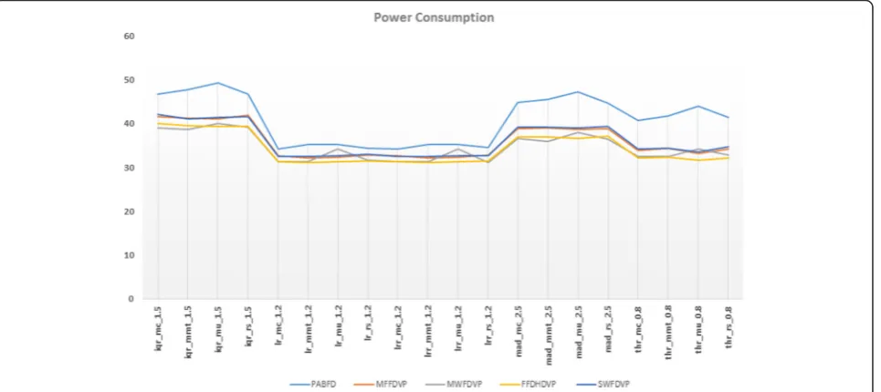
The result for power consumption produced by our pro-posed algorithms is given in Fig. 1. From that figure we can see that for any chosen policy, CloudSim’s default PABFD resulted in higher power consumption followed by almost close results of SWFDVP and MFFDVP, then MWFDVP and the last is FFDHDVP. Therefore, all of our proposed VMplacement algorithms performed better than PABFD which is used as the default VM placement algo-rithm in CloudSim. The minimum power consumption is scored by both lrmmt 1.2 and lrrmmt 1.2 as a result of selecting FFDHDVP algorithm, which draw very good re-sult compared to PABFD. Here the lrmmt means we use LR overload detection method and MMT as VM selection method where the threshold for LR is 1.2.
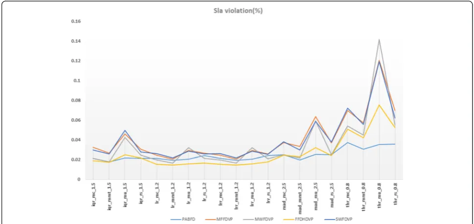
Now let us consider to the result of SLA violation which is given in Fig. 2. We could see that almost for all policies, MWFDVP, MFFDVP and SWFDVP resulted in higher SLA violation. PABFD and FFDHDVP managed
to produce lower amount of SLA violation but for thrrc 0.8, thrmmt 0.8, thrmu 0.8 and thrrs 0.8, PABFD per-formed better results compared to others. Though PABFD was overall good performer, the lowest amount of SLA was scored by lrmmt 1.2 and lrrmmt 1.2 which used FFDHDVP as VM placement algorithm. So for lowest amount of SLA violation, again our proposed FFDHDVP produced better results compared to Cloud-sims default PABFD algorithm.
In Fig. 3, we have shown the performance degradation due to VM migration for all of our proposed VM place-ment algorithms against PABFD. We can see from the figure that throughout the policies while using lrmmt 1.2 and lrrmmt 1.2, MWFDVP algorithm caused smal-lest amount of performance degradation, followed by FFDHDVP (the difference between them was 0.01 % which is very small), MFFDVP, SWFDVP and PABFD respectively.
Fig. 2SLA Violation (%) for non-clustered approach
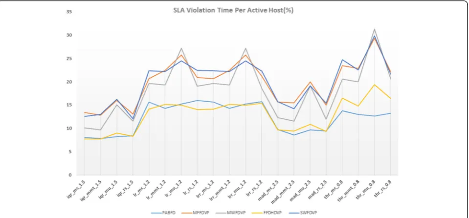
Now we will discuss about the result of SLA violation time per active host generated by all the policies that include all our proposed algorithms and CloudSim’s by de-fault PABFD algorithm. The result is given in Fig. 4. We can see from the figure that in 7.77 % of time active hosts experienced 100 % of CPU utilization while using iqrmc 1.5 policy and FFDHDVP algorithm. For VM placement both FFDHDVP and PABFD prodcuced good results but FFDHDVP got a slight edge over PABFD for causing smal-lest amount of SLA violation time per active host.
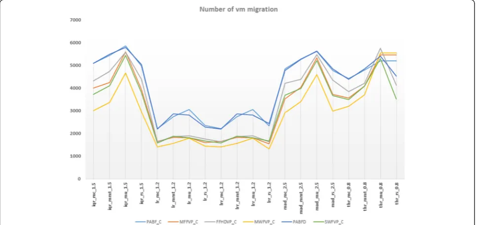
Now at last, we will examine the result of number of VM migrations for all VM placement algorithms. The result is given in Fig. 5, and we can see that lrmc 1.2 and lrrmc 1.2 scored minimum number of VM migration, when it is used with MWFDVP algorithm. After MWFDVP, MFFDVP scored second followed by FFDHDVP, SWFDVP and PABFD respectively.
In summary we can say that for power consumption, SLA violation and performance degradation due to host migration, both lrmmt 1.2 and the robust version of lrmmt which is lrrmmt 1.2 made very good results, compared with rest of the policies; for SLA violation time per active host iqrmc 1.5 and for number of VM migration both lrmc 1.2 and lrrmc 1.2 produced good results. If we want to find the best policy among all considering the metrics lrmmt 1.2 and lrrmmt 1.2 gave us quite satisfactory results. For VM placement, in every case all our proposed algorithm produced good result compared to the PABFD algorithm that is the default VM placement technique in CloudSim toolkit.
E. Result and analysis for clustering approach:
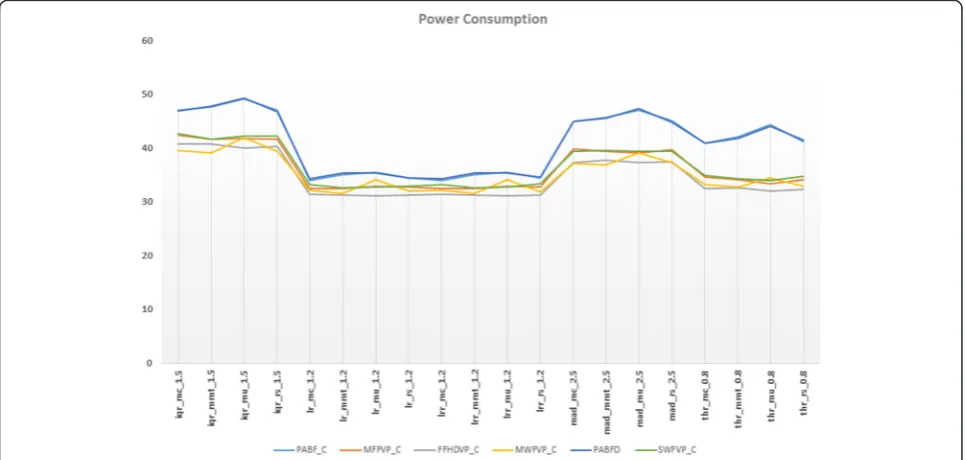
After running simulations we can see from Fig. 6 that, for any chosen policy for VM placement, original PABFD with our clustered method that used PABFD (PABF_C) resulted in higher power consumption followed by almost close results of SWFVP_C and MFFVP_C, then MWFVP_C and last FFHDVP_C, so all of our proposed VM placement algorithms with clustering, performed better than PABFD which was enabled by default in CloudSim. The minimum power consumption is scored by both lrmmt 1.2 and lrrmmt 1.2 as a result of selecting FFHDVP_C algorithm, which produced very satisfactory results compared to PABFD and our other proposed algorithms in terms of power consumption.
Now if we move over to the result of SLA violation which is given in Fig. 7, we could see that, for all policies MWFVP_C, MFFVP_C and SWFVP_C resulted in higher SLA violation. PABF_C followed by FFHDVP_C managed to produce lower amount of SLA violation for thrrc 0.8, thrmmt 0.8, thrmu 0.8 and thrrs 0.8, PABF_C showed good results compared to others. Though PABF_C was overall good performer, the lowest amount of SLA was scored by lrmmt 1.2 and lrrmmt 1.2 which used FFHDVP_C. So for lowest amount of SLA viola-tion, again our proposed FFHDVP_C produced
satisfac-tory results compared to CloudSim’s by default PABFD
and our other proposed algorithm.
Now, in Fig. 8, we have showed the output generated of performance degradation due to VM migration for all the policies of all our proposed algorithms. We can see from the picture that throughout the policies again lrmmt 1.2 and lrrmmt 1.2 caused smallest amount of performance degradation, this time MWFVP_C algorithm was the best
performer followed by FFHDVP_C, MFFVP_C, SWFVP_C and last PABF_C.
Now we will discuss about the result of SLA violation time per active host, generated by all the policies which followed all our proposed algorithms and CloudSim’s by default PABFD algorithm. The result is given in Fig. 9 and what we can see from the picture is that for 7.38 % of time, active hosts experienced 100 % of CPU utilization using iqrmmt 1.5 as overload detection policy and
FFHDVP_C algorithm as their VM placement algorithm. Both FFHDVP_C and PABF_C gave good results but FFHDVP_C got a slight edge over PABF_C for causing smallest amount of SLA violation time per active host.
Now at last, we will examine the result of number of VM migrations for all the policies that followed all the VM placement algorithms. The result is given in Fig. 10, and we can see lrrrs 1.2 scored minimum number of VM migration, when it used MWFVP_C algorithm for
Fig. 5Number of VM Migration for non-clustered approach
VM placement. For VM placement after MWFVP_C; MFFVP_C followed by FFHDVP_C, SWFVP_C and PABF_C scored good result.
Therefore, at the end of running all simulation, if we try to figure out which policy produced satisfactory results for a randomly chosen day, we can see that for power consumption, SLA violation and performance degradation due to host migration, both lrmmt 1.2 and lrrmmt 1.2 made very good results, compared with rest of the policies; for SLA violation time per active host
iqrmmt 1.5 and for number of VM migration lrrrs 1.2 pro-duced good results. If we consider to find the best policy considering all of them, we can see that being lagging be-hind in some of the cases (which is very negligible) lrmmt 1.2 and lrrmmt 1.2 gave us quite satisfactory results. For VM placement, in every cases all our proposed algorithms produced better result compared to the PABFD algorithm that was default VM placement techniquein CloudSim toolkit. However, among these algorithms, for power con-sumption, SLA violation and SLA violation time per active
Fig. 7SLA violation (%) in clustered approach
host FFHDVP_C, for performance degradation due to mi-gration and number of VM mimi-gration MWFVP_C (having close contest with FFHDVP_C) showed strong results compared to other.
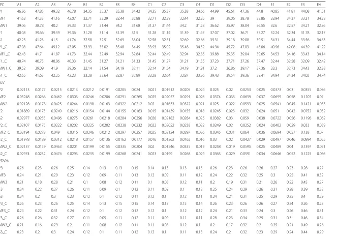
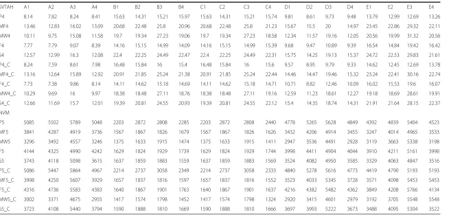
We have included the data table, i.e., Table 1 from which the graphs (Figs. 1, 2, 3, 4, 5, 6, 7, 8, 9, 10) were drawn at the very end of this paper. For fitting the data table we have shortened the name of the policies and the VM placement algorithms in the given data table.
Policies like iqr_mc_1.5, iqr_mmt_1.5, iqr_mu_1.5,
iqr_rs_1.5, lr_mc_1.2, lr_mmt_1.2, lr_mu_1.2, lr_rs_1.2,
lrr_mc_1.2, lrr_mmt_1.2, lrr_mu_1.2, lrr_rs_1.2,
mad_mc_2.5, mad_mmt_2.5, mad_mu_2.5, mad_rs_2.5, thr_mc_0.8, thr_mmt_0.8, thr_mu_0.8 and thr_rs_0.8 have been represented by A1, A2, A3, A4, B1, B2, B3, B4, C1, C2, C3, C4, D1, D2, D3, D4, E1, E2, E3 and E4 respectively.
VM placement algorithms like PABFD, MFFDVP, MWFDVP, FFDHDVP, and SWFDVP have been repre-sented by P, MF, MW, F and S respectively for
non-Fig. 9SLA Violation Time per Active Host (%) in clustered approach
MF1 41.63 41.33 41.16 42.07 32.71 32.29 32.44 32.88 32.71 32.29 32.44 32.85 39 39.06 38.78 38.86 33.94 34.37 33.31 34.28
MW1 39.06 38.78 40.2 39.33 31.37 31.44 34.2 31.68 31.37 31.44 34.2 31.23 36.62 35.97 38.04 36.55 32.6 32.57 34.21 32.86
F1 40.08 39.66 39.39 39.36 31.28 31.14 31.39 31.5 31.28 31.14 31.39 31.47 37.07 37.02 36.71 37.27 32.24 32.34 31.78 32.17
S1 42.23 41.23 41.5 41.74 32.58 32.51 32.69 33.04 32.58 32.51 32.69 32.66 39.31 39.18 39.08 39.51 34.31 34.44 33.56 34.83
P1_C 47.08 47.64 49.12 47.05 33.93 35.02 35.48 34.49 33.93 35.02 35.48 34.52 44.94 45.72 47.03 45.06 40.96 42.08 44.39 41.22
MF1_C 42.43 41.7 41.87 41.73 32.44 32.49 32.94 32.84 32.44 32.49 32.94 32.85 39.88 39.35 39.04 39.65 34.53 34.16 33.43 34.14
F1_C 40.74 40.75 40.06 40.33 31.45 31.27 31.21 31.33 31.45 31.27 31.21 31.35 37.23 37.71 37.26 37.47 32.44 32.58 32.09 32.42
MW1_C 39.52 39.09 41.9 39.36 32.14 31.54 34.19 32.11 32.14 31.54 34.19 31.91 37.2 36.86 39.17 37.36 33.3 32.73 34.43 32.88
S1_C 42.65 41.63 42.25 42.23 33.28 32.64 32.87 32.89 33.28 32.64 32.87 33.36 39.43 39.54 39.36 39.41 34.94 34.34 34.02 34.74
SLV
P2 0.02113 0.0177 0.0215 0.0213 0.0212 0.0191 0.0205 0.024 0.021 0.01912 0.0205 0.024 0.025 0.02 0.0253 0.025 0.0373 0.03 0.0355 0.036
MF2 0.03248 0.0266 0.0462 0.0303 0.0246 0.0206 0.0291 0.0265 0.025 0.02057 0.0291 0.026 0.0374 0.033 0.0639 0.037 0.0699 0.058 0.1207 0.07
MW2 0.02128 0.0178 0.0425 0.0244 0.0198 0.0163 0.0322 0.0212 0.02 0.01633 0.0322 0.021 0.025 0.022 0.0593 0.025 0.0541 0.045 0.1421 0.055
F2 0.01889 0.0175 0.0249 0.0216 0.0154 0.0144 0.0155 0.0163 0.015 0.01439 0.0155 0.018 0.0245 0.023 0.032 0.024 0.051 0.042 0.0752 0.052
S2 0.02977 0.0255 0.0496 0.0275 0.0261 0.0218 0.0284 0.0256 0.026 0.02182 0.0284 0.025 0.0382 0.03 0.059 0.038 0.0722 0.056 0.1196 0.062
P2_C 0.02107 0.0175 0.0222 0.0202 0.0225 0.0202 0.0238 0.0232 0.022 0.02022 0.0238 0.022 0.0249 0.02 0.0252 0.024 0.0402 0.029 0.033 0.039
MF2_C 0.03194 0.0278 0.049 0.0316 0.0246 0.0212 0.0297 0.0257 0.025 0.02124 0.0297 0.026 0.0345 0.031 0.064 0.036 0.0694 0.057 0.138 0.07
F2_C 0.01978 0.0189 0.0312 0.0218 0.0157 0.0136 0.0162 0.0177 0.016 0.01362 0.0162 0.016 0.03 0.02 0.0427 0.029 0.0497 0.046 0.0894 0.055
MW2_C 0.02137 0.0159 0.0463 0.0201 0.0199 0.0155 0.0335 0.0204 0.02 0.01546 0.0335 0.019 0.0258 0.019 0.0595 0.025 0.0489 0.04 0.1397 0.051
S2_C 0.02974 0.0232 0.0474 0.0293 0.0235 0.0199 0.0268 0.0241 0.023 0.0199 0.0268 0.029 0.0363 0.029 0.0591 0.034 0.0646 0.052 0.1225 0.066
PDVM
P3 0.26 0.23 0.26 0.25 0.14 0.13 0.13 0.15 0.14 0.13 0.13 0.15 0.26 0.23 0.26 0.26 0.27 0.23 0.28 0.27
MF3 0.24 0.21 0.29 0.23 0.12 0.09 0.11 0.13 0.12 0.09 0.11 0.12 0.24 0.22 0.32 0.25 0.3 0.25 0.41 0.32
MW3 0.21 0.18 0.28 0.21 0.1 0.08 0.12 0.11 0.1 0.08 0.12 0.11 0.2 0.19 0.31 0.21 0.26 0.22 0.45 0.27
F3 0.24 0.22 0.27 0.26 0.11 0.09 0.1 0.12 0.11 0.09 0.1 0.12 0.25 0.24 0.29 0.26 0.31 0.28 0.39 0.32
S3 0.24 0.2 0.3 0.23 0.12 0.1 0.12 0.11 0.12 0.1 0.12 0.11 0.24 0.21 0.31 0.25 0.29 0.25 0.4 0.29
P3_C 0.26 0.23 0.26 0.25 0.14 0.13 0.15 0.15 0.14 0.13 0.15 0.14 0.26 0.23 0.26 0.26 0.27 0.24 0.26 0.28
MF3_C 0.24 0.22 0.31 0.24 0.12 0.1 0.12 0.12 0.12 0.1 0.12 0.12 0.24 0.21 0.33 0.24 0.3 0.26 0.46 0.31
F3_C 0.26 0.26 0.32 0.27 0.11 0.09 0.11 0.12 0.11 0.09 0.11 0.11 0.28 0.23 0.34 0.29 0.31 0.3 0.46 0.34
MW3_C 0.21 0.16 0.29 0.2 0.11 0.08 0.12 0.11 0.11 0.08 0.12 0.1 0.2 0.17 0.32 0.2 0.25 0.21 0.49 0.26
S3_C 0.23 0.2 0.3 0.24 0.12 0.1 0.11 0.12 0.12 0.1 0.11 0.13 0.24 0.2 0.32 0.23 0.29 0.24 0.44 0.29
et
al.
Journal
of
Cloud
Computing:
Advances,
Systems
and
Applicati
ons
(2015) 4:20
Page
15
of
MF4 13.46 12.83 16.02 13.09 20.68 22.48 25.8 20.96 20.68 22.48 25.8 21.23 15.67 15.5 20 14.97 23.45 22.86 29.32 22.11
MW4 10.11 9.75 15.08 11.58 19.7 19.34 27.23 19.06 19.7 19.34 27.23 18.58 12.34 11.57 19.16 12.05 20.56 19.99 31.32 20.56
F4 7.77 7.79 9.07 8.39 14.16 15.15 14.99 14.09 14.16 15.15 14.99 15.39 9.68 9.47 10.89 9.39 16.54 14.84 19.42 16.42
S4 12.57 12.99 16.3 12.08 22.4 22.25 24.49 22.47 22.4 22.25 24.49 22.31 15.75 14.25 19.13 15.37 24.72 22.53 29.83 21.61
P4_C 8.24 7.59 8.61 7.98 16.48 15.84 16 15.4 16.48 15.84 16 15.6 9.57 8.95 9.79 9.33 14.62 12.45 12.69 13.78
MF4_C 13.16 12.64 15.89 12.92 20.91 21.85 25.24 21.38 20.91 21.85 25.24 22.44 14.46 14.47 19.46 15.32 23.24 22.41 30.16 22.74
F4_C 7.73 7.38 9.86 8.14 14.11 14.62 15.18 14.69 14.11 14.62 15.18 14.71 10.71 8.82 12.46 10.09 16.02 15.53 19.6 16.07
MW4_C 10.29 9.69 16 9.97 18.38 18.48 27.11 18.76 18.38 18.48 27.11 19.16 12.59 11.23 18.61 12.27 19.18 18.69 28.61 19.91
S4_C 12.66 11.69 15.7 12.01 19.39 20.81 24.55 20.93 19.39 20.81 24.55 22.12 15.4 14.35 18.74 14.31 21.91 21.64 28.15 22.37
NVM
P5 5085 5502 5789 5048 2203 2872 2808 2285 2203 2872 2808 2440 4778 5265 5628 4849 4392 4839 5404 4523
MF5 3841 4287 4919 3736 1567 1867 1826 1679 1567 1867 1826 1626 3432 4206 4914 3455 3247 4014 4965 3533
MW5 3296 3492 4557 3246 1375 1633 1915 1474 1375 1633 1915 1411 2947 3536 4491 2928 3119 3663 5338 3198
F5 4144 4325 4990 4242 1629 1824 1929 1739 1629 1824 1929 1744 3998 4411 4904 4044 3910 4211 5161 3998
S5 3743 4118 5098 3615 1637 1859 1883 1559 1637 1859 1883 1569 3524 4082 4950 3585 3329 4063 4847 3516
P5_C 5086 5447 5864 4967 2214 2737 3058 2349 2214 2737 3058 2333 4840 5278 5616 4773 4419 4790 5193 5193
MF5_C 3998 4250 5607 3929 1657 1837 1816 1597 1657 1837 1816 1552 3523 4033 5345 3728 3571 4098 5453 5453
F5_C 4316 4736 5583 4383 1640 1867 1901 1763 1640 1867 1901 1637 4216 4382 5482 4362 3849 4208 5766 4134
MW5_C 3002 3371 4675 2955 1417 1574 1798 1452 1417 1574 1798 1324 2920 3415 4601 2979 3192 3705 5548 5548
S5_C 3723 4108 5440 3794 1590 1888 1810 1669 1590 1888 1810 1666 3697 3993 5222 3673 3488 4095 5304 3522
et
al.
Journal
of
Cloud
Computing:
Advances,
Systems
and
Applicati
ons
(2015) 4:20
Page
16
of
clustering approach. As we have taken into account five matrices, in order to differentiate those matrices in the data table, we represented them as numeric numbers, such as power consumption has been represented by PC and SLA violation, performance degradation due to VM migration, SLA violation time per active host, number of VM migration have been represented by SLV,PDVM, SVTAH,NVM respectively. For example P1 means power consumption while using PABFD algorithm and P5 means number of VM migration while using PABFD algorithm. We followed the same naming convention for clustering approach, so for example P1_C means power consumption while using PABF_C algorithm and P5_C means number of VM migration while using PABF_C algorithm.
F. Comparison among clustering and non-clustering approach
In the previous section, we individually showed results of our VM placement algorithms for both non-clustered
and clustered approach with different VM selection and overload detection policies. On both cases we ran our simulation for one day data from ten days PlanetLab workload traces. We have seen that our proposed VM placement algorithms did very well compared to the PABFD algorithm in all perspectives, i.e., all performance metrics.
To extend our study and analyze the algorithms further, we use other statistical measures which quanti-tatively describe the measurements from our results. We want to find the degree of spread as well as mea-sures of skewness of the performance for clustered and non-clustered approaches. To graphically depict the comparison, we use box plot that records minimum. maximum, average, and different percentile values of the metrics. The box plot also demonstrates the spread and deviation in performance. For this, we use all ten days data. The day wise PlanetLab data is given in Table 2. These data could be accessed from github re-pository of Beloglazov [https://github.com/beloglazov/ planetlab-workload-traces].
However, if we consider every VM placement, VM selec-tion and overload detecselec-tion techniques, the number of combinations is huge, i.e., 10 VM placement strategies (5 clustered and 5 non-clustered), 3 VM selection strategies and 5 overload detection strategies. If we want to consider all of them, 150 comparisons should be made which is huge and considerable amount of simulation time is required to report the findings. As we already found our best two VM Placement techniques as FFDHDVP and MWFDV, we consider them for further analysis. So, we took only FFDHDVP and MWFDVP for non-clustered, FFHDVP_C and MWFVP_C for Clustered VM placement algorithms and selected policies like lrrmmt 1.2, lrrmc 1.2, and iqrmc1.5. We skipped policies like lrmmt 1.2 and lrmc1.2 as they scored exactly the same as their robust versions. Table 2Day wise planet lab data
Data Number of VMs
3 March 1052
6 March 898
9 March 1061
22 March 1516
25 March 1078
3 April 1463
9 April 1358
11 April 1233
12 April 1054
20 April 1033
The result of this descriptive statistic is discussed below. In the figures we used numbers to reflect policies name so that they can visibly fit into our graphs. We used #1, #2, and #3 to represent iqrmc 1.5, lrrmmt 1.2 and lrrmc 1.2 respectively. For example PABFD#1 means we used PABFD as our VM placement algorithm and iqrmc 1.5 as our VM selection and overload detection policy, i.e., iqr as overload detection with threshold 1.5, mc as maximum correlation VM selection policy.
By comparing our proposed VM placement algorithms against existing algorithm like PABFD it is found from Fig. 11 that, the power consumption is remarkably reduced in proposed FFDHDVP algorithm. Minimum energy consumption is 86.09 Kwh for lrrmmt 1.2 where the minimum of PABFD is 122.88 Kwh for the same pol-icy; therefore we got 29.93 % reduction. Considering average values, FFDHDVP consumed 112.646 Kwh and PABFD consumed 161.87 Kwh on average for lrrmmt 1.2, resulting 24 % of energy saving.
From Fig. 12, we can see that SLA violation is signifi-cantly decreased when we used FFHDVP_C as VM place-ment algorithm and lrrmmt 1.2 as our policy. FFHDVP_C resulted 0.00087 %SLA violation in minimum compared to PABFD’s 0.00439 % which indicates 80 % reduction. If we consider average value, FFHDVP_C produced 0.001447 % SLA and PABFD incurred 0.004974 % on average, resulting 71 % reduction in SLA violation.
For performance degradation due to VM migration what we can see from Fig. 13, is that for lrrmmt1.2, MWFVP_C scored minimum PDM of 0.033296 % and PABFD scored 0.0734734 % resulting 54.68 % of
im-provement. If we count the average value MWFVP_C’s
0.041294 % PDM beat PABFD’s 0.07969383 % PDM by
reduction of 48 %.
Figure 14 describes the result of SLA violation time per active host. We can see from the figure FFHDVP_C scored minimum SLATAH of 2.53 % for lrrmmt1.2 and PABFD scored 5.84 %, causing 56 % improvement.
Fig. 12SLA violation (%) for clustered, non-clustered and default methods
Counting average values we can see that both FFHDVP_C and PABFD caused 3.349 % and 6.213 % SLATAH for lrrmmt 1.2, resulting 46 % improvement over SLATAH.
Now at last we will move on to the results of number of VM migration. The result is given in Fig. 15 and we can see from the output that the minimum amount of
VM migration for FFHDVP_C is 8449 and PABFD’s
minimum is 16903 for lrrmc 1.5 policy, indicating 50 %
less migration of VM. For average, FFHDVP_C’s 11890
VM migration outperformed PABFD’s 23931 VM
migra-tion causing 50 % improvements.
We could say that when lrrmmt 1.2 is chosen as VM selection and overload detection policy, for reducing power consumption FFDHDVP, for SLA violation, SLA violation time per active host and number of VM migra-tion our clustered FFHDVP_C and, for performance degradation due to migration clustered MWFVP_C
made outstanding results. So, we can say that all of our proposed algorithms outperformed PABFD algorithm that was the default VM placement algorithm given in CloudSim toolkit.
Finally, we have performed a statistical test namely two-tailed students’t-test on the performance of PABFD and the best VM placement algorithm, i.e., FFHDVP_C, in this research. Our null hypothesis is: “There is no significant difference in the performance between two techniques”. Table 3 reports p-values for five performance metric be-tween PABFD and FFHDVP_C generated from ten days experimental data.
If the p-value is greater than 0.05, then we must accept the null hypothesis, otherwise we must reject the null hypothesis. From Table 3 we find that the p-value is sig-nificantly smaller than 0.05 for every performance metric. Therefore, we must reject the null hypothesis and we could conclude that there is significantly
Fig. 14SLA violation time per active host for clustered, non-clustered and default methods
difference in performance found by the built in Power Aware Best Fit Decreasing (PABFD) in CloudSim and the best algorithm, FFHDVP_C that we develop and im-plement in this research. From the box plots, we could easily verify that our proposed algorithms perform sig-nificantly better than the built in PABFD VM placement algorithm
Conclusion
Using different solutions of bin packing problem, our pro-posed VM placement algorithm could make remarkable improvements over the existing solution. Our proposed techniques managed to get lower power consumption, less amount of SLA violation and less amount of performance degradation over the existing PABFD VM placement algo-rithm. We are also successful to show that VM placement is favored by higher virtual machine density which we proved by adopting clustering method. From our result we also find out that local regression based algorithm equipped with the minimum migration time VM selection policy significantly outperforms other dynamic VM con-solidation algorithms. As a future work we plan to intro-duce fuzzy algorithm that could take advantages from different selection criteria and form a rule base for VM se-lection. We also suggest for making more ecofriendly IT infrastructures with reasonable amount of on-demand op-erating cost to improve the quality of IaaS of cloud computing.
Competing interests
The authors declare that they have no competing interests.
Authors’contributions
In the paper, we have implemented multiple redesigned VM placement algorithms and introduced a technique by clustering VMs to migrate by taking account both CPU utilization and allocated RAM. We implement and study the performance of our algorithms on Cloud computing simulation toolkit known as CloudSim using PlatenLab workload data. Simulation results demonstrate that our proposed approach outperforms the default VM Placement algorithm designed in CloudSim. All authors read and approved the final manuscript.
Acknowledgement
There is no acknowledgement from authors’side.
Received: 30 May 2015 Accepted: 29 October 2015
References
1. Fan X, Weber WD, Barroso LA (2007) Power provisioning for a warehouse-sized computer. Proceedings of the 34th Annual International Symposium on Computer Architecture (ISCA 2007), ACM New York, NY, USA, pp 13–23 2. Hyukho K, Woongsup K, Yangwoo K (2010) Experimental study to improve
resource utilization and performance of cloud systems based on grid middleware. J Commun Comput 7(12):32–43
3. Beloglazov A, Buyya R (2012) Optimal online deterministic algorithms and adaptive heuristics for energy and performance efficient dynamic consolidation of virtual machines in Cloud data centers. Concurrency Computat. Pract Exper 24:1397–1420. doi:10.1002/cpe.1867 4. Ajiro Y, Tanaka A (2007)“Improving packing algorithms for server
consolidation”, in Proceedings of the International Conference for the Computer Measurement Group (CMG)
5. Robert B, Hermann De M, Ricardo L, Giovanni G (2012) Cloud computing and its interest in saving energy: the use case of a private cloud”. J Cloud Comput Adv Syst Appl 1:5
6. Mohamad G, Francis G, Dagenais MR (2014) Fine-grained preemption analysis for latency investigation across virtual machines”. J Cloud Comput Adv Syst Appl 3:23
7. Ziqian D, Ning L, Roberto R-C (2015) Greedy scheduling of tasks with time constraints for energy-efficient cloud-computing data centers”. J Cloud Comput Adv Syst Appl 4:5
8. Panigrahy R, Talwar K, Uyeda L, Wider U (2011) Heuristics for Vector Bin Packing”, Microsoft’s VMM Product Group, Microsoft Research Sillicon Valley 9. Kangkang L, Huanyang Z, Jie W (2013)“Migration-based virtual machine
placement in cloud systems,”Cloud Networking (CloudNet), 2013 IEEE 2nd International Conference., pp 83–90. doi:10.1109/CloudNet.2013.6710561, 11-13 Nov
10. Khanna G, Beaty K, Kar G, Kochut A (2006) Application performance management in virtualized server environments. In: Proceedings of the 10th IEEE/IFIP Network Operations and Management Symposium, NOMS’06
11. Jung G, Joshi KR, Hiltunen MA, Schlichting RD, Pu C (2008) Generating adaptation policies for multi-tier applications in consolidated server environments. Proceedings of the 5th IEEE International Conference on Autonomic Computing (ICAC 2008), Chicago, IL, USA, pp 23–32 12. Jung G, Joshi KR, Hiltunen MA, Schlichting RD, Pu C (2009) A cost-sensitive
adaptation engine for server consolidation of multitier applications. Proceedings of the 10th ACM/IFIP/USENIX International Conference on Middleware (Middleware 2009), Urbana Champaign, IL, USA, pp 1–20 13. Bichler M, Setzer T, Speitkamp B (2006) Capacity planning for virtualized
servers, in: Proceedings of the 16th Annual Workshop on Information Technologies and Systems, WITS’06
14. Speitkamp B, Bichler M (2010) A mathematical programming approach for server consolidation problems in virtualized data centers, IEEE Transactions on Services Computing
15. Ferreto TC, Netto MAS, Calheiros RN, De Rose CAF (2011) Server consolidation with migration control for virtualized data centers. Future Gener Comput Syst 27(8):1027–1034, October 2011
16. Beloglazov A, Abawajy J, Buyya R (2011) Energy-aware resource allocation heuristics for efficient management of data centers for cloud computing. Future Generat Comput Syst. doi:10.1016/j.future.2011.04.017
17. Verma A, Dasgupta G, Nayak TK, De P, Kothari R (2009) Server workload analysis for power minimization using consolidation. Proceedings of the 2009 USENIX Annual Technical Conference, San Diego, CA, USA, pp 28–28 18. Baker BS (1985) A new proof for the first-fit decreasing bin-packing
algorithm. J Algorithms 6(1):49–70
19. Dósa G (2007) The Tight Bound of First Fit Decreasing Bin-Packing Algorithm Is FFD(I)≤11/9OPT(I) 6/9. In: Combinatorics, Algorithms, Probabilistic and Experimental Methodologies, 2007, vol 4614. Springer, Berlin Heidelberg, pp 1–11
20. Venigella, Swathi,“Cloud storage and online bin packing”(2010) UNLV Theses/Dissertations/ Professional Papers/Capstones. Paper 894. http:// digitalscholarship.unlv.edu/thesesdissertations/894. Accessed 22 April, 2015. 21. Fan X, Weber WD, Barroso LA (2007) Power provisioning for a
warehouse-sized computer. Proceedings of the 34th Annual International Symposium on Computer Architecture (ISCA 2007), ACM New York, NY, USA, pp 13–23 22. Kusic D, Kephart JO, Hanson JE, Kandasamy N, Jiang G (2009) Power and
performance management of virtualized computing environments via lookahead control. Cluster Comput 12(1):1–15
Table 3P-value for different performance metric
Metric p-value
Power Consumption 0.004118825
SLA-Violation 6.93*10-6
Performance degradation due to migration 1.83*10-13
SLA Violation per active host 3.27*10-7
23. Ausiello G, Lucertini M, Serafini P (1984) Algorithm Design for Computer System Design. Springer, Wien, Print
24. Tan P-N, Michael S, Vipin K (2005) Introduction to Data Mining. Pearson Addison Wesley, Boston, Print
25. Baswade AM, Nalwade PS (2013) Selection of initial centroids for k-means algorithm. IJCSMC 2(7):161–164
Submit your manuscript to a
journal and benefi t from:
7Convenient online submission 7Rigorous peer review
7Immediate publication on acceptance 7Open access: articles freely available online 7High visibility within the fi eld
7Retaining the copyright to your article