BLIND SOURCE SEPARATION AND
ICA TECHNIQUES: A REVIEW
SANJEEV N. JAIN*, Research scholar,
Electronics Engineering Department, S.J.J.T. University,
Vidyanagar, Churu, Jhunjhunu Road,Chudela, District-Jhunjhunu,Rajasthan-333001(India)
DR. CHANDRASHEKHAR RAI, Computer Science,
G.G.S. Indraprastha University, Sector 16-C, Dwarka, New Delhi-110075(India)
Abstract:
Blind source separation (BSS) and independent component analysis (ICA) are by and large based on a wide class of unsupervised learning algorithms and they have potential applications in many areas from applied sciences like neuroscience to engineering. The BSS exploits the priori knowledge of nature and structure of hidden sources such as sparseness, noise, gaussinity, spatio-temporal decorrelation, statistical independence. Independent component analysis (ICA) and blind source separation (BSS) refer to the problem of recovering statistically independent signals from a linear mixture. Herewith, a review of BSS and ICA has been presented with respect to the number of methods, research procedures, models developed, technological up gradation being practiced, so that the pathways of research in the field can be obtained. The paper is divided into four sections such as, a) Introduction b) Approaches & methods c) Recent developments and d) Applications.
Keyword: BSS, ICA, sparse signals, noise sources, Genetic algorithm
1. Introduction
Blind source separation was first considered in 1982 from a simple discussion between Bernard Ans, Jeanny Hérault and Christian Jutten with Jean-Pierre Roll, a neuroscientist, about motion decoding in vertebrates. Joint motion takes place because of muscle contraction; each muscle fiber is controlled by the brain, through a moto-neuron. In addition, on each fiber, the muscle contraction is measured, and the information of the same is transmitted to the central nervous system by two varieties of sensorial endings, located in tendon, and is called primary and secondary endings. For trustworthiness reasons, results are obtained by averaging unit sensory responses coming from a huge number of fibers, related to the repetition of the same forced motion. Surprisingly, while one could imagine that each type of ending only transmits one type of information, either stretching or speed, the sensory information transmitted by endings is a mixture of stretching and speed information [Simon Haykin, (1999) and Jutten C. (1987)].
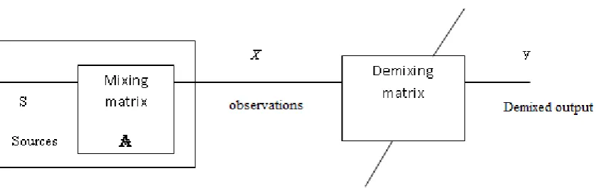
Figure 1 : Diagrammatic representation of the blind source separation technique
The perception of blind source separation is related to independent component analysis (ICA). However, ICA can be viewed as a general-purpose tool replacing principal component analysis (PCA) which means it is applicable to a wide range of problems. Some application domains of blind source separation are biomedical signal analysis, geophysical data processing, data mining, wireless communications and sensor array processing [Karhunen J. (1999)].
1.1.The BSS model :
Blind source separation (BSS) is a major area of research in signal and image processing. It aims at recuperating source signals from their mixtures without meticulous knowledge of the mixing process. The job is to calculate approximately the individual source without signals, i.e. to demix the mixture. The Blind Source Separation (BSS) problem is defined by a mixture model (see figure 2), a set of source processes, and a set of assumptions.
Figure 2 Mixing model of blind source separation
Let us denote the Nsource signals by the vector
S (t) = (S1(t), …., SN(t))T, ( 1 )
and the observed M signals are by
X(t) = (X1(t),…, XM(t))T ( 2 )
Now, the mixing can be expressed as,
X(t) = A S(t) ( 3 )
or
X(t) = A S(t) + n(t) ( 4 )
No particular assumptions on the mixing coefficients are made. However, some weak structural assumptions are often made: for example, it is typically assumed that the mixing matrix is square, that is, the number of source signals equals the number of observed signals (M = N), the mixing process Ais defined by an even-determined (i.e. square) matrix and, provided that it is non-singular, the underlying sources can be estimated by a linear transformation.
Also, n (t) = (n1 (t),… nM(t))Tis a vector of additive noise. The problem of BSS is now to guess both the source signals Sj(t )and the mixing matrix A based on observations of the Xi (t)alone. The task of BSS is to recuperate the original signals from the observations X(t) without the knowledge of A nor S(t). There are a number of factors that are expected to affect the separation performance in applications, such as the number of active sources, the distribution of source signals, time-variable mixtures, and noise.
The strength of this model is that the two independence assumptions stated above are physically possible in several instances and are strong enough to offer some kind of identifiability. In a blind context, the separation of sources can only rely on the basic knowledge of their mutual independence.
A classical example of blind source separation is the cocktail party problem. Assume that several people are speaking concurrently in the same room, as in a cocktail party. Then the problem is to separate the voices of the different speakers, using recordings of several microphones in the room. Cocktail party problem is a standard scientific problem that has been studied for years. Humans have remarkable skills in separating target speech from a complex auditory mixture obtained in a cocktail party environment. Computational modeling for such a mechanism is however tremendously challenging [Amari S.and Cichocki A. (1998 ),
Amari S., et al.(1996) ]. In order for human to ‘pick out’ a voice from a group of voices in a crowded room, one must perform some type of BSS to recuperate the original sources from the observed mixture. Mathematically, it’s necessary to find a demixing matrix W, which when multiplied by the recordingsXT, produces an estimate yT of the sources ST. Therefore W is a set of weights (approximately 16) equal to A−1.
The BSS issue can be divided into three categories depending upon the number of sources & the number of sensors used to detect the same.
1. Number of sources (S1,S2) < number of sensors (X1,X2,X3) :Overdetermined mixing
2. Number of sources (S1,S2) = number of sensors (X1,X2) :Determined mixing
3. Number of sources(S1,S2,S3) > number of sensors (X1,X2) :Underdetermined mixing
In BSS; the goal is to extract independent source signals from their linear mixtures using minimum of priori of information or the goal of BSS is to reconstruct the sources from the observations. Clearly, for this task to be possible A should not be entirely unknown: it should belong to some class of transformations given A a
overload.” The problem is to access large amounts of data containing relatively small amounts of useful information. This is true both in daily lives, and within many scientific disciplines [Comon P. (1992 a), (1994 b)].
Independence is associated to probability and statistics, and tools borrowed from these fields bring a lot to source separation. For instance, the factorial analysis, intensively studied in statistics in the 1950s, is another way to formalize ICA, especially the separability problem.
Independent component analysis (ICA) and blind source separation (BSS) refer to the problem of recovering statistically independent signals from a linear mixture. There is variety of situations where signals are originated as combination of independent processes or sources. Here are just a few examples:
1. Cocktail-Party-Problem: Sound amplitudes in a acoustic environment add up linearly. Multiple sound sources such as speakers, music or noise sources are measured by the microphones as a mixture. The question is, how can one recover the individual speakers?
2. Hyper-spectral sub-pixel identification: Hyper-spectral imagery consists of a set of images taken at
different wavelengths - currently up to 200. Every material on the surface, i.e. rock, grass, trees, snow, etc. have different reflection coefficients at every wavelength. The area corresponding to a pixel contains usually a mixture of different surface materials, as the resolution is still in the range of a few square meters. The intensities in every pixel are therefore a linear combination of the abundances of materials and the reflection coefficients of each material. The problem is then, how to identify the surface materials and their abundance?
3. Passive sonar: In passive sonar a large number of sensors (microphones) records signals originating
from multiple sources such as shrimp noise, submarines engines, boats, etc. Every sensor records a different mixture as they are places in different locations and the amplitudes vary with distance from the sources. The task is to separate and identify the sound sources.
In BSS, for instance, various types of mixture can be considered, as: (i) instantaneous (i.e. static) linear mixtures, (ii) convolutive mixtures, or (iii) nonlinear mixtures. Convolutive blind source separation (CBSS) refers to the separation of signals that have been mixed through a dispersive environment using signal processing procedures that do not have specific knowledge of the source properties or the mixing conditions. The aim of the convolutive BSS is to find filters that when applied to X(ݐ) result in new signals ݕ(ݐ), which is a model of the original source signals S(ݐ).
The mixing operation is often assumed to be invertible, but it is not the case for under-determined mixtures. Source signals can take their values in the real field or in the complex field, be of constant modulus or belong to a finite alphabet, a priori known or not. When source signals are considered to be random, several assumptions exist. Sources may be:
(a) Mutually statistically independent,
(b) Each identically and independently distributed in time (IID), or
(c) Cyclo-stationary.
Mixture models considered remain deterministic, and depend on some constant unknown parameters. Once this class of parametric models is fixed, the Blind Identification problem will consist of estimating these parameters only from the observation of the outputs of the system.
In all cases, the question will always be the following. Given a mixture model and a set of assumptions:
1. Can the mixture be identified from the observations?
2. Can the source signals be separated, i.e. consistently estimated?
3. What algorithm can be used to perform these tasks?
Contrast functions put forth the answer of first two questions. In fact, a contrast function can be defined as an optimization criterion such that all its global maxima correspond to a separation of all sources. Defining a contrast criterion leads to the property of source separability. Once the optimization criterion is defined, it remains to devise a numerical algorithm to maximize it [Olyaee S., et al (2010)].
In the years following the publication of the early works, the theory and practice of blind source separation have been studied rigorously. Many different algorithms have been proposed for BSS. These algorithms have proven practical in varied areas of application.
2. Approaches & Methods adopted:
The different approaches started developing from 1994. Since then, Comon, Bell and Sejnowski have three contributions. First, neural network with sigmoid nonlinear function was employed to cancel the high-order statistic correlation in the measured signals. Second, the study established contrast function on the principle of information maximization, thereby integrating ICA and information theories. Third, it developed a line iteration learning algorithm (Infomax algorithm), which successfully separated ten mixed voice signals. However, the algorithm requires matrix inverse and the convergence speed is slow. The effectiveness of the algorithm is affected by the ways of mixture in the original signals. It can only separate super Gaussian signals. In 1999, Hyvärinen proposed a fast iteration algorithm called FastICA, with greatly increased convergence speed. The major applications of ICA may be divided into two types, one is InfomaxICA proposed by Lee in 1998 and the other is FastICA by Hyvärinen in 1999. The latter is based on artificial neural network learning algorithm [Lin S.and Tung P.(2006)].
2.1.Frequency & time domain:
The existing algorithms for solving BSS problem can be mainly divided into two different categories: the algorithms in the time domain and the algorithms in the frequency domain. Comparison within these algorithms; the time domain algorithm result in better performance, because of frequency domain algorithms have to take into account a permutation and scaling ambiguity at each frequency, furthermore, to provide good results, these methods may require a large number of samples. Also the frequency domain approach exploits a large number of frequency bins, therefore increase the computation cost. The advantage of the time domain approaches has been summarized as: the better independence assumption for full-band signals and possible high convergence near the optimal point. The disadvantages mentioned of these approaches are degradation of convergence in strong reverberant environment and need many parameters to be adjusted for each iteration step. So based on these inferences out of the time domain & frequency domain approaches of BSS it has been proved [Olyaee S., et al (2010)] that the time domain algorithm is theoretically consistent without any permutation and amplitude indeterminacy problems. Further, the limitation of the frequency domain algorithm is studied [Araki S et al.(2001)] while analyzing the separation of real acoustic signal. The main difficulties reported in [Kamran R. and Reilly J. (2002)] with frequency domain blind source separation of convolutive mixtures is the arbitrary permutation and scaling ambiguities of the estimated frequency response of the un-mixing system at each frequency bin.
whitening matrix W can be determined from the covariance matrix & then the second step determines the unitary matrix u. The mixing matrix A
is easily computed, since u = W
A
, and so are the sources, since X(t) = A S (t). SOBI is suggested as an interesting alternative to ICA for sources with different spectral contents, which is often the case in structural dynamics.
Structure from motion (SfM) is a common approach reported & further studied by Fortuna J. and Martinez A. (2006) to recover the 3D shape of an object observed over multiple frames of an image sequence. With no information available about the joint density of three-dimensional points, the assumption of independence is the only reasonable one.
2.2.Genetic Algorithm:
The genetic algorithm (GA) based BSS methods have been developed by Gorriz J., et al (2006) and Tan Y. , Wang J. (2001)] and which are characterized by high accuracy, high robustness, and fast convergence with the moderate assumptions as 1) the parametric form of mixtures is known; 2) signal sources are statistically independent; and 3) the number of sensors is equal to that of sources. These studies have revealed that GA algorithm can be used in case of linear & nonlinear mixtures. It is concluded that though it performs in both the cases nonlinear mixture separation can be performed in a better manner. Convergence and separation performance are said to be [Nakayama k., et al.(2002)] highly dependent on relation between a probability density function (pdf) of signal sources and nonlinear functions used in updating parameters in a separation block. A novel algorithm is proposed and it [Zheng C., et al. (2006)] is based on minimizing mutual information for a special case of nonlinear blind source separation.
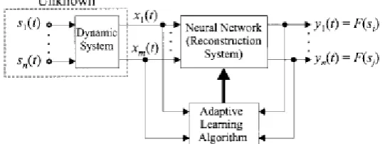
Rai C.S.and Singh Y.(2004 a), (2002 b) proposed an approach which is considered for characterizing the source distributions. Various methods have been proposed to separate mixtures of sub- and super-Gaussian signals. Effectiveness of a blind source separation algorithm depends upon the source distribution model used for deriving the weight update rule. This approach leads to appropriate handling of both kinds of signals simultaneously. Another approach presented in [Singh Y.and Rai C. S. (2003)] concludes that non linearity is best suited for sub-Gaussian signals, while extracting original independent signals with the help of observations obtained at the sensors and using the unsupervised learning algorithms for the same. A team of scientists suggested application of neural blind separation techniques in [Karhunen J., et al.(1997)] to extraction of features from natural images and to separation of medical EEG signals. Similarly, the problem of recovering communication signals (that are transmitted by unknown channels) from the received signals in the presence of both inter user and inter symbol interferences is treated with [Amari S. and Cichocki A.(1998)] the natural gradient learning algorithm instead of the ordinary gradient descent method (fig no. 3).
2.3.Underdetermined Approach:
The conventional blind source separation (BSS) algorithms are relevant when the number of sources equals to that of observations; but, they are inappropriate when the number of sources is more than that of observations. A classical study of underdetermined BSS (UBSS) has been carried out with two existing algorithms: namely the EMD (empirical mode decomposition) algorithm and a parametric estimation algorithm using ESPRIT technique. Researchers have mentioned some existing methods for the underdetermined BSS (UBSS) which include the matching pursuit methods, the separation methods for finite alphabet sources in, the probabilistic-based (using maximum a posteriori criterion) methods and the sparsity-based techniques. In [Abdeldjalil, et al. (2007)], an alternative approach named MD-UBSS (modal decomposition UBSS) using modal decomposition of the received signals is proposed. This paper introduces a new blind separation method for audio-type sources using modal decomposition. The proposed method can separate more sources than sensors and provides a better separation quality than the one obtained in the instantaneous mixture case.
The BSS is formulated with general Eq. 1, where A
is an N x N square matrix. In BSS the goal is to find an
N x N invertible square matrix W such thatu = W X ( 5 )
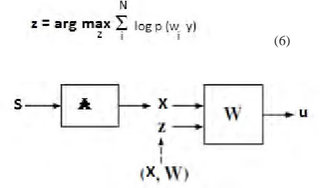
Where, components of u are as independent as possible. The underdetermined BSS problem is reported to be difficult to tackle than conventional, since some of the observations are hidden in the underdetermined case. For such condition short time Fourier transform or wavelet packet transform were also used. Kim S. and Chang D. (2003) proposed to convert the underdetermined BSS into conventional BSS by generating hidden observations z. The hidden observation ‘z’ is generated by maximizing their conditional probabilities given the observation X and the matrix W it is represented as,
(6)
Figure 4 Block diagram of underdetermined BSS by generating hidden observations
Where wi is the ith row of the matrix W and therefore wiy represents ui. As shown in Figure. 4, the sources are
a linear product of W and y as it remains in the case of conventional BSS.
u = Wy
(7)
2.4.Sparse ICA Approach:
Sparsity is also a major area of focus in case of ICA. A signal is said to be sparse when it is zero or nearly zero more than might be expected from its variance. Such a signal has a probability density function or distribution of values with a sharp peak at zero and fat tails. A standard sparse distribution is the Laplacian distribution, which has led to the sparseness assumption being occasionally referred to as a Laplacian prior. When ICA is used to extract features, the principle of maximum non-Gaussianity reflects the connection to sparse codingthat has been used in neuroscientific theories of feature extraction. The idea in sparse coding is to represent data with components so that only a small number of them are active at the same time. It turns out that this is equivalent, in some situations, to finding components that are maximally non-Gaussian [Mutihac R., Hulle M.(2004)]. The estimates provided by ICA are useful even when they are far from mutual independency because ICA also serves some other useful purposes than dependence reduction, such as projection pursuit and sparse coding. Another approach is two steps procedure in which the mixing matrix and the sources are estimated separately [Li Y., et al. (2003)]. If the sources are sufficiently sparse (i.e., they can be overlapped to some degree), blind separation can be carried out directly in the time domain. Otherwise, wavelet packets transformation preprocessing is necessary, and the blind separation is implemented in time-frequency domain. In another study [Jafari M., et al. (2006)], the convolutive blind source separation (BSS) problem with a sparse independent component analysis (ICA) method is addressed, which uses ICA to find a set of basis vectors from the observed data, followed by clustering to identify the original sources.
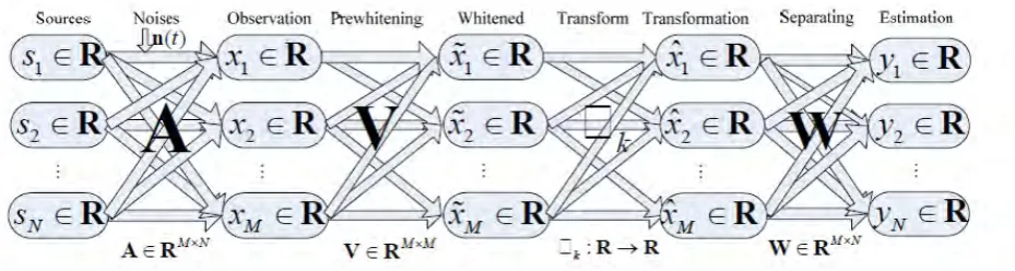
An innovative method called multiresolution subband Blind Source Separation (MRSBSS) methods has been discussed by some researchers. The definition of the same is given as “The MRSBSS can be formulated as a task of estimation of the mixing matrix on the basis of suitable multiresolution subband decomposition of sensors signals and by applying a classical BSS method(instead for raw sensor data) for one or several pre-selected sub bands for which source Sub-components are least dependent.” In [Li H., et al (2009)] different approaches to transformations of the source signals and various methods to choose the optimal subset of the coefficients in a set of MRSBSS algorithms are discussed. The whole procedure of the MRSBSS, from mixing to separating, is described in Figure 5. It further describes that Subband decomposition ICA (SDICA) an extension of ICA, assumes that each source is represented as the sum of some independent subcomponents and dependent subcomponents, which have different frequency bands.
Figure 5 The mixing – separation procedure of MRSBSS.
2.5.Noise scenario:
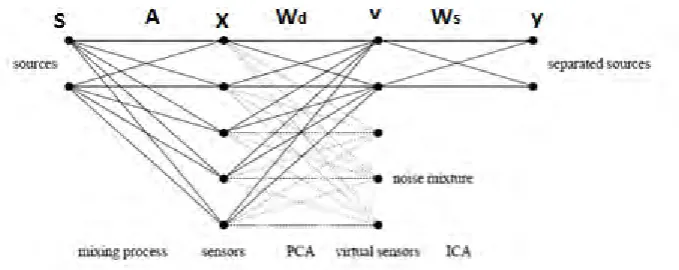
As has been discussed earlier, there exists another case of disparity between the number of sources & number of observation called over determined case. An approach is adapted in [Delfosse N. and Loubaton P.(2000)] to the case where the number of sensors is strictly greater than the number of sources. It illustrates an adaptive three-step procedure. A decomposed and normalized lattice synthesis filter is introduced. It solves the problem of singularity and as it is stable for any choice of its parameters, this filter can be adaptively computed and leads to a stable adaptive algorithm. In routine BSS problem, ideal sensors are usually assumed, which have no additive sensor noise. Only little work has been done on the analysis of algorithms in the case of noisy sensors. In [Joho M., et al. (2001)] concentration is focused on the case where a low SNR is present at the sensors, and shows that one possible way to enhance the performance of the separation is to use more sensors than source signals. The task is divided into two stages (Figure. 6 and 7). Starting with M input sensors, the first stage performs a singular-value decomposition Producing Ms virtual sensors (Ms < M), which still contain a noisy mixture of the source signals, but with a higher SNR than the true sensors. The remaining (M - Ms) virtual sensors contain a mixture of the sensor noises and are discarded in the second stage. The second stage consists of an ordinary blind source separation algorithm for the Ms X Ms problem.
Figure 6 Ideal BSS set up without noisy sensors
Figure 7 Over determined BSS problem divided into two stages
As discussed earlier; noise has also been a parameter of investigation of many scholars. The effect of noise on the separation process is discussed quite thoroughly by many authors. Rivet B., et al. (2004) illustrated the wavelet based denoising pre separating (P.S) processing in two ways. The paper has added that, the best performances of the ideal BSS model and their effectiveness are definitely decreased with observations corrupted by additive noise. In an instantaneous linear problem of source separation, the unknown source signals and the observed data are related by,
y(k) = AS(k) + n(k) = X(k) + n(k)
( 8 )
By estimating a q × p full rank matrix B one provides estimated sources which are the components (as independent as possible) of the output signal vector (k) defined as (Fig. 8):
(k) = B
y(k) =
BAS(k) + Bn(k)
( 9 )
Figure 8 Blind source separation model in noisy mixtures
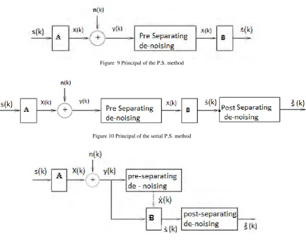
In the work two methods called serial & parallel P.S. are proposed & compared for denoising purpose. (Refer Figure. 9, 10 and 11).
Figure 9 Principal of the P.S. method
Figure 10 Principal of the serial P.S. method
Figure 11 Principal of the parallel P.S. method
The major problem of the first two methods in pre- separating case lies in the denoising processing which might remove the essential details & hence another principle is also proposed which have been claimed to differentiate the estimation of the separating matrix & the restoration of the denoised sources.
Another two-stage approach to extract high fidelity speech signals after BSS is studied. The proposed method considers an over-determined setting, where the number of sensors used is more than the speech signals to be separated. In other effort [Lie J., et al. (2009)], the spatial diversity is exploited to provide higher SINR improvement using MDNR (minimum distortion noise reduction) algorithm.
The source separation has unlimited areas of applications reported & are being explored. This technique is so useful & necessary that many researchers still trying to investigate newer areas, methods, techniques and approaches. Following section tries to focus on the current trends of the research going on.
3. Recent Developments:
The latest research presents an adaptive step-size method for blind source separation (BSS) suitable for robot audition systems has been proposed. [Nakajima H., et al. (2010)]. Also, comparison of traditional BSS methods over an incremental learning scheme (an online mode), on the basis of computational complexity & storage requirements [Zhou G., et al. (2011)] and [Kim T. (2011)] works are based on Frequency-domain blind source separation (BSS) techniques with the objective of increasing the speed and/or reducing the computational complexity of conventional algorithms, mainly for applications that involve large convolutive mixture filters.
Most of the proposed frequency-domain BSS structures are derived from the classic independent component analysis (ICA) algorithm. Some works have adopted different solutions, such as employing estimates of directions of arrival (DOA) or propagation delays. But in [Clark F., et al. (2011)] the combination of the binary-masking approach with the BSS high-order frequency dependencies algorithm is used for faster convergence and better perceptual quality. A new method of frequency domain is reported in [Nesta F. (2011)] where the problem of limitation of number of time observations for each frequency and increase in variation of ICA estimator is overcome with the help of recursively regularized implementation of ICA (RR-ICA). Another study [Wang L., et al. (2011)] proposes the convolutive blind source separation (BSS) problem that can be solved efficiently in the frequency domain, where instantaneous BSS is performed separately in each frequency bin.
Till now, the sources were supposed to be stationary but [Naqvi S., et al. (2010)] studies the visual modality to facilitate the separation for both stationary and moving sources and [Tang J., et al. (2010)] explores the concept of signal-to-noise ratio (MSNR) BSS assisted by complex wavelet transform to separate the individual; partial discharge among the mixed PD source signals concurrently occurring in a GIS pipe. A time domain work presented in [Kleinsteuber M. and Hao S. (2012)] deals with the problem of simultaneously separating and reconstructing signals from compressively sensed linear mixtures by combining compressive sensing with linear mixing which can be generalized further as Morphological Component Analysis.
The paper [Yoshioka T., et al. (2011)] proposes to perform BSS & blind dereverberation simultaneously. The proposed method uses a network, in which dereverberation and separation networks are connected in successive order, to estimate source signals.
4. Applications:
The researchers claim to find the blind source separation approach provides a significant improvement in the image reconstruction with the help of shape estimation [Fortuna J. and Martinez A.(2006)]. Out of many applications reported, the BSS techniques proved useful for the analysis of multivariate data sets such as financial time series, astrophysical data sets, electrical and hemodynamic recordings from the human brain and digitized natural images. It also enjoys various applications in structural dynamics, including damage detection, condition monitoring, biomedicine, speech, signal processing, and discrimination between pure tones and sharp-pointed resonances and more recently also to time series forecasting using stock data [Ponceleta F., et al. (2007)]. Another interesting application [Olyaee S., et al. (2010)] deals with the problem of the multisource limitation of the nutating rising-sun reticle based optical trackers.
The source separation problem is of interest in various applications such as the localization and tracking of targets using radars and sonars, separation of speakers (problem known as “cocktail party”), detection and separation in multiple-access communication systems, independent component analysis of biomedical signals (EEG or ECG), multispectral astronomical imaging, geophysical data processing, Typical examples are mixtures of simultaneous sounds or human voices that have been picked up by several microphones, brain signal measurements from multiple EEG sensors, several radio signals arriving at a portable phone, or multiple parallel time series obtained from some industrial process, multipath propagation in mobile communications, and separation of QAM sources, Medical signal processing, Industrial problems, such as fault detection, Extraction of meaningful features from data,earth science, and applied sciences [Oja E., et al. (2006) , Karhunen J., et al.(1997), Lin S. and Tung P. (2006)].
The BSS ICA module finds its wide area application in other the fields like satellite communications; radio-mobile communications in the context of the space division multiple access (SDMA) mode; array calibration; and use of visual signals for speech enhancement, audiovisual source Separation, signal encryption, micro-array data analysis, multi-spectrum image processing. [Delfosse N. and Loubaton P.(2000), Rivet B., et al. (2007), and Casanovas A., et al. (2007)].
5. Conclusion:
It is still hard to appraise an algorithm or to compare several algorithms because of the lack of suitable performance measures and common test, even in the very simple case of linear instantaneous mixtures. A lot of BSS models such as instantaneous linear mixtures, convolutive mixtures are presented in recent publications. The real world observations are often mixtures of different signals plus noise and researchers in different application areas try to develop methods that can blindly estimate the original sources.
In the early phase the focus was on the comparison of time domain & frequency domain approaches. In majority of cases it has been pointed out that the time domain approach is most significant while separating process can be carried out. The second phase of the research has concentrated on the sparsity of the signal & time-frequency analysis. The advantage of a sparse signal representation is that the probability of two or more sources being simultaneously active is low. Thus, sparse representations lend themselves to good separability because most of the energy in a basis coefficient at any time instant belongs to a single source. Additionally, sparsity can be used in many instances to perform source separation in the case when there are more sources than sensors. The sparsity has been utilized efficiently & the time frequency analysis has given new dimensions to the separation issues.
6. References:
[1] Simon Haykin : Neural networks 2nd edition, Prentice Hall, 1999
[2] C. Jutten, Calcul neuromimétique et traitement du signal: analyse en composantes ndépendantes,Thèse d’état ès sciences physiques, UJF-INP Grenoble, 1987
[3] Juha Karhunen: Neural approaches to independent component analysis & source separation, Helsinki university of technology, 1999
[4] S. Amari and A. Cichocki. Adaptive blind signal processing - neural network approaches. Proceedings IEEE, 86:1186–1187, 1998.
[5] S. Amari, A. Cichocki, and H.H. Yang. A new learning algorithm for blind signal separation., Advances in Neural Information Processing Systems 1995, volume 8, pages 757–763. MIT Press: Cambridge, MA, 1996.
[6] [6] Pierre Comon and Christian Jutten: BLIND SOURCE SEPARATION, Published by Elsevier Ltd, 1996.
[7] J. Basak and S.-I. Amari : Blind separation of uniformly distributed signals: A general approach. IEEE Trans. On Neural Networks, 10(5):1173–1185, 1999.
[8] P. Comon, Independent Component Analysis. Republished in Higher-Order Statistics, Elsevier,pp. 29–38. 1992. [9] P. Comon, Independent component analysis, a new concept? Signal Process. 287–314, 1994
[10] Saeed Olyaee, Mohammad Shams Esfand Abadi, Reza Ebrahimpour and Mohammad Reza Moradian: A Comparative Study of Two Blind Source Separation Approaches to Resolve the Multi-Source Limitation of the Nutating Rising-Sun Reticle Based Optical Trackers, International Journal of Computer and Electrical Engineering, Vol. 2, No. 2, April, 1793-8163, 2010
[11] Shih-Lin Lin, Pi-Cheng Tung : A Modified Method for Blind Source Separation, , Proceedings of the 6th WSEAS International Conference on Applied Computer Science, Tenerife, Canary Islands, Spain, December 16-18, 2006
[12] Shoko Araki,Shoji Makino,Ryo Mukai,Tsuyoki Nishikawa, Hiroshi Saruwatari : Fundamental Limitation Of Frequency Domain Blind Source Separation For Convolved Mixture Of Speech., IEEE Trans. Speech Audio Process, 2001
[13] Kamran Rahbar, James P. Reilly : A New Frequency Domain Method for Blind Source Separation of Convolutive Audio Mixtures., 2002
[14] F. Ponceleta, G. Kerschena,_, J.-C. Golinval, D. Verhelst: Output-only modal analysis using blind source separation techniques, Mechanical Systems and Signal Processing, p.p.2335–2358, 2007
[15] Jeff Fortuna and Aleix M. Martinez: A Blind Source Separation Approach to Structure From Motion, Department of Electrical & Computer Engineering, The Ohio State University, 2006
[16] J.M. Gorriz, C.G. Puntonetb, F. Rojasb, R. Martinc, S. Hornilloc, E.W. Lang : Optimizing blind source separation with guided genetic algorithms , ELSEVIER, Neurocomputing 69, 1442–1457,2006
[17] Ying Tan, and Jun Wang: Nonlinear Blind Source Separation Using Higher Order Statistics and a Genetic Algorithm:, Transactions on evolutionary computation, vol. 5, no. 6, December 2001
[18] Kenji Nakayama Akihiro Hirano Takayuki Sakai: An Adaptive Nonlinear Function Controlled by Kurtosis for Blind Source Separation, IEEE, 2002
[19] Chun-Hou Zheng, Zhi-Kai Huang, Michael R. Lyu, and Tat-Ming Lok, J. Wang : Nonlinear Blind Source Separation Using Hybrid Neural Networks,(Eds.): ISNN 2006, LNCS 3971, pp. 1165 – 1170, 2006.
[20] C.S. Rai , Yogesh Singh: Source distribution models for blind source separation,ELSEVIER, Neurocomputing, 57, 501 – 505, 2004
[21] Yogesh Singh,C.S. Rai : Blindsource separation: A Unified Approach, ELSEVIER, Neurocomputing 49, 435 – 438,2002 [22] Yogesh Singh, C. S. Rai : A simplified approach to independent component analysis,Neural Computers & Applications, 173–
177,2003
[23] Juha Karhunen, Aapo Hyvarinen, Ricardo Vagcirao, Jarmo Hurri and Erkki Oja: Applications Of Neural Blind Separation To Signal And Image Processing, IEEE, PP 131-134,1997
[24] Shun-Ichi Amari, And Andrzej Cichocki: Adaptive Blind Signal Processing—Neural Network Approaches, proceedings of the IEEE, vol. 86, no. 10, October 1998
[25] Abdeldjalil A¨ıssa-El-Bey, Karim Abed-Meraim, and Yves Grenier : Underdetermined Blind Audio Source Separation Using Modal Decomposition,EURASIP Journal on Audio, Speech, and Music Processing, , Article ID 85438, Volume 2007.
[26] Sanggyun Kim and Chang D. Yoo: Blind Separation of Speech and Sub-Gaussian Signals in Underdetermined Case, 2003. [27] Qiu-Hua Lin, Fu-Liang Yin, Tie-Min Mei, and Hualou Liang: A Blind Source Separation Based Method for Speech Encryption,
IEEE Transactions On Circuits And Systems—i: Regular Papers, vol. 53, no. 6, June 2006
[28] R. Mutihac, Marc M. Van Hulle : Comparison Of Principal Component Analysis And Independedent Component Analysis For Blind Source Separation, Romanian Reports in Physics, Volume 56, Number I, P. 20-32, 2004
[29] Yuanqing Li, Andrzej Cichocki and Shun-ichi Amari: Sparse Component Analysis For Blind Source Separation With Less Sensors Than Sources, 4th International Symposium on Independent Component Analysis and Blind Signal Separation (ICA2003), , Nara, Japan, April 2003
[30] Maria G. Jafari, Samer A. Abdallah, Mark D. Plumbley, and Mike E. Davies, Sparse Coding for Convolutive Blind Audio Source Separation, Springer-Verlag Berlin Heidelberg, 2006
[31] Hongwei Li, Rui Li, Fasong Wang : Multiresolution Subband Blind Source Separation: Models and Methods, Journal of Computers, vol. 4, no. 7, July 2009
[32] Prof. Patrick Wolfe: DUET Algorithm for Blind Source Separation, ES 257 Advanced Speech and Audio Processing, May 18, 2005
[33] Nathalie Delfosse and Philippe Loubaton, Member, IEEE: Adaptive Blind Separation of Independent Sources: A Second-Order Stable Algorithm for the General Case, IEEE transactions on circuits and systems—I: fundamental theory and applications, vol. 47, no. 7, July 2000.
[34] Marcel Joho, Heinz Mathis, and Russell H. Lambert: Overdetermined Blind Source Separation: Using More Sensors Than Source Signals In A Noisy Mixture, 2001
[35] Bertrand Rivet, Vincent Vigneron, Anisoara Paraschiv-Ionescu and Christian Jutten: Wavelet de-noising for blind source separation in Noisy mixtures. 2004
[36] J. P. Lie, F. Sattar, C. M. S. See,A. K. Kattepur: High Fidelity Blind Source Separation Of Speech Signals,17th European Signal Processing Conference (EUSIPCO 2009) Glasgow, Scotland, August 24-28, 2009
[38] Guoxu Zhou, Zuyuan Yang, Shengli Xie, and Jun-Mei Yang : Online Blind Source Separation Using Incremental Nonnegative Matrix Factorization with Volume Constraint, IEEE transactions on neural networks, vol. 22, no. 4, April 2011
[39] Taesu Kim : Real-Time Independent Vector Analysis for Convolutive Blind Source Separation, , IEEE transactions on circuits and systems—I: regular papers, vol. 57, no. 7, July 2010
[40] Felipe S. P. Clark, Mariane R. Petraglia, and Diego B. Haddad : A New Initialization Method for Frequency-Domain Blind Source Separation Algorithms, IEEE signal processing letters, vol. 18, no. 6, June 2011.
[41] Francesco Nesta,Piergiorgio Svaizer, and Maurizio Omologo : Convolutive BSS of Short Mixtures by ICA Recursively Regularized Across Frequencies, IEEE transactions on audio, speech, and language processing, vol. 19, no. 3, March 2011. [42] Lin Wang, Heping Ding, and Fuliang Yin: A Region-Growing Permutation Alignment Approach in Frequency-Domain Blind
Source Separation of Speech Mixtures, IEEE transactions on audio, speech, and language processing, vol. 19, no. 3, March 2011 [43] Syed Mohsen Naqvi, Miao Yu, and Jonathon A. Chambers: A Multimodal Approach to Blind Source Separation of Moving
Sources, IEEE journal of selected topics in signal processing, vol. 4, no. 5, October 2010
[44] Ju Tang, Wei Li, and Yilu Liu: Blind Source Separation of Mixed PD Signals Produced by Multiple Insulation Defects in GIS,IEEE transactions on power delivery, vol. 25, no. 1, January 2010
[45] Martin Kleinsteuber, Member, IEEE, and Hao Shen : Blind Source Separation With Compressively Sensed Linear Mixtures, IEEE signal processing letters, vol. 19, no. 2, February 2012
[46] [46] Takuya Yoshioka, Tomohiro Nakatani, Masato Miyoshi, and Hiroshi G. Okuno,: Blind Separation and Dereverberation of Speech Mixtures by Joint Optimization, IEEE transactions on audio, speech, and language processing, vol. 19, no. 1, January 2011
[47] Min Jing, T. Martin McGinnity,Sonya Coleman, Huaizhong Zhang, Armin Fuchs, and J. A. Scott Kelso : Enhancement of Fiber Orientation Distribution Reconstruction in Diffusion-Weighted Imaging by Single Channel Blind Source Separation, IEEE transactions on biomedical engineering, vol. 59, no. 2, February 2012
[48] Erkki Oja, Juha Karhunen, Alexander Ilin, Antti Honkela, Karthikesh Raju, Tomas Ukkonen, Zhirong Yang, Zhijian Yuan: Independent component analysis and blind source separation, 2006
[49] Bertrand Rivet, Laurent Girin, and Christian Jutten, Mixing Audiovisual Speech Processing and Blind Source Separation for the Extraction of Speech Signals From Convolutive Mixtures, IEEE transactions on audio, speech, and language processing, vol. 15, no. 1, January 2007