https://doi.org/10.5194/amt-11-6309-2018 © Author(s) 2018. This work is distributed under the Creative Commons Attribution 4.0 License.
CALIPSO lidar calibration at 532 nm: version 4 daytime algorithm
Brian J. Getzewich1, Mark A. Vaughan2, William H. Hunt1,†, Melody A. Avery2, Kathleen A. Powell2, Jason L. Tackett1, David M. Winker2, Jayanta Kar1, Kam-Pui Lee1, and Travis D. Toth2
1Science Systems and Applications Inc., Hampton, Virginia, USA 2NASA Langley Research Center, Hampton, Virginia, USA †deceased
Correspondence:Brian J. Getzewich ([email protected]) Received: 25 June 2018 – Discussion started: 7 August 2018
Revised: 5 November 2018 – Accepted: 6 November 2018 – Published: 22 November 2018
Abstract.The Cloud Aerosol Lidar and Infrared Pathfinder Satellite Observations (CALIPSO) mission released version 4.00 of their lidar level 1 data set in April of 2014, and sub-sequently updated this to version 4.10 in November of 2016. The primary difference in the newly released version 4 (V4) data is a suite of updated calibration coefficients calculated using substantially revised calibration algorithms. This paper describes the revisions to the V4 daytime calibration proce-dure for the 532 nm parallel channel. As in earlier releases, the V4 daytime calibration coefficients are derived by scal-ing the raw daytime signals to the calibrated nighttime sig-nals acquired within a calibration transfer region, and thus the new V4 daytime calibration benefits from improvements made to the V4 532 nm nighttime calibration. The V4 cali-bration transfer region has been moved upward from the up-per troposphere to the more stable lower stratosphere. The identification of clear-air columns by an iterative threshold-ing scheme, crucial to selectthreshold-ing the observation regions used for calibration, now uses uncalibrated 1064 nm data rather than recursively using the calibrated 532 nm data, as was done in version 3 (V3). A detailed account of the rationale and methodology for this new calibration approach is pro-vided, along with results demonstrating the improvement of this calibration over the previous version. Extensive valida-tion data acquired by NASA’s airborne high spectral reso-lution lidar (HSRL) shows that during the daytime the av-erage difference between collocated CALIPSO and HSRL measurements of 532 nm attenuated backscatter coefficients is reduced from 3.3 %±3.1 % in V3 to 1.0 %±3.5 % in V4.
1 Introduction
The Cloud-Aerosol Lidar with Orthogonal Polarization (CALIOP), on-board the Cloud-Aerosol Lidar and Infrared Pathfinder Satellite Observations (CALIPSO) satellite, has been providing a near-continuous record of high-resolution vertical profiles of clouds and aerosols since the summer of 2006. Launched 28 April 2006, CALIPSO is an integral part of the NASA’s Afternoon (A-Train) constellation, working in tandem with other Earth observing satellites to probe the nature and influence of clouds and aerosols on the global cli-mate system (Winker et al., 2010). CALIOP is a dual wave-length, polarization-sensitive elastic backscatter lidar pow-ered by an Nd : YAG diode-pumped laser that makes range-resolved measurements of the total backscatter intensity at 1064 nm and the 532 nm backscatter intensities in planes ori-ented parallel and perpendicular to the polarization plane of the transmitted laser beam (Hunt et al., 2009). Among the first of its kind, and having delivered the longest duration of continuous on-orbit operations, CALIOP provides unique insights into the vertical distribution, morphology and vari-ability of clouds and aerosols (Chand et al., 2009; Vernier et al., 2011; Forbes and Ahlgrimm, 2014; Tan et al., 2016; Stephens et al., 2018).
tech-nique (Russell et al., 1979; Powell et al., 2009; Kar et al., 2018), in which calibration coefficients are determined by taking the ratio of the measured signal to the expected sig-nal computed using an atmospheric model. This approach as-sumes that all constituents of the nighttime normalization re-gion (i.e., including aerosol loading) can be accurately mod-eled or characterized. The same technique cannot be used during daytime, however, because the SNR is substantially lower due to the influence of the reflected solar background radiation. This is rectified by scaling the daytime to the night-time calibration by using clear air attenuated scattering ra-tios, defined as the ratio between the measured attenuated backscatter and modeled molecular signal. These are mea-sured and accumulated over identical altitude ranges and lat-itude bands during both daytime and nighttime. The funda-mental assumption for the 532 nm daytime calibration proce-dure is that a persistent “calibration transfer region” can be identified where the aerosol loading remains diurnally invari-ant over relatively short periods of time (e.g., 7–10 days).
Calibration algorithms used in the version 3 (V3) series of L1 data products (Vaughan et al., 2018), released begin-ning in June 2009 are described in Hostetler et al. (2005); Powell et al. (2008, 2009, 2010); and Vaughan et al. (2010). Over the intervening years since the release of V3, several shortcomings have been identified in the 532 nm daytime cal-ibration algorithm. First, the altitude of the V3 calcal-ibration transfer region was too low, and hence the assumed diurnal invariance for the 532 nm daytime calibration was often not satisfied, as noted in Powell et al. (2010) and described fur-ther in Sect. 2. Frequent cloudiness at tropical latitudes also limited the number of clear-air samples available at this alti-tude range. Second, identifying the cloud-free data segments needed to calculate the V3 daytime calibration coefficients was accomplished by repeatedly generating a subset of the lidar level 2 (L2) products, and this interdependency prohib-ited the independent calculation of the 532 nm daytime cali-bration coefficients. Finally, the calculation of the calicali-bration uncertainty estimates in V3 failed to accurately include all error sources associated with the approach.
To account for these identified weaknesses in the V3 al-gorithm, the CALIPSO project completely redesigned the calibration architecture for the version 4 (V4) L1 data prod-ucts. The 532 nm nighttime calibration has been updated to accommodate a change in the molecular normalization re-gion in the stratosphere from 30–34 to 36–39 km (Kar et al., 2018). This change was based on a better understanding of the vertical distribution of stratospheric aerosols (Vernier et al., 2009). As for the 532 nm daytime calibration, which is the focus of this paper, the technique still relies on match-ing daytime and nighttime clear air scattermatch-ing ratios, but with several crucial modifications that address the problems iden-tified above. An overview of the V3 calibration procedure is provided in Sect. 2, followed by a detailed summary of the new V4 method in Sect. 3. Section 3 fully describes the up-dated assumptions and new techniques used in V4. Section 4
compares the V4 calibration coefficients against internally established scientific metrics used to assess the performance of the algorithm. Section 4 also updates a previous compari-son between CALIOP V3 backscatter coefficients and exten-sive collocated measurements from the NASA Langley Re-search Center (LaRC) airborne high spectral resolution lidar (HSRL) (Rogers et al., 2011). Some concluding remarks are given in Sect. 5.
2 Version 3 532 nm daytime calibration
The V3 532 nm daytime calibration procedures transfer the 532 nm parallel channel nighttime calibration to the daytime measurements (Powell et al., 2010). Calibrating the daytime signals relative to the nighttime measurements is done for two reasons: (a) low SNR during the daytime prevents cali-bration using the high-altitude molecular normalization tech-nique, and (b) thermally induced changes in the alignment of the laser transmitter with respect to the receiver produce sub-stantial changes in the daytime calibration over the course of each daytime orbit segment. Transferring calibration from nighttime to daytime was accomplished in V3 by using lati-tudinally varying clear-air attenuated scattering ratios, accu-mulated for both day and night orbital segments, to derive correction factors associated with the along-track misalign-ments that occur during the daytime. For any daytime gran-ule, the 532 nm daytime calibration coefficients were then computed as the product of a mean correction factor built from an accumulation of several days’ worth of scattering ra-tios (discussed further in this section) and the mean 532 nm calibration coefficient from the previous nighttime granule (Powell et al., 2010).
The attenuated scattering ratios,R0, are defined as the ra-tio between the measured total attenuated backscatter coef-ficients,βmeasured0 , and a profile of modeled molecular atten-uated backscatter coefficients,βmodel0 , derived from modeled profiles of temperature and pressure (Powell et al., 2009), as given by
R0(z)=β 0
measured(z)
βmodel0 (z)
= Xtotal/Ce
βmodel,m(z) Tmodel2 ,m(z) Tmodel2 ,O3(z)
. (1)
In this expression the subscripts m and O3represent, respec-tively, contributions from molecular and ozone scattering and attenuation.Ceis the estimated 532 nm total calibration coef-ficient,βm(z)is the molecular backscatter coefficient at alti-tudez,T2(z)is the two-way transmittance between the lidar and altitudez, andXtotalis the range corrected, gain and en-ergy normalized total backscatter signal at 532 nm (i.e., the sum of the parallel and perpendicular components), such that
Xtotal(z)=
r(z)2 E
!
Pk(z)
Gk +
P⊥(z) G⊥PGR
wherer(z)is the range from the lidar to altitudez, andEis the laser pulse energy.Pk(z)andP⊥(z)are, respectively, the 532 nm signals measured in the parallel and perpendicular channels,GkandG⊥are the electronic gains of the respec-tive receiver channels, and PGR is the polarization gain ratio, i.e., “the ratio ofP⊥(z)toPk(z)when both channels are illu-minated by the same light levels” (Hunt et al., 2009; Powell et al., 2009).
The nighttime and daytime clear-air attenuated scattering ratios in V3 are calculated for “frames” of data within the calibration transfer region. Each frame extends for 200 km along-track at an altitude of 8 to 12 km. The 8 to 12 km alti-tude range was chosen to be high enough to avoid substantial diurnal variation of the aerosol loading in the lower tropo-sphere and low enough to provide relatively robust SNR, thus minimizing the influences of solar background radiation on the daytime signal. The clear-air attenuated scattering ratios in the V3 8–12 km calibration transfer region were assumed to be diurnally invariant. Based on this assumption, initial es-timates of the mean attenuated scattering ratios,R0
day,initial, are calculated for each daytime frame using the mean of the 532 nm calibration coefficients,Cenight, computed during the previous nighttime granule; i.e.,
R0
day,initial= *
Xtotal,day zj, pk
e
Cnightβmodel0 ,day zj, pk +
. (3)
Here the angle brackets indicate averaging over all altitudes
zj between 8 and 12 km for all profilespk lying within the
daytime clear-air calibration transfer region. For each night-time clear-air region, the mean clear-air attenuated scattering ratios, R0night, are calculated using the same formula as in
Eq. (3), except using the nighttime signals, gain settings, and calibration coefficients.
Initial correction factor estimates,Winitial, are then derived by using the mean attenuated scattering ratios residing in cor-responding latitudes of the day–night calibration transfer re-gions of the orbits, as seen in Eq. (4):
Winitial=
Rday0 ,initial
R0night . (4)
The 532 nm daytime calibration procedure generates daily estimates of correction factors built from a moving averag-ing window of the day and night clear-air attenuated scat-tering ratios accumulated over the previous 7 days. A mini-mum window size of 4 days is required in case of instrument downtime or the inability to downlink data. Looking back-wards and not including current scattering contributions for the orbit that is being calibrated are both required because the L2 5 km cloud and aerosol layer data products are needed to identify the clear air regions. These daily correction factors are smoothed onto a 1◦ latitude window and reported as a function of elapsed seconds,W (t ), from the start of a refer-ence orbit that reflects the general orbital configuration for
that day (i.e., time will differ from latitude based on time of year). Additional filtering and smoothing are applied to mit-igate outliers. In particular, a minimum nighttime scattering ratio of 1.03 is used to compensate for diurnal differences in aerosol loading in the troposphere (Powell et al., 2010). Selection of this offset was based on observational analysis during development of the V3 algorithm, where it was noted that zonal distributions of attenuated scattering ratios in the calibration transfer regions fell below 1.0 in the tropics. This dip in the nighttime scattering ratios is attributed to signal at-tenuation by undetected cloud and aerosol layers in the upper troposphere (e.g., Vernier et al., 2009).
To construct valid sets of correction factors, the data frames used in the V3 daytime calibration procedure must consist entirely of “clear air” from the top of the lidar return at 40 km down to the base of the V3 calibration transfer re-gion at 8 km. Note that, in this context, “clear air” does not imply a pristine, aerosol-free molecular atmosphere. Instead, we impose the requirement that no layers are detected within this region by the CALIOP multi-resolution layer detection algorithm (Vaughan et al., 2009). Any undetected residual aerosol is assumed to be diurnally invariant. For the cali-brated nighttime data, the required clear air frames can be identified directly from the automatically generated L2 data products. But because the layer detection algorithm requires calibrated L1 data for its operation, determining daytime clear air frames requires an intermediate operation, wherein the layer detection module is embedded in an iterated opti-mization loop initiated using a coarse first approximation to the daytime calibration scale factors. These scale factors are subsequently refined through successive iterations. At each step, the required regions of “clear air” are identified by ap-plying the layer detection procedure to the current estimate of the daytime attenuated scattering ratios, which are derived by applying the most recent iteration of the daytime cali-bration scale factors. The final correction factor curves are stored in internal ancillary lookup tables. The 532 nm day-time calibration coefficients are derived by multiplying these time-varying correction factors by the mean of the previous granule’s 532 nm nighttime calibration coefficient, as shown in Eq. (5), wheretrepresents granule-elapsed time; i.e.,
Cday(t )=W (t ) Cnight. (5)
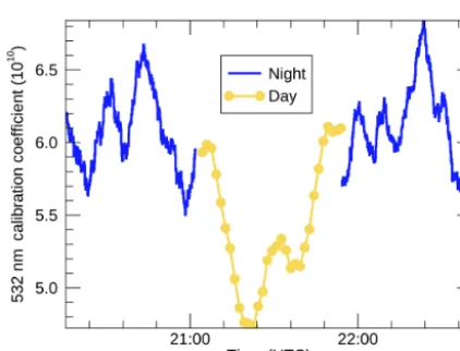
Figure 1. V3.40 532 nm calibration coefficients between succes-sive CALIPSO night–day–night orbits on 18 December 2016 from 20:15:31 to 22:40:41 UTC.
3 Version 4 532 nm daytime calibration
The fundamental assumption underlying the V4 532 nm day-time calibration scheme is the same one invoked in V3; i.e., the mean attenuated scattering ratios do not vary signifi-cantly during a diurnal cycle within a defined region in the atmosphere, and hence the mean uncalibrated daytime at-tenuated scattering ratios can be scaled to match the mean nighttime attenuated scattering ratios in this calibration trans-fer region. Here we list the major changes between the V3 and V4 daytime calibration algorithms. First, two new signal adjustments have been incorporated into the L1 processing, and these have a small but direct impact on the subsequently derived calibration coefficients. Second, the selection of the calibration transfer region has been changed so that a 400 K potential temperature isotherm in the lower stratosphere now defines the bottom of the vertical calibration range, replacing the fixed altitude cross-tropopause region used in V3. Third, a newly developed multi-granule averaging scheme compen-sates for the reduced SNR incurred by moving the calibration transfer region upwards. To further boost the SNR, rather than using the total signal (i.e., parallel plus perpendicular, as in Eq. 2), only the parallel channel is considered. Fourth, the V4 procedure uses a modified version of the L2 layer de-tection algorithm to search the uncalibrated 1064 nm chan-nel backscatter coefficients for clear air regions, instead of using the calibrated 532 nm attenuated scattering ratios, as was done in V3. This eliminates the need for a multi-pass architecture, and has two major benefits. The revised V4 cal-culations are more transparent, making it easier for external data users to replicate and/or validate the calibration coeffi-cients and uncertainties reported in the V4 L1 data products. Also, by eliminating the recursive process, the V4 scheme significantly reduces the number of processing steps required to generate the resultant data product. Fifth and finally, the
V4 532 nm daytime calibration coefficients uncertainties are computed directly from the nighttime calibration coefficient uncertainties, using the calibrated 532 nm nighttime and un-calibrated 532 nm daytime attenuated scattering ratios. In-creased accuracy in computing the 532 nm daytime calibra-tion coefficient uncertainties for V4 was also important, as a better understanding of the key contributors to the overall error was crucial in driving the averaging decisions used to calibrate all three channels. Each of these five algorithm up-dates is discussed in detail in the subsections below.
3.1 Signal adjustments
The V4 calibration procedure applies two new corrections to the daytime signal prior to the calibration: an adjustment to remove photomultiplier (PMT) baseline shapes and an updated day-to-night gain ratio. The motivation and imple-mentation of these two corrections are discussed in the para-graphs below.
The output of PMTs exposed to constant background light (e.g., sunlight reflected from dense water clouds) typically increases with time after the PMT is gated on, thus generat-ing a signal-induced baseline shape that varies as a function of the background light level. Prior to launch, the baseline shapes for the CALIOP detectors were repeatedly measured in the laboratory, and the magnitudes of the required signal adjustments were found to be quite small relative to the atmo-spheric signals typically measured in the troposphere. Con-sequently, because the prelaunch daytime calibration strat-egy was simply to interpolate daytime calibration coeffi-cients between neighboring nighttime molecular normaliza-tions (Hostetler et al., 2006; Powell et al., 2008), baseline shape corrections were deemed to be unnecessary and thus were not implemented. This assessment changed with the V4 redesign of the daytime calibration algorithms. The V4 daytime calibration relies on highly averaged daytime mea-surements in the middle-to-lower stratosphere where the ex-pected molecular signals are substantially weaker, and hence biases due to baseline shape artifacts are potentially signifi-cant. To mitigate these concerns, we used prelaunch labora-tory measurements together with post-launch extended back-ground measurements acquired periodically throughout the mission to characterize the PMT baseline shapes:
shape(z, B)=(zoffset−z)
X1B+X2B2
10G/20. (6) This approximation is a function of both altitude (z) and the measured background light intensity (B) atz=zoffset, where
ampli-fier gain. Shape correction profiles are computed on a shot-by-shot basis and applied to all data acquired during daytime measurements.
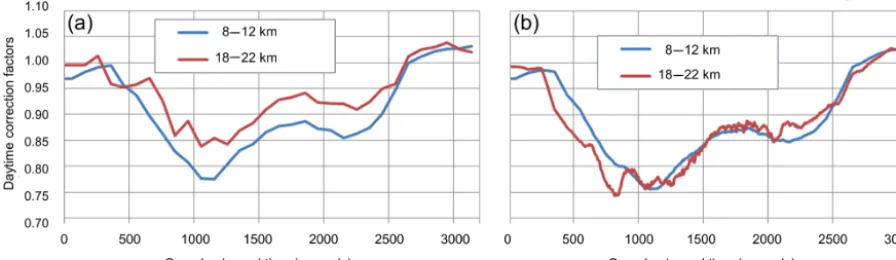
The improvements achieved by the application of the shape correction are illustrated in Fig. 2, which shows a 7-day average (13–19 December 2011) of the 7-daytime correc-tion factors derived using the V3 algorithm as a funccorrec-tion of orbital elapsed time for both the 8–12 km (V3 calibration transfer region) and an elevated 18–22 km region (an approx-imate V4 calibration transfer region for this time period). Figure 2a shows that there is a difference of up to 8 % in the correction factors between these two altitude levels, par-ticularly in mid-latitudes where bright clouds generate higher background signals. This difference as a function of altitude should not occur. By applying the V4 baseline shape correc-tion for this case in Fig. 2b, the correccorrec-tion factors, though slightly reduced, are now more similar. Although applying the shape correction causes an overall reduction in the appar-ent signal with increased altitude, the corrected signal more accurately corresponds to the atmospheric signal and elim-inates systematic artifacts in the daytime calibration coeffi-cients.
To prevent saturation of the digitizers by large daytime noise excursions, a fixed reduction in the detector gains is applied to all three channels during daytime operations. To compensate for these gain changes, the CALIOP calibra-tion routine applies fixed to-night gain ratios to the day-time measurements. On-orbit performance metrics and rou-tine built-in test system (BITS) measurements (Hunt et al., 2009) suggested that the 532 nm perpendicular and parallel day-to-night gain ratios needed to be increased by 0.65 % and 3.3 %, respectively. Though large, the 532 nm parallel adjust-ment has essentially no impact on the calibrated 532 nm day-time attenuated backscatter coefficients, because the gain in-crease is absorbed as a multiplicative factor into the calcu-lated calibration coefficients. Similarly, because the V4 day-time calibration only uses the signals from the parallel chan-nel, changes to the 532 nm perpendicular day–night gain ra-tios have no impact on the derived calibration, though they will ultimately yield a small increase in the 532 nm perpen-dicular and total attenuated backscatter coefficients reported in the L1 data products.
3.2 Revised calibration transfer region
The selection of the calibration transfer region is subject to two competing interests. Diurnal variation in background aerosol should be minimized, which argues for a higher alti-tude since, to first order, aerosol concentrations and diurnal variability tend to decrease with height. However, absent any aerosol loading CALIOP’s SNR also decreases with height, and obtaining an accurate calibration requires sufficient sig-nal to overcome the daytime background noise due to sun-light. The V3 algorithm approach maximized SNR, as pre-viously discussed, by choosing a calibration transfer region
with a fixed base of 8 km and a constant depth of 4 km (12 km top). However, this altitude domain occurs in the tropical tro-posphere where the CALIOP signal is frequently attenuated due to persistent cloud cover, and therefore has a reduced number of clear-air samples. There is also the possibility of potential contamination by clouds and aerosols not identi-fied by the L2 feature detection technique used to isolate clear air. In the extra-tropics, 8–12 km altitude range strad-dles the tropopause, where there is additional background aerosol variability caused by fluctuations in the tropospheric jet locations (Gettleman and Wang, 2015; Manney and Heg-glin, 2018). By elevating the calibration transfer region from the near tropopause into the lower stratosphere, the V4 ap-proach attempts to improve the fidelity of the clear-air attenu-ated scattering ratios by substantially reducing the possibility of any diurnal variability of background aerosol. Relocating to the lower stratosphere also minimizes the need for a robust feature detection algorithm to identify clear-air, as by defini-tion this more stable region contains fewer cloud and aerosol layers than are found in the troposphere. The trade off, as already noted, is a reduction in SNR that dictates more sam-pling, which will be discussed in more detail in Sect. 3.3.
Figure 2.The 532 nm daytime correction factor for 13–19 December 2011 based on the V3 L1 algorithm. The correction factor is computed for both the V3 calibration transfer region (8–12 km) and an elevated transfer region (18–22 km) without(a)and with(b)the baseline shape correction applied to the signal.
Two additional safeguards are used to avoid possible con-tamination of the clear-air attenuated scattering ratios. First, to both guard against features intruding into the lower strato-sphere, and because the algorithm uses a climatological monthly mean 400 K surface as the lower limit, an additional altitude offset of 2 km is applied to further elevate the base of the calibration transfer region. Secondly, since the strato-sphere is not entirely devoid of features, the algorithm em-ploys a 1064 nm feature detection technique, as discussed in Sect. 3.4, to exclude cloud and aerosol layers from the cali-bration averaging scheme. In particular, the presence of un-detected polar stratospheric clouds (PSCs) in the calibration transfer regions can introduce high biases into the calibration coefficient estimates. The potential impacts of feature con-tamination of the calibration transfer regions are discussed in detail in Sect. 4.2 and 4.3.
At the time of the V4 algorithm development and deploy-ment, GMAO provided an updated meteorological reanalysis product, MERRA-2 (Modern-Era Retrospective analysis for Research and Applications, Version 2) (Gelaro et al., 2017), which includes Microwave Limb Sounder (MLS) temper-atures and is a marked improvement over earlier GMAO-FPIT products. This new meteorological data was incorpo-rated into the V4.10 L1 and L2 data products, but was not used to re-compute the 400 K altitudes used by the 532 nm daytime calibration algorithm to set the calibration transfer region base altitude.
3.3 Mitigation of reduced SNR
Because the dominant source of noise during daytime opera-tions is the solar background signal, daytime SNR scales ap-proximately linearly with signal strength (Hunt et al., 2009). Moving the calibration region upward from a midpoint of 10 km in V3 to a nominal midpoint of∼20 km in V4 lowers the magnitude of the molecular attenuated backscatter coef-ficients in the calibration transfer region, and hence the SNR, by a factor of∼5. To compensate for this significant
reduc-tion in the SNR at the higher calibrareduc-tion altitudes, the number of frames averaged in V4 must increase when compared with V3. Furthermore, because daytime SNR scales as the square root of the number of frames averaged, maintaining the same calibration SNR in V4 that was achieved in V3 requires the V4 procedure to accumulate ∼25 times more frames than were used in V3. Given that each frame extends for 200 km along-track, this increase in sample size cannot be accom-plished within a single granule. Accurately characterizing the magnitude and rate of change of the daytime calibration co-efficients within the V4 algorithm therefore requires averag-ing across-track over multiple consecutive daytime granules. Applying standard propagation of errors techniques to the daytime calibration equations shows that an averaging period of 105 consecutive orbits (i.e., over 7 days), centered on the orbit to be calibrated, should be sufficient to derive calibra-tion coefficients with acceptably low random uncertainties. Unlike V3, which requires a minimum of 4 days to accumu-late the required scattering ratios to build the mean correction factor, the V4 approach does not have a set minimum num-ber of orbits. Any reduction in the numnum-ber of the orbits used to generate the calibration coefficients will be reflected in the associated uncertainties.
(Sect. 3.2), and are followed by a reboot of the calibration procedure. This reboot introduces a hard-boundary, in which the calibration averaging windows stop at a defined time. Fol-lowing a reboot, the calibration coefficients are observed to remain quite stable. However, as expected, the calibration un-certainties increase, reflecting the lower numbers of samples used in the averaging.
The use of multi-orbit averaging also helps suppress the influence of the unusually large noise excursions that can occur when the satellite passes through the South Atlantic Anomaly (SAA), an area on the globe from roughly 90◦W to 30◦E in longitude and 0 to 45◦S in latitude in which there is a greater influx of energetic particles than over the rest of the globe. In general, during the daytime, this increased radi-ation is largely indistinguishable from the solar background noise, but it has a greater impact on the nighttime calibration. Averaging data limited to non-SAA orbits at night provides a more stable clear-air scattering ratio for referencing the cor-responding daytime measurement.
3.4 Identifying clear air attenuated scattering ratios
Because only clear-air regions are used for the 532 nm day-time calibration, frames are excluded where features are de-tected. In the CALIOP L2 processing, cloud and aerosol lay-ers are detected using an iterated multi-resolution averaging scheme, in which the measured 532 nm attenuated scatter-ing ratios are compared to dynamically constructed, altitude-dependent threshold arrays (Vaughan et al., 2009). Large positive excursions in scattering relative to the computed thresholds are identified as features, and the spatial and op-tical properties of these features are subsequently used to discriminate clouds from aerosols (Liu et al., 2009, 2018), and then determine either cloud thermodynamic phase (Hu et al., 2009) or aerosol species (Omar et al., 2009; Kim et al., 2018). This same layer detection scheme was used in the V3 532 nm daytime calibration procedure to identify the pres-ence of clouds and aerosols on a per-frame basis within the daytime calibration transfer region (Powell et al., 2010).
The V4 daytime calibration scheme takes a different ap-proach. Layers are still detected using the same profile scan-ning engine that drives the L2 processing. However, instead of recursively searching the calibrated 532 nm attenuated scattering ratios, layers are detected using the uncalibrated 1064 nm signals. In conducting the search, the molecular backscatter contribution to the total 1064 nm signal is as-sumed negligible, and the expected molecular signal is set to zero. This assumption is reasonable because the large amount of dark noise from the avalanche photodiode (Hunt et al., 2009) is much larger than any molecular contribution in the stratosphere. Additionally, the search for layers is instead carried out at a single horizontal resolution of 200 km rather than using the iterated multi-resolution averaging scheme.
The 1064 nm threshold arrays for feature detection are constructed as follows. First, the measured background
vari-ation, MBV, in the averaged profile is computed using
MBV= 1 N
N X
i=0
RMS1064(i)2, (7)
where N represents the number of profiles averaged and RMS1064is the root mean square of the baseline signal mea-sured on-board the satellite for each laser pulse at 15 m verti-cal resolution and subsequently recorded in the L1 data prod-ucts. (See Vaughan et al., 2005 for the approach used for cal-culating MBV for the 532 nm detection method.) The layer detection threshold,T (z), is then computed as a function of the on-board averaging using
T (z)=C0×MBV×F (r) , (8)
where F (r) accounts for apparent changes in noise mag-nitudes introduced by CALIOP’s on-board data averaging scheme (Vaughan et al., 2009).F (r)is constant within each averaging region, but varies from region to region. Between 30.1 and 20.2 km, F (r)=1.2909944; between 20.2 and 8.2 km,F (r)=2.236068.C0is a scaling constant that ad-justs the magnitude ofT (z)relative to MBV. For the V3 day-time calibration procedure,C0at 532 nm is set to 1.5; how-ever, for the 1064 nm uncalibrated signal used in V4,C0is set to 3.0. The value ofC0in V4 is determined by matching the detection results achieved using the 532 nm scheme in V3; i.e., by lowering the calibration base altitude into the tropo-sphere for multiple orbits and then comparing the frequency and altitudes of 1064 nm feature detections against the L2 532 nm feature detections. The V4 layer detection scheme only needs to determine that a feature is present somewhere within or above the calibration transfer region. Features are identified whenever the 1064 nm signal excursions extend continuously aboveT (z)for 1 km or more. Layer identifica-tion (e.g., type and vertical extent) is not needed, since con-tamination of any type is grounds for excluding a region from use in the remainder of the calibration procedure.
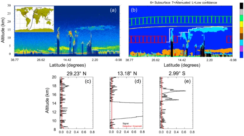
A detailed example of this technique is shown in Fig. 3, where the new 1064 nm feature detection algorithm evaluates a fairly typical blended cloud/aerosol scene for a nighttime granule. The 532 nm total attenuated backscatter is shown in Fig. 3a and the vertical feature mask (VFM) is shown in Fig. 3b. Superimposed on Fig. 3b are the frames correspond-ing to the two calibration transfer regions: V3, indicated by red boxes between 8 and 12 km, and V4, indicated using green boxes which track 2 km above the 400 K isentropic sur-face. Clearly, the V4 calibration transfer region is well above all features detected within the vertical feature mask.
deep convective cloud at 18◦N and a transparent cirrus cloud from 15◦N to 9.5◦S. The lower panels of Fig. 3 compare
the detection thresholds, T (z)(in red), to 1064 nm uncali-brated backscatter signals (in black) for three distinct features identified by the V3 L2 feature detection algorithm: clear-air (Fig. 3c), convective clouds (Fig. 3d), and cirrus clouds (Fig. 3e). The detection thresholds in these profiles are well selected to capture the clouds also detected by the V3 L2 al-gorithm in Fig. 3d and e. Meanwhile, the requirement that the signal exceedsT (z)for 1 km or more consecutive range bins prohibits false feature detections in the clear-air region (Fig. 3c). A more comprehensive validation of this 1064 nm feature detection technique is discussed in Sect. 4.3. 3.5 Derivation of attenuated scattering ratio and
scattering ratio uncertainty
The mathematical approach used to derive the 532 nm mean attenuated scatter ratios is fundamentally the same in both V3 and V4 (Powell et al., 2010). Attenuated scattering ratios and uncertainty are averaged for frames of data within the calibration transfer region. A “frame” is defined as 200 km along-track and 4 km vertical segments of data. Along-track, the 200 km resolution translates to 600 single shot (1/3 km native resolution) profiles. Those 1/3 km profiles that are considered invalid due to any errors or anomalies in the sig-nal are removed. Frames are excluded if they contain fea-tures identified by the 1064 nm feature detection algorithm summarized in Sect. 3.4.
Expanding Eq. (1), the nighttime attenuated scattering ra-tiosR0averaged for each frame are defined by
R0= 600 X
j=1 top X
i=base
βk,0measured(i, j )
βk,0 model(i, j ) . (9)
Here, the indexjis along track (horizontal direction) and in-dexiis from the base to top of the calibration transfer region in altitude (vertical direction). The nighttime attenuated scat-tering ratio uncertainties,1R0, averaged for each frame, is given by
1R0=R0 600 X j=1 top X
i=base
1Xk,0 measured(i, j ) X0k,model(i, j )
!2
+ 600 X
j=1
1Ck,night(j )
Ck,night(j ) !2
+ 600 X
j=1 top X
i=base
1βk,0 measured(i, j ) βk,0model(i, j )
!2
1/2
. (10)
This error quantifies the uncertainty associated with the mea-sured 532 nm parallel uncalibrated attenuated backscatter, the 532 nm molecular attenuated backscatter, and the 532 nm
nighttime parallel channel calibration coefficient, Ck,night. Given that the night-time calibration coefficient is reported only on a per profile basis within the data frame, its un-certainty contribution has to be accounted for differently than the backscatter components, which are averaged both horizontally and vertically. The derivation and scale of the 532 nm night-time calibration error term is described in more detail by Powell et al. (2009). A more detailed derivation of the 532 nm attenuated backscatter uncertainties can be found in Hostetler et al. (2006) and Liu et al. (2006).
The daytime averaged uncalibrated scattering ratios,Q0,
and uncertainties,1Q0, are computed using
Q0=
600 X j=1 top X i=base
Xk,0 measured(i, j )
βk,0 model(i, j ) , (11)
and
1Q0= 600 X j=1 top X i=base
1X0k,measured(i, j ) Xk,0 model(i, j )
!2 + 600 X j=1 top X i=base
1βk,0measured(i, j ) βk,0model(i, j )
!2
1/2
. (12)
BecauseQ0 uses uncalibrated data, accounting for the
con-tribution of the 532 nm nighttime calibration error is not re-quired.
3.6 Derivation of calibration coefficient and calibration coefficient uncertainty
The 532 nm calibration coefficients and their uncertainties for any given daytime granule are initially computed on a fixed elapsed time grid that spans from 0 s (referenced to the start of the daytime granule) to 3200 s with a resolution of 100 s. These coarse-resolution calibration coefficients are then linearly interpolated, based on time, and these interpo-lated values are applied to the 532 nm attenuated backscatter measurements at the 1/3 km native resolution.
Given the multi-day averaging needed to harvest the cali-bration data, as described in Sect. 3.3, time cannot be used, either elapsed or some other reference time, to aggregate day and night scattering ratios that span multiple orbits. The or-bital transition point from day to night (i.e., the day–night terminator), by which CALIPSO designates granules as ei-ther daytime or nighttime, changes throughout the aggrega-tion period. In order to properly account for this temporal drift, a reference latitude grid, independent of time, is built by mapping and interpolating the latitude of the daytime granule being calibrated onto the fixed elapsed time grid.
Figure 3.The(a)532 nm total attenuated backscatter and(b)vertical feature mask derived from the V3.01 lidar level 1 and level 2 data products for a nighttime orbital segment in 13 October 2010. For panel(b)the top of the features detected by the 1064 nm technique are identified by a solid white line, V3 calibration transfer regions are identified as red boxes, V4 calibration target regions are identified as green boxes, and the potential temperatures surface of 400 K is a solid yellow line. Profiles of uncalibrated 1064 nm signal with the applied detection threshold are shown in(c)–(e)for differing scenes contained in the orbit; clear, convective, and cirrus respectively.
grid cell(indexk)using
Ck,day(k)= D
Q0kE k D
R0kE k
= 1
N N P
n=1
Q0k,n
1
M M P
m=1
R0k,n
. (13)
N is the number of aggregated daytime scattering ratio frames and M is the number of night-time scattering ratio frames contained in each elapsed time grid cell.Ck,dayis sim-ply the ratio between the mean of the 532 nm un-calibrated daytime scattering ratios and the mean of the 532 nm cali-brated night-time scattering ratios.
The daytime calibration uncertainty estimate,1Ck,day, has contributions from both the 532 nm daytime and nighttime scattering ratio errors, as follows:
1Ck,day(k)=Ck,day(k) v u u t *
1Q0k
Q0k +
k +
* 1R0k
R0k +
k
. (14)
3.7 Accommodating missing data
Calibration coefficients derived from the day-to-night ratio of attenuated scattering ratios can only be calculated within those portions of an orbit in which both day and night ob-servations are acquired. Because of the illumination pat-terns in the polar regions during the solstice seasons, there
are no matching daytime and nighttime samples near the poles in summer and winter. This seasonally recurring lack of high latitude matching day and night data is accounted for by interpolating between the end points of the neigh-boring daytime and nighttime calibration coefficient curves. Where there are neither daytime and/or nighttime samples, the 532 nm daytime calibration coefficient and coefficient uncertainty curves are linearly interpolated as a function of orbital elapsed time anchored to the nearest neighboring 532 nm nighttime calibration. Figure 4 shows an example. In this orbit from July 2010, the day-to-night terminator occurs at∼60◦N, and thus no corresponding nighttime measure-ments are available over the final∼1100 s of the daytime granule. The impact of this interpolation on the accuracy of the calibration coefficients and uncertainty estimates is dis-cussed further in Sect. 4.1.
3.8 Calculating profiles of total attenuated backscatter coefficients
Figure 4. (a)532 nm daytime calibration and error for a 2 July 2010 daytime granule. The calibration and uncertainty for the high latitude segment (> 2050 s in the gray shaded region) are linearly interpolated between daytime calibration coefficients computed at a daytime granule elapsed time of 2050 s and the nighttime calibration coefficients at the beginning of the next nighttime orbit.(b)The orbit track (red line) for which the calibration coefficients shown in panel(a)were derived, and the adjoining night-side orbit track (blue line). That portion of the orbit which is interpolated because of the lack of any night-side measurements is indicated by the black dashed black line.
onboard calibration procedure described in detail in Hostetler et al. (2005), Hunt et al. (2009), and Powell et al. (2009). The calibration coefficients for the perpendicular channel are the product of the PGR and the parallel channel calibration coef-ficients; i.e.,
C⊥=PGR×Ck, (15)
(Powell et al., 2009). Given measured profiles ofPk(z)and
P⊥(z), the profiles of 532 nm total attenuated backscatter co-efficients,β0(z), reported in the CALIOP level 1 data product are derived using
β0(z)= r(z) 2
E
!
Pk(z) GkCk+
P⊥(z)
G⊥C⊥
. (16)
An identical procedure is followed for generating nighttime profiles ofβ0(z)(Kar et al., 2018).
3.9 Data latencies
Data latencies – i.e., the times between data acquisition and data product delivery – have also changed between V3 and V4. The CALIOP V3 standard data products are generated within 3 to 5 days from downlink, partially due to the V3 calibration approach but also because the analyses require a number of ancillary inputs that are not immediately available (Winker et al., 2009). The latency for the V4 standard prod-ucts is considerably longer. Because V4 uses the MERRA-2 meteorological data rather than the GMAO FPIT products, V4 standard products are typically not available until 6 to 10 weeks from downlink. However, the V3 expected prod-ucts continue to be available with 24–36 h from data acqui-sition (i.e.,∼12 h from data downlink). The expedited pro-cessing uses a faster (albeit less robust) calibration strategy,
as well as estimates for some of the other required informa-tion (e.g., platform attitude and ephemeris). The expedited products are tailored specifically for near-real-time process-ing applications, whereas the standard products are designed for rigorous scientific analyses.
4 Verification and validation 4.1 Mission level performance
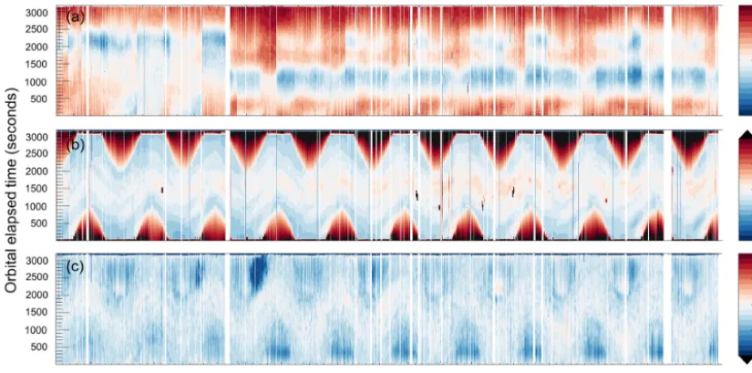
Performance of the 532 nm daytime calibration from 13 June 2006 to 31 December 2016 is shown in Fig. 5. Figure 5a shows the 532 nm daytime calibration coefficient anomalies while Fig. 5b shows the 532 nm daytime calibra-tion uncertainty anomalies, both of which are normalized to their respective time-series mean. The figure shows gaps in the data record occurring over the course of the mission, the reasons for which are described in more detail in Sect. 3.3. From the start of the mission to 31 December 2016 there have been 138 distinct events that required calibration restarts, with 71 of these due to planned maintenance of the lidar. The others were due to unscheduled events when either the in-strument was commanded to SAFE/OFF (leading to a period when no data was collected) or when data downlink issues caused delays that exceeded 24 h, and thus required a reboot of the calibration averaging, as described in Sect. 3.3. Also of note, the lidar switched from the primary laser to backup laser on 12 March 2009, resulting in a noticeable shift in the distributions of the calibration minimum between the two lasers.
Figure 5.Time series of(a)V4 532 nm daytime calibration coefficient anomalies,(b) calibration coefficient uncertainty anomalies, and (c)V4/V3 calibration ratio for 13 June 2006 to 31 December 2016 as functions of granule elapsed time. The calibration coefficients and uncertainties are extracted from the V4 and V3.x (3.01, 3.02, 3.30, and 3.40) L1 data files. The V4 532 nm daytime calibration coefficient and uncertainty anomalies are scaled to the means of the time series: 5.0619×10¹⁰km3sr J−1counts and 4.5088×10⁸km3sr J−1counts respectively.
in the distribution of the 532 nm calibration coefficient un-certainties in Fig. 5b. The saw tooth seasonal pattern of el-evated uncertainty, greater than 1.5 times above the normal-ized mean, directly corresponds to those areas of interpola-tion. Though the time series of the uncertainty is fairly stable throughout the mission, there are pockets at the mid-latitudes (∼1500 granule-elapsed seconds) in which there are local-ized spikes. These correspond to instances when there is a restart of the calibration with a greater contribution of signals from the SAA. As previously discussed, the multi-averaging window technique mitigates the impact of the influence of signal variability in the SAA on the calibration through sig-nificant cross-track averaging. However, in the case of a cali-bration restart the averaging window compresses and the im-pact of the SAA on the calibration uncertainties is amplified, though the overall mean is not.
The ratio between the V4 and V3 532 nm daytime cali-bration coefficients is shown in Fig. 5c. In general, the mid-latitude differences, corresponding to 1200–1800 granule-elapsed seconds, show differences in the range of ±5 %, with a global mean of 0.937 (6.3 %). This decrease in the calibration coefficient is expected, as there is an overall re-duction in the 532 nm nighttime calibration coefficients of approximately the same magnitude (Kar et al., 2018). The high-latitude reduction of the calibration ratio to 0.95 and less corresponds closely with the uncertainty in Fig. 5b. This reduction is also expected, because both the calibration and calibration uncertainty are interpolated to fit the neighboring night-time granules.
4.2 Zonal distributions of day and night attenuated scattering ratios
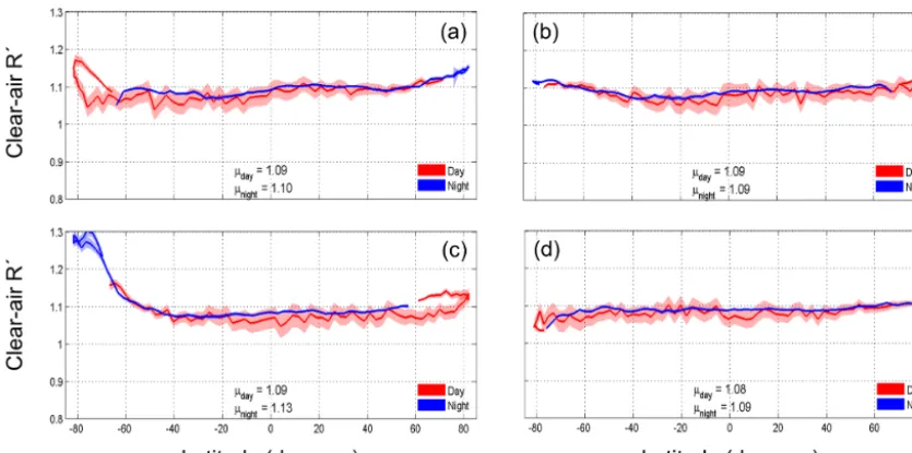
The performance of the new calibration algorithm can be evaluated by comparing zonal distributions of the day and night mean clear air attenuated scattering ratios in different altitude regimes. Comparisons of the calibration transfer re-gion are presented first. Given that the daytime calibration is scaled to the night-time, one should expect to see that the daytime and nighttime attenuated scattering ratios should tightly follow each other within this altitude band. Figure 6 confirms this expectation. The red and blue curves show, re-spectively, mean daytime and nighttime calibration coeffi-cients as a function of latitude, with the shaded areas around each curve delineating ±1 standard error about the mean. Comparisons are shown for each of the four seasons (Jan-uary, April, July, and October 2010). The SAA is excluded to minimize radiation-induced noise, and the L2 layer detec-tion results are used to guarantee that only clear-air regions are included.
From 60◦ north to south, for all four months, the mean
polar stratospheric features in the July nighttime data, and by unusually high noise levels introduced by the southern auro-ral radiation belt (Hunt et al., 2009) in the January daytime data.
The altitude region between 24 and 30 km is also exam-ined. These altitudes lie just above the top of the calibration transfer region used in the 532 nm daytime calibration, but below the 36–39 km region used by the 532 nm night-time calibration procedure. Thus, data within this region have not been used in either of the calibration procedures. Figure 7 shows the daytime–to–nighttime ratios of the clear air atten-uated scattering ratios measured in the 24–30 km region for both V3 (Fig. 7a) and V4 (Fig. 7b). The same months and data filtering procedures used in creating Fig. 6 are also used to construct Fig. 7. The V3 day-to-night ratios reveal high daytime biases of up to 20 % in the mid-latitudes and 25 % in the high-latitudes, with values above 1 consistently between ∼50◦S and∼60◦N. The V4 day-to-night ratios eliminate
the seasonal and latitudinal differences seen in V3. The V4 data are considerably more uniform and stable than the V3 data, with mean values of approximately one for all months and at all latitudes, confirming the ability of the V4 calibra-tion procedure to fully compensate for the high solar back-ground noise levels and thermal beam steering effects that are constantly present in CALIOP’s daytime measurements. 4.3 Probability of feature detection using 1064 nm
The V4 daytime calibration algorithm scans the uncalibrated 1064 nm measurements to ensure the presence of clear air down to the base of the calibration transfer regions. While the 532 nm channel is much more sensitive to the smaller aerosol particles that we expect to encounter most often in the stratosphere, the daytime calibration procedure does not require that we identify pristine air parcels. Instead, we need only identify and remove relatively robust, spatially varying, and temporally transient features – i.e., those layers that are not expected to persist uniformly across extended day–night cycles – and for this task the 1064 nm detection capabilities should be sufficient.
To establish the performance capabilities of our 1064 nm feature detection approach, 1 year of 532 nm daytime calibra-tions were regenerated using the more robust feature detec-tion and clearing provided by the 532 nm detecdetec-tion methods of the L2 algorithm. In creating this second set of calibration coefficients, the V4 5 km merged layer product was used to identify those V4 calibration transfer regions where layers of any type are reported in the L2 data products, and regions identified as being feature-contaminated were excluded from the subsequent calculations. Like the L1 detection scheme, the L2 algorithm uses fixed frames of data, but with a max-imum of 80 km rather than the 200 km horizontal averages used in L1. The L2 technique also employs multi-pass aver-aging (5, 20 and 80 km) and clearing to remove features de-tected at higher spatial resolutions prior to re-averaging and
searching for features at coarser resolutions. The L2 532 nm algorithm implementation is thus capable of identifying fea-tures at much finer spatial scales than the 1064 nm version of the search routine implemented in L1.
Figure 8 shows the ratios of these two sets of 532 nm cali-bration coefficients for the entirety of 2015, plotted as a func-tion of latitude. While some latitudinal deviafunc-tion is seen, the mean value (i.e., the black dashed line) varies by no more than±0.5 % about the expected value of 1, indicating that feature clearing using the 1064 nm data introduces essen-tially negligible perturbations to the derived calibration coef-ficients. The solid blue line in Fig. 8 shows the ratios formed when the V3 calibration coefficients are divided by the regen-erated V4 calibration coefficients. These values are compa-rable to those presented in Fig. 5c for the full mission V4/V3 comparison, and provide further evidence that the 1064 nm detection technique, if not ideal, is nevertheless both robust and reliable.
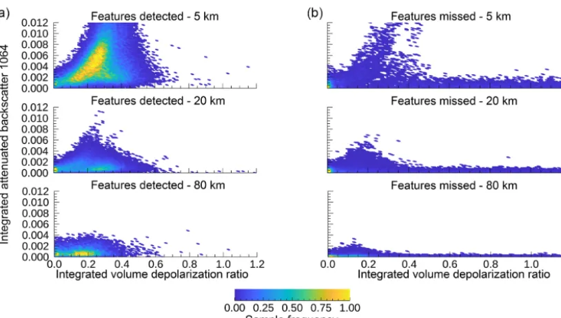
Figure 9 provides a more detailed examination of the fea-ture averaging and detection characteristics of the layers identified by the L2 532 nm feature detection algorithm and used in the re-calibration effort described in the previous paragraph. The plot is segregated by the effectiveness of the 1064 nm technique to detect features relative to the averaging required (i.e., 5, 20, or 80 km) to detect layers when using the 532 nm L2 detection scheme. The distributions of detected and undetected L2 features are plotted as a function of layer integrated volume depolarization (δv, x axis) and 1064 nm integrated attenuated backscatter (γ10640 , y axis). Figure 9 indicates that detection failures by the 1064 nm technique are likely due to the insensitivity of the 1064 nm signal to smaller particles. Those layers that are missed by the L1 1064 method, yet are detected by the L2 532 nm algorithm, most often have small IAB and low depolarization. It is also likely that the missed layers are being washed out at the 200 km 1064 nm detection resolution, and it would take a smaller spatial averaging window to isolate these features within the averaged signal profiles.
The preponderance of the 1064 nm detection failures is seen in the bottom left corners of the plots in the right-hand column of Fig. 9. These features, for which bothγ10640 and
Figure 6.Zonal clear-air attenuated scattering ratio (R); means (solid lines)±one standard error (shaded regions) for day and night in the calibration transfer regions for(a)January,(b)April,(c)July, and(d)October 2010. Global monthly means are given for both daytime (µday) and nighttime (µnight).
Figure 7.Day/night ratio of clear-air attenuated scattering ratio (R) mean±one standard error at 24–30 km for(a)V3 and(b)V4 for January, April, July, and October 2010. The SAA has been removed.
clouds (Pitts et al., 2009), values of this magnitude are highly unlikely for the bulk of the features that form in the strato-spheric regions searched during the 532 nm daytime calibra-tion procedure. Furthermore, 98 % of all layers in this study having γ10640 < 0.005 sr−1andδv> 0.7 were detected during the daytime when PSCs are not present and when the gen-eral susceptibility of the signal to noise at high altitudes is at its maximum. In both cases, these missed features (or false positives) are not being removed and are included in the 532 nm daytime calibration calculations. But as noted earlier, the overall impact of including these features is negligible.
Figure 8. Ratio of the V4 532 nm daytime calibrations derived based on 1064 nm detection technique (new L1 algorithm) to the calibrations derived by applying 532 nm feature clearing for 2015 in black. Red error-bars indicate that the mean calibration uncer-tainty. The blue line is the ratio of V4 to V3 daytime calibrations.
Figure 9.Distribution of layer integrated volume depolarization ratio and 1064 nm integrated attenuated backscatter for all features contained in the transfer regions used for calibration. In panel(a)are those instances when both the 532 and 1064 nm techniques have identified the prescience of a feature in the transfer regions, while in panel(b)are those instances when 532 nm found a layer while the 1064 nm did not. Distribution is also broken by the horizontal averaging used by the 532 nm V4 L2 feature detection, 5 km in the top row, 20 km in the middle row and 80 km in the bottom row.
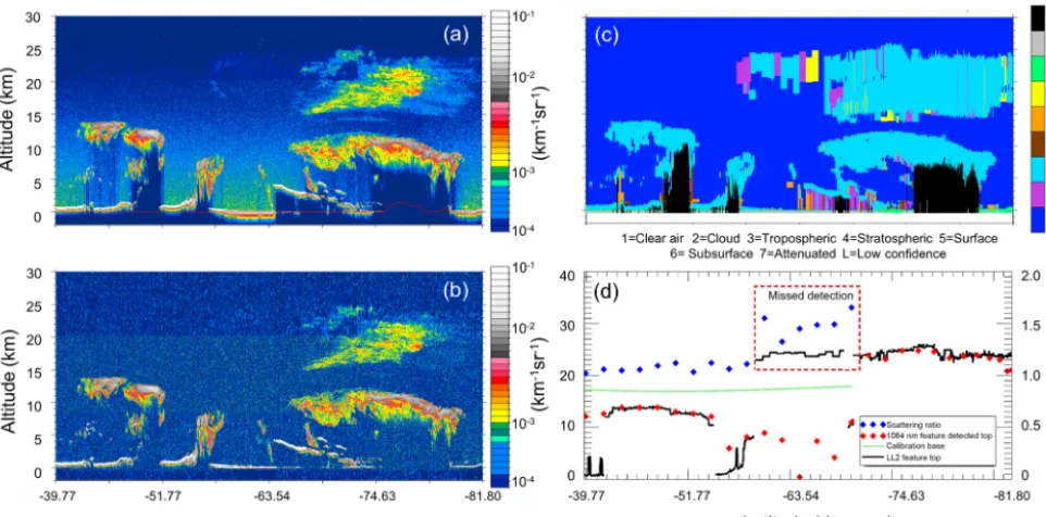
covering over half the along-track distance. Figure 10d com-pares L2 532 nm layer detections with the L1 1064 nm re-sults. The tops of the layers identified by the V4 L2 layer detection scheme are shown by solid black lines, while the tops of layers detected by the L1 1064 nm method are shown in red diamonds. Also show are the base altitudes of the cali-bration transfer region (green lines) and the 532 nm mean at-tenuated scattering ratios (blue diamonds) computed within those calibration transfer regions where no layer was de-tected by the L1 1064 nm algorithm.
The tops of the tropospheric clouds north of 57◦S are read-ily identified by the 1064 nm feature detection algorithm, but these lie below the base of the calibration transfer region. However, south of∼57◦S an extended PSC, with top alti-tudes at roughly 25 km, lies well within the calibration trans-fer region. The boxed area in Fig. 10d (dashed red lines) en-closes a region where the 1064 nm feature detection algo-rithm consistently failed to detect layers that are reported in the V4 VFM. When comparing the 1064 nm feature detection results to the 532 nm total attenuated backscatter (Fig. 10a) and 1064 nm attenuated backscatter (Fig. 10b), it is clear that 1064 nm feature detection is successful for strongly scattered features, but may have difficulty identifying the weakly scat-tering features. The 532 nm mean attenuated scatscat-tering ratios within the calibration transfer regions where layers were not detected by the 1064 nm feature detection algorithm are, on average, 50 % greater in this example than those in the
neigh-boring clear air regions (i.e.,∼1.5 vs.∼1.0 in the clear air regions). However, their ultimate impact on 532 nm daytime calibration is typically quite small due to extensive along-track and across-along-track averaging, as demonstrated in Fig. 8. And in this particular example, missed detections poleward of 67.5◦S do not contribute to calibration biases because the calibration coefficients at these latitudes are derived via in-terpolation, as described in Sect. 3.7.
4.4 Comparisons to HSRL measurements
From the beginning of the CALIPSO mission, the high spec-tral resolution lidar (HSRL) group at NASA-LaRC has ac-quired an extensive series of coincident airborne validation measurements. Following the release of the V3 L1 data set in April 2010, Rogers et al. (2011) conducted an in-depth analysis comparing HSRL 532 nm attenuated backscatter co-efficients measured along the CALIPSO orbit track to the 532 nm attenuated backscatter coefficients reported in the V3 CALIOP L1 data products. A major finding of this work showed that the CALIOP V3 daytime attenuated backscat-ter data was biased low with respect to the coincident HSRL data by 2.9 %±3.9 %.
Figure 10. (a)The 532 nm total attenuated backscatter;(b)1064 nm attenuated backscatter;(c)vertical feature mask; and(d)layer detection results for 15 July 2010 from 00:45 to 59:07. In panel(d), the uppermost layer top altitudes (km) detected by the 532 nm L2 algorithm are shown by black lines; layer top altitudes (km) detected by the 1064 nm L1 algorithm are shown by red diamonds; the base of the V4 calibration transfer region is shown by a green line; and blue diamonds show the 532 nm mean attenuated scattering ratios (unitless; right yaxis) in the calibration transfer regions where no layer was detected at 1064 nm.
field campaign (4–8 October 2011), and flights over the Azores (17 October 2012) and Bermuda (10–19 June 2014). In the process of reproducing the Rogers et al. (2011) V3 results, a bug was discovered in the code used to estimate the overlying two-way transmittance differences between the two sets of measurements (see Appendix A in Kar et al., 2018). Accounting for this error led to a small upward revi-sion of the daytime biases in the V3 data set, which we now estimate at 3.3 %±3.1 %. Running this same comparison us-ing the CALIOP V4 data and the larger coincident HSRL– CALIOP data set shows that the bias between the two sets of daytime measurements has now decreased to 1.0 %±3.5 %. The differences between the revised V3 analyses and the new V4 analyses are illustrated in Fig. 11. Further reduction of the CALIOP–HSRL bias in future analyses is unlikely. In doing the comparisons, the HSRL signals are corrected for known attenuations that occur between the CALIPSO satel-lite altitude and the HSRL aircraft altitude (e.g., molecu-lar and ozone attenuation). However, as explained in Kar et al. (2018), which focused on the nighttime comparisons be-tween CALIOP and HSRL, the HSRL measurements cannot be corrected for any attenuation due to undetected cloud or aerosol layers in this altitude regime (e.g., the background stratospheric aerosol layer). Failing to correct for an unde-tected optical depth of 0.005 would yield an attenuation bias of ∼1 %, a value that is essentially identical to our current estimate of the bias between CALIOP and HSRL.
Figure 11.Bias of the daytime 532 nm attenuated backscatter mea-sured between HSRL and CALIPSO for several over-flight cam-paigns between 2006 and 2014 broken by season and latitudes. The comparisons used both V3 (solid diamonds) and V4 (open circles) L1 data. Each point represents the mean and uncertainty of the HSRL-CALIPSO difference for each of the 62 flights conducted.
5 Concluding remarks
com-prehensive estimates of calibration uncertainties. The new V4 algorithm keeps the underlying approach that was used in V3, wherein the 532 nm daytime calibration coefficients are scaled relative to the 532 nm nighttime coefficients, which are calculated using the highly reliable high-altitude nor-malization technique. The simplified V4 calibration archi-tecture reduces software coupling and increases cohesion by eliminating the need for multi-pass product generation cy-cle, which in turn enables a more direct computation of the calibration coefficients and their uncertainties. The V4 cal-ibration performance meets pre-defined expectations estab-lished from internal science impact testing, and fully satis-fies numerous day–night consistency metrics. Elevating the calibration transfer region, coupled with a revised feature detection scheme that uses the uncalibrated 1064 nm mea-surement, has greatly increased the probability that the at-tenuated scattering ratios used in deriving the calibration co-efficients are computed within clear air regions and largely eliminated the diurnal aerosol loading artifacts seen in V3. Independent validation using collocated high spectral resolu-tion lidar measurements shows a demonstrable improvement between CALIOP V3 and V4 daytime calibration, with the mean daytime bias between the two sets of measurements being reduced from 3 % to approximately 1 %.
Data availability. The following CALIPSO data
prod-ucts were used in this study: the V3.01 CALIPSO level 1 profile product (Vaughan et al., 2018; NASA Lang-ley Research Center Atmospheric Science Data Center; https://doi.org/10.5067/CALIOP/CALIPSO/CAL_LID_L1-ValStage1-V3-01_L1B-003.01; last access 1 May 2018); the V3.02 CALIPSO level 1 profile product (Vaughan et al., 2018; NASA Langley Research Center Atmospheric Science Data Center; https://doi.org/10.5067/CALIOP/CALIPSO/CAL_LID_L1-ValStage1-V3-02_L1B-003.02; last access 1 May 2018); the V3.30 CALIPSO level 1 profile product (Vaughan et al., 2018; NASA Langley Research Center Atmospheric Science Data Center; https://doi.org/10.5067/CALIOP/CALIPSO/CAL_LID_L1-ValStage1-V3-30_L1B-003.30; last access 1 May 2018); the V3.40 CALIPSO level 1 profile product (Vaughan et al., 2018; NASA Langley Research Center Atmospheric Science Data Center; https://doi.org/10.5067/CALIOP/CALIPSO/CAL_LID_L1-ValStage1-V3-40; last access 1 May 2018); the V4.10 CALIPSO level 1 profile product (Vaughan et al., 2018; NASA Lan-gley Research Center Atmospheric Science Data Center; https://doi.org/10.5067/CALIOP/CALIPSO/LID_L1-Standard-V4-10; last access 1 May 2018); the V3.01 CALIPSO level 2 vertical feature mask product (Vaughan et al., 2018; NASA Langley Research Center Atmospheric Science Data Center; https://doi.org/10.5067/CALIOP/CALIPSO/CAL_LID_L2-ValStage1-V3-01_L2-003.01; last access 1 May 2018); and the V4.10 CALIPSO level 2 5 km merged layer product (Vaughan et al., 2018; NASA Langley Research Center Atmospheric Science Data Center; https://doi.org/10.5067/CALIOP/CALIPSO/LID_L2-05kmMLay-Standard-V4-10; last access 1 May 2018). The CALIPSO level 1 and level 2 data products are also available
from the AERIS/ICARE Data and Services Center. HSRL data are available by request from the authors (Mark Vaughan at [email protected]) or from the NASA-Langley HSRL team (John Hair at [email protected]).
Author contributions. All co-authors have contributed to the paper, and the order in which they are listed is primary author’s best esti-mate as to their level of contribution.
Competing interests. The authors declare that they have no conflict of interest.
Special issue statement. This article is part of the special issue “CALIPSO version 4 algorithms and data products”. It is not associated with a conference.
Edited by: James Campbell
Reviewed by: Zhien Wang and J. Yorks
References
Chand, D., Wood, R., Anderson, T. L., Satheesh, S. K., and Charlson, R. J.: Satellite-derived direct radiative effect of aerosols dependent on cloud cover, Nat. Geosci., 2, 181–184, https://doi.org/10.1038/ngeo437, 2009.
Forbes, R. M. and Ahlgrimm, M.: On the representation of high-latitude boundary layer mixed-phase cloud in the ECMWF global model, Mon. Weather Rev., 142, 3425–3445, https://doi.org/10.1175/MWR-D-13-00325.1, 2014.
Gelaro, R, McCarty, W., Suárez, M. J., Todling, R., Molod, A., Takacs, L., Randles, C. A., Darmenov, A., Bosilovich, M. G., Re-ichle, R., Wargan, K., Coy, L., Cullather, R., Draper, C., Akella, S., Buchard, V., Conaty, A., da Silva, A. M., Gu, W., Kim, G., Koster, R., Lucchesi, R., Merkova, D., Nielsen, J. E., Partyka, G., Pawson, S., Putman, W., Rienecker, M., Schubert, S. D., Sienkiewicz, M., and Zhao, B.: The Modern-Era Retrospective Analysis for Research and Applications, Version 2 (MERRA-2), J. Climate, 30, 5419–5454, https://doi.org/10.1175/JCLI-D-16-0758.1, 2017.
Gettelman, A. and Wang, T.: Structural diagnostics of the tropopause inversion layer and its evolution, J. Geophys. Res.-Atmos., 120, 46–62, https://doi.org/10.1002/2014JD021846, 2015.
Hoskins, B.: Towards a PV-θView of the General Circulation, Tel-lus, 43, 27–35, https://doi.org/10.1034/j.1600-0889.1991.t01-3-00005.x, 1991.
Hostetler, C. A., Liu, Z., Reagan, J. A., Vaughan, M. A., Winker, D.M., Osborn, M. T., Hunt, W. H., Powell, K. A., and Trepte, C. R.: CALIPSO algorithm theoretical basis document, PC-SCI-201, available at: https://www-calipso.larc.nasa.gov/resources/ project_documentation.php (last access: 25 June 2018), 2006. Hu, Y., Winker, D., Vaughan, M., Lin B., Omar, A., Trepte,
and Holz, R.: CALIPSO/CALIOP Cloud Phase Discrimi-nation Algorithm, J. Atmos. Ocean. Tech., 26, 2293–2309, https://doi.org/10.1175/2009JTECHA1280.1, 2009.
Hunt, W. H., Winker, D. M., Vaughan, M. A., Powell, K. A., Lucker, P. L., and Weimer, C.: CALIPSO Lidar Description and Per-formance Assessment, J. Atmos. Ocean. Tech., 26, 1214–1228, https://doi.org/10.1175/2009JTECHA1223.1, 2009.
Kar, J., Vaughan, M. A., Lee, K.-P., Tackett, J. L., Avery, M. A., Garnier, A., Getzewich, B. J., Hunt, W. H., Josset, D., Liu, Z., Lucker, P. L., Magill, B., Omar, A. H., Pelon, J., Rogers, R. R., Toth, T. D., Trepte, C. R., Vernier, J.-P., Winker, D. M., and Young, S. A.: CALIPSO lidar calibration at 532 nm: ver-sion 4 nighttime algorithm, Atmos. Meas. Tech., 11, 1459–1479, https://doi.org/10.5194/amt-11-1459-2018, 2018.
Kim, M.-H., Omar, A. H., Tackett, J. L., Vaughan, M. A., Winker, D. M., Trepte, C. R., Hu, Y., Liu, Z., Poole, L. R., Pitts, M. C., Kar, J., and Magill, B. E.: The CALIPSO version 4 automated aerosol classification and lidar ratio selection algorithm, At-mos. Meas. Tech., 11, 6107–6135, https://doi.org/10.5194/amt-11-6107-2018, 2018.
Liu, Z., Hunt, W., Vaughan, M., Hostetler, C., McGill, M., Powell, K., Winker, D., and Hu, Y.: Estimating Random Errors Due to Shot Noise in Backscatter Lidar Observations, Appl. Opt., 45, 4437–4447, https://doi.org/10.1364/AO.45.004437, 2006. Liu, Z., Vaughan, M. A., Winker, D. M., Kittaka, C., Kuehn,
R. E., Getzewich, B. J., Trepte, C. R., and Hostetler, C. A.: The CALIPSO Lidar Cloud and Aerosol Dis-crimination: Version 2 Algorithm and Initial Assessment of Performance, J. Atmos. Ocean. Tech., 26, 1198–1213, https://doi.org/10.1175/2009JTECHA1229.1, 2009.
Liu, Z., Kar, J., Zeng, S., Tackett, J., Vaughan, M., Avery, M., Pelon, J., Getzewich, B., Lee, K.-P., Magill, B., Omar, A., Lucker, P., Trepte, C., and Winker, D.: Discriminating Between Clouds and Aerosols in the CALIOP Version 4.1 Data Products, Atmos. Meas. Tech. Discuss., https://doi.org/10.5194/amt-2018-190, in review, 2018.
Manney, G. L. and Hegglin, M. I.: Seasonal and Regional Variations of Long-Term Changes in Upper-Tropospheric Jets from Reanal-yses, J. Climate, 31, 423–448, https://doi.org/10.1175/JCLI-D-17-0303.1, 2018.
Omar, A., Winker, D., Kittaka, C., Vaughan, M., Liu, Z., Hu, Y, Trepte, C., Rogers, R., Ferrare, R., Kuehn, R., and Hostetler, C.: The CALIPSO Automated Aerosol Classification and Lidar Ra-tio SelecRa-tion Algorithm, J. Atmos. Ocean. Tech., 26, 1994–2014, https://doi.org/10.1175/2009JTECHA1231.1, 2009.
Pitts, M. C., Poole, L. R., and Thomason, L. W.: CALIPSO polar stratospheric cloud observations: second-generation detection al-gorithm and composition discrimination, Atmos. Chem. Phys., 9, 7577–7589, https://doi.org/10.5194/acp-9-7577-2009, 2009. Powell, K. A., Vaughan, M. A., Kuehn, R., Hunt, W. H., and Lee,
K.-P.: Revised Calibration Strategy for the CALIOP 532-nm Channel: Part II – Daytime, in: Reviewed and Revised Papers Presented at the 24th International Laser Radar Conference, 23– 27 June, 2008, Boulder, CO, USA, 1177–1180, 2008.
Powell, K. A., Hostetler, C. A., Liu, Z., Vaughan, M. A., Kuehn, R. E., Hunt, W. A., Lee, K.-P., Trepte, C. R, Rogers, R. R, Young, S. A., and Winker, D. M.: CALIPSO Lidar Calibration Algo-rithms: Part I – Nighttime 532 nm Parallel Channel and 532 nm
Perpendicular Channel, J. Atmos. Ocean. Tech., 26, 2015–2033, https://doi.org/10.1175/2009JTECHA1242.1, 2009.
Powell, K. A., Vaughan, M. A., Rogers, R. R., Kuehn, R. E., Hunt, W. H., Lee, K.–P., and Murray, T. D.: The CALIOP 532-nm Channel Daytime Calibration: Version 3 Algorithm, in: 25th In-ternational Laser Radar Conference, 5–9 July, 2010, St. Peters-burg, Russia, 1177–1180, ISBN: 978-0-615-21489-4, 2010. Reichler, T., Dameris, M., and Sausen, R.: Determining the
tropopause height from gridded data, Geophys. Res. Lett., 30, 2042, https://doi.org/10.1029/2003GL018240, 2003.
Rogers, R. R., Hostetler, C. A., Hair, J. W., Ferrare, R. A., Liu, Z., Obland, M. D., Harper, D. B., Cook, A. L., Powell, K. A., Vaughan, M. A., and Winker, D. M.: Assessment of the CALIPSO Lidar 532 nm attenuated backscatter calibration using the NASA LaRC airborne High Spectral Resolution Lidar, At-mos. Chem. Phys., 11, 1295–1311, https://doi.org/10.5194/acp-11-1295-2011, 2011.
Russell, P. B., Swissler, T. J., and McCormick, M. P.: Methodology for error analysis and simulation of lidar aerosol measurements, Appl. Opt., 18, 3783–3797, 1979.
Sassen, K. and Hsueh, C.-Y.: Contrail properties derived from high-resolution polarization lidar studies during SUCCESS, Geophys. Res. Lett., 25, 1165–1168, https://doi.org/10.1029/97GL03503, 1998.
Stephens, G., Winker, D., Pelon, J., Trepte, C., Vane, D., Yuhas, C., L’Ecuyer, T., and Lebsock, M.: CloudSat and CALIPSO within the A-Train: Ten years of actively observ-ing the Earth system, B. Am. Meteorol. Soc., 99, 583–603, https://doi.org/10.1175/BAMS-D-16-0324.1, 2018.
Tan, I., Storelvmo, T., and Zelinka, M. D.: Observational constraints on mixed-phase clouds imply higher climate sensitivity, Science, 352, 224–227, https://doi.org/10.1126/science.aad5300, 2016. Vaughan, M. A., Winker, D. M., and Powell, K. A.: CALIOP
Algorithm Theoretical Basis Document, Part 2: Feature De-tection and Layer Properties Algorithms, PC-SCI-202.01, available at: https://www-calipso.larc.nasa.gov/resources/ project_documentation.php, (last access: 25 June 2018), 2005. Vaughan, M., Powell, K., Kuehn, R., Young, S., Winker, D.,
Hostetler, C., Hunt, W., Liu, Z., McGill, M., and Getzewich, B.: Fully Automated Detection of Cloud and Aerosol Layers in the CALIPSO Lidar Measurements, J. Atmos. Ocean. Tech., 26, 2034–2050, https://doi.org/10.1175/2009JTECHA1228.1, 2009. Vaughan, M. A., Liu, Z., McGill, M. J., Hu, Y., and Obland, M. D.: On the spectral dependence of backscatter from cirrus clouds: Assessing CALIOP’s 1064 nm calibration assumptions using cloud physics lidar measurements, J. Geophys. Res., 115, D14206, https://doi.org/10.1029/2009JD013086, 2010. Vaughan, M., Pitts, M., Trepte, C., Winker, D., Detweiler, P.,
Gar-nier, A., Getzewich, B., Hunt, W., Lambeth, J., Lee, K.-P., Lucker, P., Murray, T., Rodier, S., Tremas, T., Bazureau, A., and Pelon, J.: Cloud-Aerosol LIDAR Infrared Pathfinder Satellite Observations (CALIPSO) data management system data prod-ucts catalog, Release 4.40, NASA Langley Research Center Doc-ument PC-SCI-503, 173 pp., available at: https://www-calipso. larc.nasa.gov/products/CALIPSO_DPC_Rev4x40.pdf, last ac-cess: 25 June 2018.
layer from CALIPSO lidar observations, J. Geophys. Res., 114, D00H10, https://doi.org/10.1029/2009JD011946, 2009. Vernier, J.-P., Thomason, L. W., and Kar J.: CALIPSO detection
of an Asian tropopause aerosol layer, Geophys. Res. Lett., 38, L07804, https://doi.org/10.1029/2010GL046614, 2011. Winker, D. M., Vaughan, M. A., Omar, A. H., Hu, Y.,
Pow-ell, K. A., Liu, Z., Hunt, W. H., and Young, S. A.: Overview of the CALIPSO Mission and CALIOP Data Pro-cessing Algorithms, J. Atmos. Ocean. Tech., 26, 2310–2323, https://doi.org/10.1175/2009JTECHA1281.1, 2009.