GLOBAL JOURNAL OF ADVANCED ENGINEERING TECHNOLOGIES AND
SCIENCES
A REDUCED SPACE COMBINED WITH TABU SEARCH FOR SOLVING THE
CHANNEL ALLOCATION PROBLEM
Jayrani Cheeneebash*, Harry C S Rughooputh and Jose A Lozzano
*Department of Mathematics, Faculty of Science, University of Mauritius, Reduit, Mauritius
DOI
: 10.5281/zenodo.1163157
ABSTRACT
With the rapid growth of mobile communications, solving the channel assignment problem has now become a new challenge in research. In this paper, we present an efficient technique for solving the Channel Assignment Problem (CAP). We first map a given CAP, P, to a smaller subset Pof cells of the network, which actually reduces the search space. This reduction is done using a multi-colouring method. Then the tabu search algorithm is applied to solve the new problem P. This method reduces the computing time drastically. The latter is then used to solve the original problem by using a modified forced assignment with rearrangement (FAR) operation. The proposed method has been tested on well known benchmark problems. Optimal solutions have been obtained with zero blocked calls for all the cases with improved computation time. Furthermore, there are many unused frequencies which can be used for changes in demands.
KEYWORDS: Channel Allocation Problem, FAR, Tabu Search.
INTRODUCTION
Mobile communications are evolving rapidly with the progress of wireless communications and mobile computing. However, the frequency bandwidth is limited and an efficient use of channel frequencies becomes more and more important. The bandwidth spectrum is divided into a number of channels depending on service requirements. To satisfy high demand of mobile users, channels have to be assigned and re-used to minimize communication interference, thus increasing traffic carrying capacity. This is known as the channel assignment problem (CAP). In other words, the CAP is considered to be the generalised graph colouring problem, which is a well known NP-complete problem [13]. In this paper we assume a cellular network system where the demands of the cells are known a priori, and the channels are to be allocated to the cells statistically to cater sessions that are basically connection oriented. Here, the major aim is to reuse channels in cells while avoiding interference. A channel can be used by multiple base stations if the minimum distance at which two signals of the same frequency do not interfere.
The paper is structured as follows: section 2 gives the mathematical formulation of the CAP, section 3 presents the tabu search algorithm, section 4 shows how the CAP is reduced and section 5 explains the FAR algorithm. Simulation results are discussed in section 6 and finally
we draw some concluding remarks.
MATEMATICAL FORMULATION OF CAP
The CAP in cellular networks is an NP-complete problem [13]. It has been modelled as an optimization problem with binary solutions. The problem is characterized by a number of cells and a number of channels n and f respectively. It must fulfill the following three constraints [10]:
1. The Co-Channel Constraint (CCC): The same channel cannot be assigned to a pair of cells within a specified distance simultaneously.
2. The Adjacent Channel Constraint (ACC): Adjacent Channels cannot be assigned to adjacent cells simultaneously.
3. The Co-site Constraint (CSC): The distance between any pair of channels used in the same cell must be larger than a specified distance.
In 1982, Gamst and Rave [10] defined the general form of the CAP in an arbitrary inhomogeneous cellular network. In their definition, the compatibility constraints in an n - cell network are described by an n × n symmetric matrix called the compatibility matrix C = [ci j]. Each non-diagonal element ci j in C represents the minimum
separation distance in the frequency domain between a frequency assigned to a cell i and one assigned to cell j. If
ci j = 0, it means that a channel assigned to cell i can be reused to cell j; cii = s means the co-site channel interference
constraint is s channels. ci j = 1 means that the adjacent channel interference constraint is one channel. The channel
requirements are described by an n-element vector which is called the demand vector D. Each element di in D
represents the number of frequencies to be assigned to cell i. The solution of the CAP is represented by a matrix
F. Each element of the matrix is defined according to the following expression:
otherwise 0
cell to assigned s
channel if
1 ji i
aij
.
Let the frequencies be represented by positive integers 1, 2, 3,..., f where f is a maximum allocation of the spectrum bandwidth. The mathematical model can be represented as follows [21, 24]:
1. n: Number of cells in the network.
2. di: Number of frequencies required in cell i (1 ≤ i ≤ n) in order to satisfy channel demand.
3. C: Compatibility matrix, C = (cij) denotes the frequency
separation required between cell i and cell j. 4. fik: Channel is assigned to kth call in cell i.
Therefore the objective of CAP is
, min
,k ik i
f subject to fik fjr ciji,j,kr.
The channel assignment problem in the cellular network is to find a conflict free assignment with the minimum number of total frequencies, where C and D are given, in other words one tries to find the minimum of
. max
,k ik i
f
Given the above constraints, the CAP can be represented by means of a graph G, where the k-th call to cell i is
represented as a node
ik and the nodes
ikand
jr are connected by an edge with weightc
ijifc
ij
0
. Then, the channels are assigned to the nodes of the CAP graph in a specific order and a node will be assigned the channel corresponding to the smallest integer that will satisfy the frequency separation constraints with all the previously assigned nodes. Thus one can conclude that the ordering of the nodes is a key factor on the required bandwidth. Let us assume that there exists m nodes in the CAP graph, where m is defined as the total demand, in other words
n i
i d m
1
. Therefore the nodes can be ordered in
m
!ways and finding the optimal ordering is an exhaustivetask. In this paper we have used a tabu search adapted from [12] which is an efficient algorithm for solving permutation problems.
TABU SEARCH APPROACH
and neighborhood that has been used in the tabu search. Denoting p to be a random ordering of the n cells. The Insert-Move(pj; i) function consists of deleting pj from its current position j to be inserted in position i. Thus one
gets the following ordering
p
as shown in (1) . for ) ,..., , , ,..., , ,..., , for ) ,..., , ,..., , , ,..., ( 1 1 1 1 1 1 1 1 j i p p p p p p p j i p p p p p p p p n i j i j j n j j i j i (1)
Pairwise exchanges or moves are frequently used as one of the ways to define neighbourhoods in permutation problems; identifying moves that lead from one sequence to the next. The neighbourhood N comprises all permutations resulting from executing general insertion moves and is defined as
(3) ,..., 1 , 1 ,..., 2 , 1 and (2) ,..., 1 for ), , ( Move -Insert : n j j i n j i p p N j
We define a first strategy, that scans the list of cells (in the order given by the current permutation) in search for the first cell (pf) whose movement results in a strictly positive move value. The move selected by the
first
strategyis then Insert-Move(pf ; i*_), where i*is the position that gives the best move value. The local search is based on
choosing the best insertion associated with a given cell. The tabu search procedure starts by generating a random procedure p, and it alternates between an intensification and a diversification phase. The main aim of the search intensification is to explore more thoroughly the portions of the search space that seem “promising” in order to ensure that the best solutions in these areas are indeed found.
Intensification is based on some intermediate term memory, such as a recency memory, in which one records the number of consecutive iterations that various solutions components have been present in the current solution without interruption. The intensification phase starts by a random selection of a cell. The probability of selecting a cell j is proportional to some weight wj. For our problem, we assign higher weights to those cells having a higher
demand. The weight is given as
n j j j j d d w 1 .The move Insert-Move(pj,i)N jwith the largest move value is selected and it becomes the tabu-active for
TabuTenure iterations. The number of times that cell j has been chosen to be moved is accumulated in the value
freq( j). This frequency information is used for diversification purposes. The intensification phase is terminated after a maximum of a predefined number of iterations is executed without improvement. Before ending this phase, the first(N) procedure is applied to the best solution which is denoted by pˆ.
Diversification phase is an algorithmic mechanism that forces the search into previously unexplored areas of the search space. It is usually based on some form of long term memory of a sector and in our case it is the frequency memory in which one records the total number of iterations that various solution components have been present in the current solution. At each iteration of the diversification phase, a sector is selected randomly and the probability of selecting sector j is inversely proportional to the frequency count freq( j). The chosen sector is placed in the best position, as determined by the move values associated with the insert moves in Nj. This
procedure is repeated for a maximum number of iterations.
CONSTRUCTION OF THE REDUCED SPACE
In this section we describe how the CAP graph G is reduced into a smaller space and we use tabu search to find an optimal solution which is then considered to solve the original CAP problem. Our aim is to find out independent sets of cells by the multicolouring method. Let us assume that G denotes the adjacency graph of the n× n matrix
Ci, j=1,…,n and has a vertex set V(G) and edge set E(G). We say that (i,j)E(G)(i; j) if and only if cij 0. A
node or vertex i is said to be connected to node j if jadj(i) whereadj(i)
j(i,j)
E(G). The degree of vertex i is the size of its adjacency set (adj(i)). A proper colouring of G is an assignment of colours to vertices such that no two end points of any edge share the same colour. A set S is said to be an independent set of V(G). )} ( ) , ( or ) ( ) , ( then
if iS i j EG j i EG jS Thus the elements in S cannot be connected among
the graph in the natural order and assigns thesmallest positive admissible colour to each node i visited.Here, an admissible colour is a colour not already assigned to any neighbour of node i.
——————————————————————–
Greedy Multi Colouring Algorithm
——————————————————————– Set Colour(i) = 0; i = ,…, N
for i = 1 : N
Colour(i) = min{l > 0|j ≠ Colour( j), for all jadj(i)}
end
The end result of the algorithm is that each node i will be assigned the colour Colour(i). The algorithm stops until all the nodes have been visited.
After having obtained the independent sets, we then form the reduced compatibility matrix. We then apply the tabu search algorithm to assign the frequencies to the reduced space. We shall illustrate our method by means of an example, problem 3 in Table 4 from the Philadelphia benchmark problems. The CAP, P, has been formulated on a 21-cell system whose compatibility matrix C and the demand vector D1 is shown in Tables 1 and Tables 3 respectively. Denoting S (i) to be the set of all cells that are not connected, we illustrate an example for the problem described above. Suppose after applying the multi-colouring algorithm, we obtain the following: S (1) = {5,7,21}, S (2) = {10.19}, S (3) = {9,12,14}, S (4) = {8,13,18}, S (5) = {3,15}, S (6) = {6,20}, S (7) = {1,17}, S (8) = {2,11}and S (9) = {4,16}. From the set S we now construct the compatibility matrix Cc(i,j) as follows.
We get c(1,2)1 being the maximum among all the ci,j where i S(1) {8,21}andjS(2){10,15}. We thus obtain the elements of C as shown in Table 2. In this example we can find that the demand for the elements in S (1) are 12, 30 and 25. The maximum demand is 30. Similarly the demand for S (2) = 40, S (3) = 45, S (4) = 30, S (5) 25, S (6) = 25, S (7) = 15, S (8) = 40, and S (9) = 15. Thus the modified demand vector
). 15 , 40 , 15 , 25 , 25 , 30 , 45 , 40 , 30 (
D The new problem Pis represented by the following components:
1. a set S{S(1),...,S(z)},(1iz) of z distinct nodes, where z is the number of S (i) subsets. 2. a demand vector D(d1,...,dz).
3. a compatibility matrix Cc(i,j).
4. a frequency assignment matrix F.
5. a set of frequency separation constraints specified by the frequency separation matrix fik fjl for all
i, j, k, l (except for i = j and k = l).
Once P is constructed as above, the aim is to find an assignment F for this P. We describe how the CAP is solved using the tabu search algorithm. First, we define the blocked calls; they are the number of calls without an allocated frequency and the lower the number of blocked calls the better solution. Our aim is to minimize the number of blocked calls. We start our simulation by a random ordering or permutation of the cells and the tabu search is applied as shown in the algorithm below.
——————————————————————– Procedure to apply the algorithm
——————————————————————– Generate a random permutation order of the
the elements of S . for j = 1 to maxiter
Apply intensification phase. Apply first(N).
Apply diversification phase. Calculate solution matrix F. [calculate number of blocked calls]. If number of blocked calls = 0, break loop. Calculate maxglob iterations > 5
end j
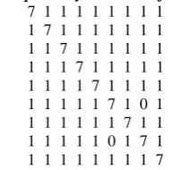
Table 1: Compatibility Matrix for Problem 3
7 1 1 0 0 1 1 1 1 0 0 0 0 1 1 1 0 0 0 0 0 1 7 1 1 0 0 1 1 1 1 0 0 0 0 1 1 1 0 0 0 0 1 1 7 1 1 0 0 1 1 1 1 0 0 0 0 1 1 1 0 0 0 0 1 1 7 1 0 0 0 1 1 1 1 0 0 0 0 1 1 0 0 0 0 0 1 1 7 0 0 0 0 1 1 1 0 0 0 0 0 1 0 0 0 1 0 0 0 0 7 1 1 0 0 0 0 1 1 1 0 0 0 0 0 0 1 1 0 0 0 1 7 1 1 0 0 0 1 1 1 1 0 0 1 0 0 1 1 1 0 0 1 1 7 1 1 0 0 0 1 1 1 1 0 1 1 0 1 1 1 1 0 0 1 1 7 1 1 0 0 0 1 1 1 1 1 1 1 0 1 1 1 1 0 0 1 1 7 1 1 0 0 0 1 1 1 0 1 1 0 0 1 1 1 0 0 0 1 1 7 1 0 0 0 0 1 1 0 0 1 0 0 0 1 1 0 0 0 0 1 1 7 0 0 0 0 0 1 0 0 0 0 0 0 0 0 1 1 0 0 0 0 0 7 1 1 0 0 0 0 0 0 1 0 0 0 0 1 1 1 0 0 0 0 1 7 1 1 0 0 1 0 0
1 1 0 0 0 1 1 1 1 0 0 0 1 1 7 1 1 0 1 1 0 1 1 1 0 0 0 1 1 1 1 0 0 0 1 1 7 1 1 1 1 1 0 1 1 1 0 0 0 1 1 1 1 0 0 0 1 1 7 1 1 1 1 0 0 1 1 1 0 0 0 1 1 1 1 0 0 0 1 1 7 0 1 1 0 0 0 0 0 0 1 1 1 0 0 0 0 1 1 1 1 0 7 1 1 0 0 0 0 0 0 0 1 1 1 0 0 0 0 1 1 1 1 1 7 1 0 0 0 0 0 0 0 0 1 1 1 0 0 0 0 1 1 1 1 1 7
Table 2: Compatibility Matrix Pfor Problem 3.
7 1 1 1 1 1 1 1 1 1 7 1 1 1 1 1 1 1 1 1 7 1 1 1 1 1 1 1 1 1 7 1 1 1 1 1 1 1 1 1 7 1 1 1 1 1 1 1 1 1 7 1 0 1 1 1 1 1 1 1 7 1 1 1 1 1 1 1 0 1 7 1 1 1 1 1 1 1 1 1 7
Now we need to apply the FAR algorithm to solve the original CAP problem with a view that our objective is to minimise the number of blocked calls. The assignment F may or may not be admissible depending on the available bandwidth. To derive the required channels for the CAP, we have adapted the method found in [11]. They considered the following two cases:
1. An assignment F is admissible: For this case, an admissible frequency for the original problem can be derived using F and the following result [11]:
Given the CAP problem P and the bandwidth, if the frequency assignments F for P are admissible, an admissible frequency can be derived from F. To get an assignment F, all the cells in S (i); 1 ≤ i ≤ z are assigned the same set of channels. This assignment must satisfy the interference constraints because in P, c(i,j) is the maximum among all the terms ci j’s in C, where i iS(i)and jS(j). This assignment must also satisfy the
demand vector D = di, since we choose the maximum among all those cells found in S(i). When applying this
procedure, one also gets some redundant frequencies. Suppose if cell i has been assigned di channels where the demand for that cell was di and did(i), then ri (didi)number of frequencies remains unused or redundant
in cell i.
2. Assignment F is not admissible: For this case the requirements forP. Let us assume F that satisfies the demand vector D(di)i ) instead of D, where didi for some i. If we assign all the cells in S (i) the same set of channels to the cells in S (i), there may be some blocked calls in some cells and redundant calls in some other cells. We denote the blocked calls and redundant frequencies as follows:
BL = (bi) and R = (r j), respectively, where bi di diif didi and 0 otherwise, and
j j j j
j d d d d
r ( ), if and 0 otherwise. We use these redundant frequencies in R and other available free channels to assign the blocked calls by using the FAR approach described in [14].
We give a brief description of the modified FAR algorithm. Let bi be an unassigned requirement and Q be the set
any conflict to the set Q. The modified FAR tries to assign a frequency in L (where L is the given list of available frequencies) to satisfy the requirement bi with minimum change or perturbation on the present assignment Q. The
main aim of modified FAR is to identify a minimal subset bi’s of Q, where each requirement can be reassigned
simultaneously with an alternative feasible frequency so that bi can be assigned a frequency without conflict to
the present assignment Q. Denoting B(bi; fi) to be the subset of requirements in Q, which are conflicting and we
assign frequency fito requirement bi. In other words, fi becomes a feasible frequency for bi if the frequency
assignments for B(bi; fi) are undone. To identify one element of S (bi), we examine a sequence of fi’s such that
each time a B(bi; fi) is generated, we undo the corresponding portion of frequency assignment in Q and try to
assign an alternative feasible frequency to each requirement of B(bi; fi ) by the unforced assignment operation.
The unforced operation finds the lowest frequency in L which is feasible to the present assignments in Q. If the frequency assignment of B(bi; fi ) is successfully made, B(bi; fi ) becomes S (bi) itself. In case such a frequency
reassignment cannot be made for some bjB(bi,fi), one proceeds to identify B(bi; fi ) and attempts to assign an
alternative feasible frequency to each bkB(bj,fj). Such B(bi; fi ) are blockers at the second depth level. In our
paper, we have used the (B1 - D1); (B2 - D1) and (B1 - D2). This modified FAR actually assigns a free channel to an unassigned requirement, saytBL. We consider a channel to be free and suitable to be assigned to t even if it conflicts with the requirements of some other cells containing some redundant channels. However, when we choose such a channel for assigning it to t, we may need to undo some of the assignments in neighbouring cells and adjust the assignments in other cells as well as keeping the degree of perturbation as low as possible.
RESULTS AND DISCUSSION
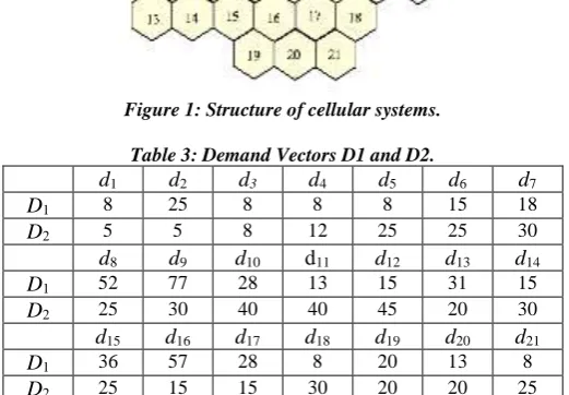
The new method described has been tested on eightbenchmark problems. The cellular structure is shown in Figure 1. Different cases have been considered with different interference constraints and demand vectors as shown in Table 3 and Table 4. The parameters shown in the tables have been explained in section 2.
Figure 1: Structure of cellular systems.
Table 3: Demand Vectors D1 and D2.
d1 d2 d3 d4 d5 d6 d7
D1 8 25 8 8 8 15 18
D2 5 5 8 12 25 25 30
d8 d9 d10 d11 d12 d13 d14
D1 52 77 28 13 15 31 15
D2 25 30 40 40 45 20 30
d15 d16 d17 d18 d19 d20 d21
D1 36 57 28 8 20 13 8
D2 25 15 15 30 20 20 25
Table 4: Different Problem cases
Problem 1 2 3 4
a.c.c 1 2 1 2
c.s.c 5 5 7 7
D1/D2 D1 D1 D1 D1
Lower bound
381 427 533 533
Problem 5 6 7 8
a.c.c 1 2 1 2
c.s.c 5 5 7 7
D1/D2 D2 D2 D2 D2
Lower Bound
221 253 309 309
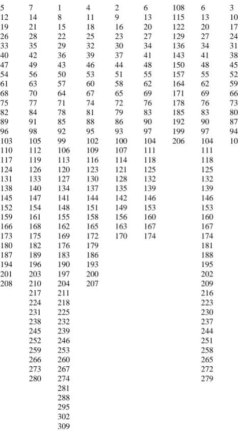
Table 5: Channel Assignment P for problem 3
5 7 1 4 2 6 108 6 3
12 14 8 11 9 13 115 13 10
19 21 15 18 16 20 122 20 17
26 28 22 25 23 27 129 27 24
33 35 29 32 30 34 136 34 31
40 42 36 39 37 41 143 41 38
47 49 43 46 44 48 150 48 45
54 56 50 53 51 55 157 55 52
61 63 57 60 58 62 164 62 59
68 70 64 67 65 69 171 69 66
75 77 71 74 72 76 178 76 73
82 84 78 81 79 83 185 83 80
89 91 85 88 86 90 192 90 87
96 98 92 95 93 97 199 97 94
103 105 99 102 100 104 206 104 101 110 112 106 109 107 111 111
117 119 113 116 114 118 118
124 126 120 123 121 125 125
131 133 127 130 128 132 132
138 140 134 137 135 139 139
145 147 141 144 142 146 146
152 154 148 151 149 153 153
159 161 155 158 156 160 160
166 168 162 165 163 167 167
173 175 169 172 170 174 174
180 182 176 179 181
187 189 183 186 188
194 196 190 193 195
201 203 197 200 202
208 210 204 207 209
217 211 216
224 218 223
231 225 230
238 232 237
245 239 244
252 246 251
259 253 258
266 260 265
273 267 272
280 274 279
281
288
295
302
Table 6: Channel Assignment Pfor problem 3
108 6 2 3 5 6 5 4 1 7 6 1 4 1 2 3 108 4 7 6 5
115 13 9 10 12 13 12 11 8 14 13 8 11 8 9 10 115 11 14 13 12 122 20 16 17 19 20 19 18 15 21 20 15 18 15 16 17 122 18 21 20 19 129 27 23 24 26 27 26 25 22 28 27 22 25 22 23 24 129 25 28 27 26 136 34 30 31 33 34 33 32 29 35 34 29 32 29 30 31 136 32 35 34 33 143 41 37 38 40 41 40 39 36 42 41 36 39 36 37 38 143 39 42 41 40 150 48 44 45 47 48 47 46 43 49 48 43 46 43 44 45 150 46 49 48 47 157 55 51 52 54 55 54 53 50 56 55 50 53 50 51 52 157 53 56 55 54 164 62 58 59 61 62 61 60 57 63 62 57 60 57 58 59 164 60 63 62 61 171 69 65 66 68 69 68 67 64 70 69 64 67 64 65 66 171 67 70 69 68 178 76 72 73 75 76 75 74 71 77 76 71 74 71 72 73 178 74 77 76 75 185 83 79 80 82 83 82 81 78 84 83 78 81 78 79 80 185 81 84 83 82 192 90 86 87 89 90 89 88 85 91 90 85 88 85 86 87 192 88 91 90 89 199 97 93 94 96 97 96 95 92 98 97 92 95 92 93 94 199 95 98 97 96 206 104 100 101 103 104 103 102 99 105 104 99 102 99 100 101 206 102 105 104 103
111 107 110 111 110 109 106 112 111 106 109 106 107 109 112 111 110
118 114 117 118 117 116 113 119 118 113 116 113 114 116 119 118 117
125 121 124 125 124 123 120 126 125 120 123 120 121 123 126 125 124
132 128 131 132 131 130 127 133 132 127 130 127 128 130 133 132 131
139 135 138 139 138 137 134 140 139 134 137 134 135 137 140 139 138
146 142 145 146 145 144 141 147 146 141 144 141 142 144 147 146 145
153 149 152 153 152 151 148 154 153 148 151 148 149 151 154 153 152
160 156 159 160 159 158 155 161 160 155 158 155 156 158 161 160 159
167 163 166 167 166 165 162 168 167 162 165 162 163 165 168 167 166
174 170 173 174 173 172 169 175 174 169 172 169 170 172 175 174 173
181 180 180 179 176 182 181 176 179 176 179 182 180
188 187 187 186 183 189 188 183 186 183 186 189 187
195 194 194 193 190 196 195 190 193 190 193 196 194
202 201 201 200 197 203 202 197 200 197 200 203 201
209 208 208 207 204 210 209 204 207 204 207 210 208
216 211 217 216 211 211 217
223 218 224 223 218 218 224
230 225 231 230 225 225 231
237 232 238 237 232 232 238
244 239 245 244 239 239 245
251 246 252 251 246 246 252
258 253 259 258 253 253 259
265 260 266 265 260 260 266
272 267 273 272 267 267 273
279 274 280 279 274 274 280
281 281 281
288 288 288
295 295 295
302 302 302
309 309 309
Table 7 : Results for Problem 8 5 3 215 1 5 3 283 215 5 283 3 1 215 215 5 3 215 5 283 5 3 12 10 222 8 12 10 290 222 12 290 10 8 222 222 12 10 222 12 290 12 10 19 17 229 15 19 17 297 229 19 297 17 15 229 229 19 17 229 19 297 19 17 26 24 236 22 26 24 304 236 26 304 24 22 236 236 26 24 236 26 304 26 24 33 31 243 29 33 31 243 33 31 29 243 243 33 31 243 33 33 31 40 38 250 36 40 38 250 40 38 36 250 250 40 38 250 40 40 38 47 45 257 43 47 45 257 47 45 43 257 257 47 45 257 47 47 45 54 52 264 50 54 52 264 54 52 50 264 264 54 52 264 54 54 52 61 59 271 57 61 59 271 61 59 57 271 271 61 59 271 61 61 59 68 66 278 64 68 66 278 68 66 64 278 278 68 66 278 68 68 66 75 73 285 71 75 73 285 75 73 71 285 285 75 73 285 75 75 73 82 80 292 78 82 80 292 82 80 78 292 292 82 80 292 82 82 80 89 87 299 85 89 87 299 89 87 85 299 299 89 87 299 89 89 87 96 94 306 92 96 94 306 96 94 92 306 306 96 94 306 96 96 94 103 101 99 103 101 103 101 99 103 101 103 103 101 110 108 106 110 108 110 108 106 110 108 110 110 108 117 115 113 117 115 117 115 113 117 115 117 117 115 124 122 120 124 122 124 122 120 124 122 124 124 122 131 129 127 131 129 131 129 127 131 129 131 131 129 138 136 134 138 136 138 136 134 138 136 138 138 136 145 143 141 145 143 145 143 141 145 143 145 145 143 152 150 148 152 150 152 150 148 152 150 152 152 150 159 157 155 159 157 159 157 155 159 157 159 159 157 166 164 162 166 164 166 164 162 166 164 166 166 164 173 171 169 173 171 173 171 169 173 171 173 173 171 180 178 176 180 178 180 178 176 180 178 180 180 178 187 185 183 187 185 187 185 183 187 185 187 187 185 194 192 190 194 192 194 192 190 194 192 194 194 192 201 199 197 201 199 201 199 197 201 199 201 201 199 208 206 204 208 206 208 206 204 208 206 208 208 206 213 211 213 213 211 213 213
220 218 220 220 218 220 220
227 225 227 227 225 227 227
234 232 234 234 232 234 234
241 239 241 241 239 241 241
248 246 248 248 246 248 248
255 253 255 255 253 255 255
262 260 262 262 260 262 262
269 267 269 269 267 269 269
276 274 276 276 274 276 276
281 281
288 288
295 295
302 302
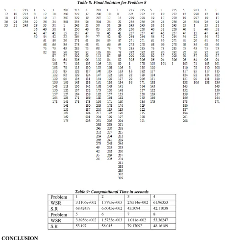
Table 8: Final Solution for Problem 8
Table 9: Computational Time in seconds
Problem 1 2 3 4
WSR 3.1106e+002 1.7795e+003 2.9514e+002 61.96353
S.R 68.42439 6.6045e+002 43.3094 42.11038
Problem 5 6 7 8
WSR 3.8956e+002 1.5733e+003 1.011e+002 53.36247
S.R 53.197 58.015 79.17092 48.16189
CONCLUSION
In this paper we have considered a new method of reducing the space by forming independent sets using the compatibility matrix. This space reduction actually helps in reducing the complexity in solving the original problem and results in a gain in time. In this method we also obtain a set of redundant frequencies assigned to particular cells. This can be used in the event that there are small changes in the demand vector.
REFERENCES
[1] R. Battiti and A. Bertossi and D. Cavallaro "A randomised saturation degree heuristic for channel assignment in cellular radio networks". IEEE Transactions on Vehicular. Technology, Vol. 50(2), pp364–374, 2001.
[2] D. Beckmann and U. Killat, "A new strategy for the application of genetic algorithms to the channel-assignment problem", IEEE Transactions on Vehicular Technology, Vol. 48(4), pp1261–1269, 1999. [3] F. Box, "A heuristic technique for assigning frequencies to mobile radio nets", IEEE Transactions on
Vehicular Technology, Vol. 27, pp. 57–64, 1978.
[5] D.J. Castelino, S. Hurley, and N.M. Stephens, "A tabu – search algorithm for frequency assignment ", Annals of Operations Research, Vol. 63, pp. 301–319, 1996.
[6] G. Chakraborty, An efficient heuristic algorithm for channel assignment problem in cellular radio network, IEEE Transactions on Vehicular Technology, Vol. 50(6), pp. 1528–1539, 2001.
[7] M. Duque-Anton, D. Kunz, and B. Ruber, "Channel-assignment for cellular radio using simulated annealing", IEEE Transactions on Vehicular Technology, Vol. 42(1), pp14–21, 1993.
[8] N. Funabiki, and Y. TAkefuji, "A neural network parallel algorithm for channel assignment in cellular radio network", IEEE Transactions on Vehicular Technology, Vol. 41(4),pp. 430–437, 1992.
[9] A. Gamst, "Some lower bounds for a class of frequency assignment problems", IEEE Transactions on Vehicular Technology,Vol. 35(1), pp. 8 – 14, 1986.
[10]A. Gamst and W. Rave, "On frequency assignment in mobile automatic telephone systems, "IEEE Proc. GLOBECOM 82, pp 309–315, 1982.
[11]S.C. Ghosh, B.P. Sinha, and N. Das, "Coalesced cap: An improved technique for frequency assignment in cellular networks, " IEEE Transactions on Vehicular Technology, Vol. 55(2),pp. 640–653, 2006. [12]F. Glover and M. Laguna, "Tabu search", chapter 3. In: Reeves, C.R.(ed) Modern heuristic techniques
for combinatorial problems, McGraw-Hill, pp.70–150, 1995.
[13]W.K. Hale, Frequency assignment: Theory and applications, Proc. IEEE, Vol. 68(0), pp.1497–1514, 1980.
[14]T.M Ko, A frequency selective insertion strategy for fixed channel assignment, Proc. 5th IEEE Int. Symp. Personnal Indoor and Mobile Radio Communications, The Hague, The Netherlands, pp. 311–314, 1994. [15]D. Kunz, Channel-assignment for cellular radio using neuralnetworks, IEEE Transactions on Vehicular
Technology, Vol. 40, pp. 188– 193, 1991.
[16]M. Laguna, R. Marti, and V. Campos, Intensification and diversification with elite tabu search solutions for the linear ordering problem, Computers and Operations Research, Vol. 26, pp. 1217–1230, 1999. [17]R. Montemanni, and J.N.J. Moon, and D.H. Smith, An improved tabu search algorithm for the fixed
spectrum assignment problem. IEEE Transactions on Vehicular Techology, Vol. 52(3), pp. 891–901, 2003.
[18]C.Y. Ngo, and V.O.K. Li, Fixed channel assignment in cellular radio networks using a modified genetic algorithm, IEEE Transactions on Vehicular Technology, Vol. 26:1 , pp. 163–172, 1998.
[19]L.M.S.J. Revuelta, A new adaptive genetic algorithm for fixed channel assignment, Information Sciences, Vol. 177, pp.2655–2678, 2007.
[20]Y. Saad, A multi-elimination ILU pre-conditioner for general sparse matrices, SIAM J Sci. Comput., Vol. 17(4), pp. 830–837, 1996.
[21]K.N. Sivaranjan, R.J. McEliece, and J.W. Ketchum, Channel assignment in cellular radio. IEEE Veh. Tech. Conf, VTC 89, pp.846–850, 1989.
[22]K. Smith, and M.Palaniswami, Static and dynamic channel assignment using neural network. IEEE J. Sel. Commun., Vol.40(2),pp. 238–249, 1997.
[23]D. W. Tcha, J. H. Kwon, T. J. Choi, and S. H. Oh, Perturbation minimising frequency assignment in a changing TDMA/FDMA cellular environment. IEEE Transantions on Vehicular Technology, Vol. 49(2), pp.390–396, 2000.
[24]W. Wang and C.K. Rushforth, An adaptive local search algorithm for the channel assignment problem (cap). IEEE Transactions on Vehicular Technology, Vol. 45, pp. 459–466, 1996.