SPOTS Calibration Example
C. Sebastian1, 2a and E. A. Patterson1, 2, 3
1Composite Vehicle Research Center, Michigan State University, East Lansing, MI USA 2Department of Mechanical Engineering, Michigan State University
3Department of Chemical Engineering and Materials Science, Michigan State University
Abstract. The results are presented using the procedure outlined by the Standardisation Project for Optical Techniques of Strain measurement to calibrate a digital image correlation system. The process involves comparing the experimental data obtained with the optical measurement system to the theoretical values for a specially designed specimen. The standard states the criteria which must be met in order to achieve successful calibration, in addition to quantifying the measurement uncertainty in the system. The system was evaluated at three different displacement load levels, generating strain ranges from 289 strain to 2110 strain. At the 289 strain range, the calibration uncertainty was found to be 14.1 strain, and at the 2110 strain range it was found to be 28.9 strain. This calibration procedure was performed without painting a speckle pattern on the surface of the metal. Instead, the specimen surface was prepared using different grades of grit paper to produce the desired texture.
1 Introduction
In 2007, the Standardisation Project for Optical Techniques of Strain measurement (SPOTS) published a method for the calibration of optical strain measurement systems using a specially designed monolithic specimen which consisted of a beam in four-point bending. This draft standard [1], ‘Calibration and Assessment of Optical Strain Measurement Systems, Part I,’ along with an example performed on an ESPI system [2], were used as the guidelines to perform this calibration.
The system that was calibrated is a Q-400 digital image correlation system (Dantec Dynamics, Ulm, Germany). The basic procedure involved first using strain gages bonded to the top and bottom surfaces of the beam to determine correction factors which account for the inherent constraints imposed by the monolithic design of the specimen. The specimen was then loaded via displacement control, and strain fields were obtained using the DIC system at three increments of applied displacement, and the measured strains were compared to the predicted values.
2 Methods
The calibration specimen, or reference material, was designed by the SPOTS consortium [1] to be easily scalable and to yield consistent results. To achieve these goals, the specimen is made from a
a
e-mail : [email protected]
single piece of material which does not allow the beam to be supported by rollers or knife edges. Hence, the strain field in the gage section of the beam is modified slightly by both a lateral constraint (which shifts the neutral axis in the positive strain direction) and a bending moment (which causes a proportional change across the entire field). The bending strain in the gage section, as a function of the distance from the neutral axis perpendicular to the applied load can be described as,
)
(
6
2K
H
ky
W
v
xx (1)
where k corrects for the imposed moment, and corrects for the translational constraint and y is the distance from the neutral axis.
In order to determine the correction factors k and , strain gages were bonded to the top and bottom surfaces of the calibration specimen in the gage section. The thickness of the calibration specimen used was only 5mm, so due to clearance and space issues, single axis gages were applied to measure the strain. Each gage was then connected to a strain indicator (Measurements Group P-3500, Raleigh, NC). To measure the relative applied displacement in the specimen, aluminum blocks were machined to hold a digital indicator (Mitutoyo 543-392, Kawasaki-shi, Japan) on each side of the specimen. The total displacement of the specimen was taken as an average of the two indicators. The digital indicators were purchased with NIST traceable calibration certificates.
The specimen was mounted into the load frame (MTS 810, Eden Prairie, MN) using the pre-drilled holes, such that it could be loaded in tension. The top grip of the load frame is fixed while the bottom grip displaces, so the specimen was mounted “upside down” in order to minimize rigid body movements of the specimen. To remove any slack in the system, a 1-2 m pre-load was applied to the specimen before starting the test. The load frame was programmed to load the specimen at 0.3 mm/min for a total displacement of 0.3 mm. Data was acquired at 2 second intervals.
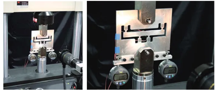
Fig. 1. The calibration specimen installed in the MTS load frame (left). Close-up of the calibration specimen showing the ring light and the strain gages (right).
14th International Conference on Experimental Mechanics
3 Results
Figure 2 shows the results of the first part of the calibration procedure in which the correction factors k and K were determined. The quantities Ymax and Ymin are the maximum and minimum strain values at the outer faces of the beam obtained with the strain gages. Ymax+Ymin and Ymax-Ymin are plotted as a function of applied displacement load from 0 to 180 m.
-2500 -2000 -1500 -1000 -500 0 500
0 20 40 60 80 100 120 140 160 180 200
Displacement (m)
xx
(
st
ra
in
)
Ymax+Ymin
Ymax-Ymin
Fig. 2. Plot of Ymax+Ymin and Ymax-Yminas a function of applied displacement used to calculate the correction factors k and . The strain data was obtained from strain gages bonded to the top and bottom surfaces of the beam in the gage section.
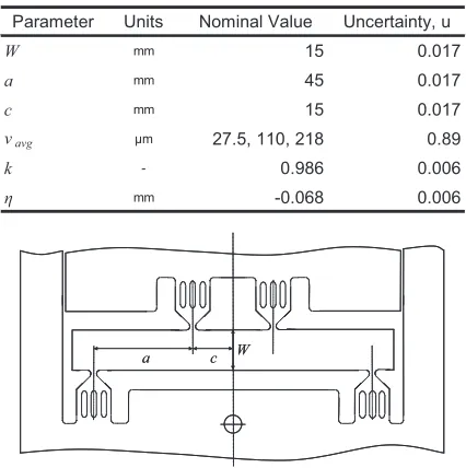
Table 1 summarizes the values and uncertainty factors for the critical dimensions of the beam and the correction factors. A drawing of the calibration specimen is shown in Figure 3, and illustrates the dimensions W, a, and c. The uncertainty of these dimensions is estimated from the manufacturing tolerances. The values for the applied displacement were provided from the calibration certificates of the digital indicators. The uncertainty for k and were calculated according to the SPOTS standard assuming a rectangular distribution in the last digit.
Table 1. The critical dimensions of the calibration specimen and their associated uncertainties.
Parameter Units Nominal Value Uncertainty, u
W mm 15 0.017
a mm 45 0.017
c mm 15 0.017
vavg m 27.5, 110, 218 0.89
k - 0.986 0.006
mm -0.068 0.006
W c
a c W
a
In Figure 4, the strain measured by the digital image correlation system is plotted against the calculated values using equation (1) for the largest displacement load step (218 m). The strain map that was obtained from the digital image correlation system is also shown.
-1500 -1000 -500 0 500 1000 1500
-8 -6 -4 -2 0 2 4 6 8
y (mm) Strain (strain)
DIC
Strain gage
Difference
Fig. 4. Measured and calculated strain values for the 218 m displacement load (left). The strain map associated with the 218 m displacement generated by the DIC system (right).
For each of the load steps, fit parameters and were calculated by using the linear least-squares fit method described in the SPOTS standard. The uncertainty of and were also calculated, and the range formed by ±2u forms a 95% confidence interval for each of the parameters. Table 2 summarizes this data.
Table 2. Summary of the fit parameters calculated for each of the displacements, as well as their associated 95% confidence levels.
Fit Parameter Units 27.5 110 218
strain -3.2 2.0 11.9
u() strain 1.29 1.69 2.66
95% Confidence Interval () strain ±2.57 ±3.38 ±5.36
strain mm-1 -4.4 -4.9 -3.6
u() strain mm-1 0.32 0.42 0.67
95% Confidence Interval () strain mm-1
±0.65 ±0.85 ±1.34
Applied displacement, vavg (m)
14th International Conference on Experimental Mechanics -200 -150 -100 -50 0 50 100 150 200
-8 -6 -4 -2 0 2 4 6 8
y (mm) Difference ()
±2uCS
k+ky
(k+ky) ± 2u(dk)
±2uCS
k+ky
(k+ky)±2u(dk)
-200 -150 -100 -50 0 50 100 150 200
-8 -6 -4 -2 0 2 4 6 8
y (mm) Difference ()
±2uCS
k+ky
(k+ky) ± 2u(dk)
±2uCS
k+ky
(k+ky)±2u(dk)
-200 -150 -100 -50 0 50 100 150 200
-8 -6 -4 -2 0 2 4 6 8
y (mm) Diff erence ()
±2uCS
k+ky
(k+ky) ± 2u(dk)
±2uCS
k+ky
(k+ky)±2u(dk)
-200 -150 -100 -50 0 50 100 150 200
-8 -6 -4 -2 0 2 4 6 8
y (mm) Diff erence ()
±2uCS
k+ky
(k+ky) ± 2u(dk)
±2uCS
k+ky
(k+ky)±2u(dk)
-200 -150 -100 -50 0 50 100 150 200
-8 -6 -4 -2 0 2 4 6 8
y (mm) Difference ()
±2uCS
k+ky
(k+ky) ± 2u(dk)
±2uCS
k+ky
(k+ky)±2u(dk)
-200 -150 -100 -50 0 50 100 150 200
-8 -6 -4 -2 0 2 4 6 8
y (mm) Difference ()
±2uCS
k+ky
(k+ky) ± 2u(dk)
±2uCS
k+ky
(k+ky)±2u(dk)
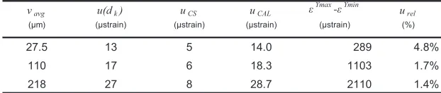
The system’s overall calibration uncertainty, uCAL, was calculated using the uncertainty from the calibration specimen uCS and from the strain measurements u(dk). These values were all calculated using the maximum strain value from each of the load steps. In addition, the relative uncertainty urel was found using the procedure described in [2]. Table 3 shows that the primary source of uncertainty contributing to uCAL is from the strain measurement and not the calibration specimen.
Table 3. Summary of the uncertainty values for each of the load steps. The uncertainty values listed are for the maximum strain of each load step.
vavg u(dk) uCS uCAL
Ymax
-Ymin urel
(m) (strain) (strain) (strain) (strain) (%)
27.5 13 5 14.0 289 4.8%
110 17 6 18.3 1103 1.7%
218 27 8 28.7 2110 1.4%
4 Discussion
The SPOTS procedure gives values for the correction factors from FEA results, but it also allows them to be found experimentally, as was done in this study. For a specimen with a beam depth of 15mm, the FEA results show that k=0.94 and =-0.10. The values obtained experimentally were very close to these, with k=0.986 and =-0.068. Initially when determining the correction factors, the strain gages were zeroed with the specimen laying flat on the table. The specimen was then mounted in the load frame and the indicators were installed and zeroed. It was later found that the indicators were causing a few m of displacement on the specimen due to their weight. In order to eliminate this, the indicators were mounted and zeroed at the same time as the strain gages, when the specimen was laying flat on a table.
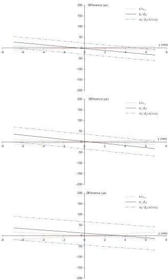
For all three of the displacement load steps, there is complete overlap between the expanded uncertainty of the reference material and the mean residual deviations k + ky. According to the SPOTS standard, this qualifies as acceptable, requiring no adjustment to the instrument. However, the standard also states that k and k should be less than twice their respective uncertainty. When |k|>2u(k), this indicates a statistically significant offset in the calibration. When |k|>2u(k), it implies there is a statistically significant deviation in the calibration. The data listed in Table 2 shows that both of these cases were true for this calibration. It is also interesting to note that the value for increases as a function of applied displacement, where as the value for remains relatively constant.
5 Conclusions
A digital image correlation system has been calibrated following the procedure set forth in the SPOTS standard and found to provide acceptable results. The calibration uncertainty data calculated from the procedure will be important in qualifying future test measurement made with the system. It was also determined that good results can be achieved without having to use a speckle pattern on the surface of the object of interest.
References
1. SPOTS Consortium (2007) Standardised Project for Optical Techniques of Strain
Measurement see http://www.opticalstrain.org
2. M. P. Whelan, D. Albrecht, E. Hack and E. A. Patterson, Calibration of a Speckle Interferometry Full-Field Strain Measurement System (Strain 44:180-190, 2008)
3. E. A. Patterson, E. Hack, P. Brailly, R. Burguette, Q. Saleem, T. Siebert, R. A. Tomlinson and M. P. Whelan, Calibration and evaluation of optical systems for full-field strain measurement (Optics and Lasers in Engineering 45:550-564, 2007)