RHEOLOGY AND FLOW OF MUCUS IN HUMAN BRONCHIAL EPITHELIAL CELL CULTURES
Yuan Jin
A dissertation submitted to the faculty at the University of North Carolina at Chapel Hill in partial fulfillment of the requirements for the degree of Doctor of Philosophy in the Department of
Mathematics.
Chapel Hill 2015
Approved by:
M. Gregory Forest
Paula Vasquez
David Hill
Jingfang Huang
c 2015 Yuan Jin
ABSTRACT
Yuan Jin: Rheology and Flow of Mucus in Human Bronchial Epithelial Cell Cultures
(Under the direction of M. Gregory Forest)
The propulsion of mucus in human airways toward the trachea by the collective and coordinated
action of cilia, known as mucociliary clearance, remains an outstanding modeling and computational
challenge. A model system for mucociliary clearance is provided by human bronchial epithelial (HBE)
cell cultures that generate macroscopic mean rotational flow. We coarse grain the coordinated
cilia propulsion into an imposed dynamic velocity condition on the flat base of a cylinder. A
multi-mode Giseskus nonlinear viscoelastic constitutive model derived from rheological data of
mucus is employed for the mucus layer. The full system of governing equations for the transient and
stationary axisymmetric flow field and air-mucus interface is solved numerically. Our modeling is
the first step toward a platform for several purposes: to test accuracy of the constitutive modeling
of mucus; to build a faithful model of the cilia-mucus boundary condition; to simulate both the
flow and stress fields throughout the mucus layer; to explore the linear and nonlinear viscoelastic
behavior of the mucus flow; and to explore the advection-diffusion process of a drug concentration
dropped at the surface of the cell culture, and illustrate how the absorption by the bottom plate
ACKNOWLEDGMENTS
I would like to express my deep appreciation and gratitude to my advisor Dr. Forest, for his
extraordinary guidance, support and encouragement during my graduate study. I’d also like to
thank my entire committee: Paula Vasquez, David Hill, Jingfang Huang and Laura Miller.
I am so thankful for the love and encouragement that my wife Lu had been giving me during
the last five years. I am also very grateful for the support of my parents, who have always believed
TABLE OF CONTENTS
LIST OF FIGURES . . . vi
Chapter 1. RHEOLOGY OF MUCUS . . . 1
1.1 Introduction to Viscoelastic Fluid . . . 1
1.2 Small Amplitude Oscillatory Shear . . . 1
1.3 Simple Mechanical Models for Viscoelastic Materials . . . 2
1.3.1 Nonlinear Constitutive Models . . . 4
1.4 Large Amplitude Oscillatory Shear Analysis . . . 5
Chapter 2. MODELING OF MUCUS FLOW IN HBE CELL CULTURE . . . . 7
2.1 Introduction . . . 7
2.1.1 HBE Cell Cultures . . . 8
2.1.2 Mucus Flow in HBE Cell Cultures . . . 10
2.1.3 Axisymmetric Assumption . . . 11
2.2 Model Equations . . . 13
2.2.1 Nondimensionalizaion . . . 14
2.3 Data-derived Nonlinear Constitutive Model . . . 14
2.4 Coarse-graining of the Cilia Carpet Driving Conditions . . . 15
2.5 Numerical Methods . . . 18
2.6 Results . . . 20
2.6.1 Swirling Flow: Compare Newtonian Fluid with Viscoelastic Fluid . . . 20
2.6.2 Numerical Mucus Flow in Cell Culture . . . 21
2.7 Large Amplitude Oscillatory Shear(LAOS) Analysis of Nonlinearity . . . 30
2.8 Advection-diffusion of Drug Concentrations . . . 34
2.9.1 Convergence . . . 44
2.9.2 Benchmarking . . . 44
Chapter 3. CONCLUSIONS . . . 51
LIST OF FIGURES
1.1 ”Spring” element of solid-like behavior . . . 2
1.2 ”Dashpot” element of liquid-like behavior . . . 3
1.3 Illustration of Maxwell model . . . 3
1.4 Illustration of Kelvin-Voigt model . . . 4
1.5 Illustration of Jeffrey model . . . 4
2.1 Mucociliary clearance in human airway (David Hill) . . . 8
2.2 Schematic of an HBE Cell Culture . . . 9
2.3 HBE Cell Culture Geometry (John Melnick) . . . 10
2.4 Demonstration of rotational mucus transport in HBE cell cultures. (A) Traces of 1 mm fluorescent micro-spheres at the culture surface from a 5 second time lapse exposure. (B) Linear velocities of the particles versus distance from the center of rotation. Data extrapolated from [21]. With the rotational flow, the mucus tend to swell up in the middle of the HBE cell culture, forming a dome shape for the free surface of the mucus flow, see Figure 2.5. . . 11
2.5 Surface shape of an HBE cell culture shows the dome at the center [21] . . . 11
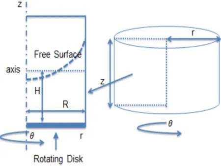
2.6 HBE cell culture in cylindrical coordinates and reduction from 3D cylinder to 2D rectangular region based on the axisymmetric assumption . . . 12
2.7 (A) Linear dynamic storage (G) and loss (G) moduli data (solid, open dots) for 2.5wt% HBE mucus across a frequency range, together with the corresponding fit to 5 UCM modes. (B) Viscosity vs. shear rate data for 2.5wt% HBE mucus and corresponding fit to a sum of 5 Giesekus modes. The curve shown is the best fit under the condition 0α0.5. Model parameters are given in Table 1. Data courtesy of Jeremy Cribb and David Hill. . . 15
2.8 Movement of a single cilium: power stroke and recovery stroke. Data replotted from [23] and adapted from [10]. . . 16
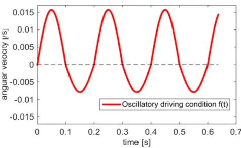
2.9 The oscillatory driving condition f(t) imposed at the bottom plate to mimic cilia power and return strokes and match experimental observation . . . 17
2.11 Transient process of the flow field for a Newtonian fluid; the velocity field in the plot is the secondary flow (ur vs uz) and the color map in the background is the primary
flowuθ . . . 22
2.12 Transient process of the flow field for a a single mode UCM fluid; the velocity field in the plot is the secondary flow (ur vs uz) and the color map in the background is the
primary flow uθ . . . 23
2.13 Transient process of the flow field for a single mode Giesekus fluid withα= 0.3; the velocity field in the plot is the secondary flow (ur vs uz) and the color map in the
background is the primary flow uθ . . . 24
2.14 Transient process of the flow field for a 5 modes Giesekus fluid with parameters specified in Table 2.3; the velocity field in the plot is the secondary flow (ur vs uz)
and the color map in the background is the primary flowuθ . . . 25
2.15 The stationary secondary flow field and streamlines for nonlinear viscoelastic mucus model in the middle of the cell culture (left) and at the edge of the cell culture (right). 26
2.16 Free surface shape at steady state for the swirling flow with different types of fluids 26
2.17 Mass transport flux rate across theθ= 0 plane for the swirling flow with different types of fluids . . . 27
2.18 Flow field for a 5 modes Giesekus fluid with parameters specified in Table 2.3 with the oscillatory driving condition in Section 2.4; the velocity field in the plot is the secondary flow (ur vs uz) . . . 28
2.19 Mass transport flux rate across oneθ= 0 plane with oscillatory driving condition for 5 modes Giesekus fluid with parameters specified in Table 2.3; . . . 29
2.20 Left: Velocity envelopes in angular direction at the edge of cell culture; Right: displacement in angular direction at the edge of cell culture at different heights for 5 modes Giesekus fluid with parameters specified in Table 2.3; . . . 29
2.21 Left: Driving condition foruθwhereuθis a sinusoidal function of time; Right: Driving
condition for uθ where shear strain is a sinusoidal function of time . . . 31
2.22 The envelopes of shear strain(left) and shear stress(right) across the gap atr= 0.5∗R 32
2.23 Normalized Lissajous curves of shear stress VS shear strain (left) and shear stress VS shear rate (right) at different positions of the cell culture . . . 32
2.24 Storage ModulusG0 (Left) and Loss ModulusG00 (Right) everywhere in the cell culture 33
2.26 LAOS analysis for nonlinear viscoelasticity at r = 0.4∗R and h = 0.4∗H with
R= 5mm. . . 35
2.27 Characterizing the linear and nonlinear regime for mucus flow with respect to the aspect-ratio and mean drivinguθ atr = 0.5∗R . . . 36
2.28 Initial drug concentration type 1; Blue disk shows the surface of the cell culture; red disk is the initial concentration of unit drug at the surface. . . 37
2.29 The advection-diffusion of the drug concentration withP e= 0.1 in the mucus flow . 39 2.30 The advection-diffusion of the drug concentration withP e= 10 in the mucus flow . 40 2.31 The percentages of the drug concentration absorbed by outer part” of the bottom plate in the end versus Peclet number P e . . . 41
2.32 The time it takes for 95% of the drug concentration to be absorbed by the bottom of the cell culture versus Peclet number P e . . . 41
2.33 Initial drug concentration type 1; Blue disk shows the surface of the cell culture; red line is the initial concentration of unit drug at the surface. . . 42
2.34 Initial drug concentration type 1; Blue disk shows the bottom of the cell culture; the red fan stands for the area where−12π < θ < 12π. . . 43
2.35 Percentage of drug concentration absorbed by the fan area in the bottom plate versus Peclet number P e. . . 43
2.36 Convergence test: ur at the middle height for a single UCM fluid . . . 45
2.37 Convergence test: uz at the middle height for a single UCM fluid . . . 45
2.38 Convergence test: uthetaat the middle height for a single UCM fluid . . . 46
2.39 Convergence test: free surface shape for a single UCM fluid . . . 46
2.40 The evolution of the tangential velocities after the stop of the rotating disk for a single mode UCM fluid . . . 47
2.41 Tangential velocity distribution for a single mode UCM fluid after stabilization . . . 47
2.42 Illustration of Quelleffekt . . . 48
2.44 Displacement h of the upper surface along the axis of symmetry as a function of H for a single mode Giesekus fluid with α= 0.3. . . 49
CHAPTER 1
RHEOLOGY OF MUCUS
1.1 Introduction to Viscoelastic Fluid
For elastic solids, when undergoing deformation, the stress is always proportional to strain
(defor-mation) but independent of the rate of the strain, in accordance with the Hooke’s law. For viscous
fluids, the stress is proportional to the rate of the strain, but independent of the strain itself, in
accordance with the Newton’s Law. Viscoelastic materials are intermediate between elastic solids
and viscous fluids and may exhibit behaviors which combine liquid-like and solid-like characteristics
[7] [15] [18]. Examples of viscoelastic materials may include food, polymers, bio-fluids, as well as
the mucus inside human air-way and lung that we will focus on in Chapter 2. One example of
viscoelastic behavior is the so-called Weissenberg or rod-climbing effect [5]. When a rod is set to
rotate in a Newtonian fluid, the inertial force push the material to the outside of the container.
However, for some viscoelastic fluids, stress will develop along the normal axes of the flow field
and push the fluids to ”climb” up along the rotating rod. The relations between stress, strain
and their time dependences of a viscoelastic material are described by the constitutive equations
[7] [15] [18]. In this chapter, we illustrate the dynamic modulus for viscoelastic fluid in small
amplitude oscillatory shear (SAOS) (Section 1.2). And we review the techniques for modeling
nonlinear viscoelastic properties in large amplitude oscillatory shear (LAOS) (Section 1.2). Both
the SAOS and LAOS are rheological experiments that are commonly used to probe the viscoelastic
properties of complex fluids. We introduce three simple linear constitutive models (Section 1.3) and
two nonlinear viscoelastic models (Section 1.3).
1.2 Small Amplitude Oscillatory Shear
When viscoelastic materials are subjected to a small amplitude sinusoidally oscillating strain, the
phase (as it would for a viscous liquid), but is somewhere in between [15].
In small amplitude oscillatory shear (SAOS) experiment [15], one imposes a sinusoidal strain
and measure the resulted stress. The strain isγ =γ0sin(ωt), the strain rate is ˙γ =γ0cos(ωt), and
the resulted stress can be decomposed as,
σ = G∗γ0sin(ωt+δ)
= G∗γ0[sin(ωt) cos(δ) + cos(ωt)sin(δ)]
= (G∗cos(δ))·γ0sin(ωt) + (G∗sin(δ))·γ0cos(ωt)
= [G0 ·sin(ωt) +G00·cos(ωt)]γ0
= G0γ+ G
00
w γ˙
G0 and G” are the storage and loss modulus of the viscoelastic materials. The storage modulus
measure the stored energy, representing the elastic portion; and the loss modulus measure energy
dissipated as heat, representing the viscous portion.
1.3 Simple Mechanical Models for Viscoelastic Materials
Solid-like behavior is described by Hooke’s Law, and represented by a spring [Figure 1.1] mechanical
analog.
τ =Gγ
where τ is the stress,G is the elastic modulus of the material, andγ is the strain.
Figure 1.1: ”Spring” element of solid-like behavior
Liquid-like behavior is described by Newton’s law, and represented by using a dashpot [Figure 1.2]
mechanical analog:
where τ is the stress,η is the viscosity of the material, and ˙γ is the strain rate.
Figure 1.2: ”Dashpot” element of liquid-like behavior
Viscoelastic behavior has elastic and viscous components, and can be modeled as linear
com-binations of springs and dashpots, respectively. Each model differs in the arrangement of these
elements.
• Maxwell model
Constitutive equation,
ηγ˙ = η Gσ˙ +σ
Figure 1.3: Illustration of Maxwell model
• Kelvin-Voigt model
Constitutive equation,
ηγ˙+Gγ =σ
• Jeffrey model
Constitutive equation,
Figure 1.4: Illustration of Kelvin-Voigt model
Figure 1.5: Illustration of Jeffrey model
1.3.1 Nonlinear Constitutive Models
• Giesekus model
The Giesekus model [8] is based on the concept of anisotropic drag between the solvent and
polymer molecules. The latter is represented by Hookean dumbbells immersed in a Newtonian
solvent. The constitutive equation is
λτ(1)+τ+ αgλ
ηp
τ·τ = 2ηpD,
where αg is a so-called mobility parameter; λis the fluid relaxation time; and ηp =η0−ηs
is the polymer viscosity, with η0 the zero shear viscosity. The strain rate tensor is 2D =
(∇v)T + (∇v), and the upper convected derivative is defined as,
(·)(1)= ∂
∂t−v·∇(·)−(∇v)
T ·(·)−(·)·(∇v).
• Rolie-Poly model
The Rolie-Poly model [17] also arises from molecular theory, where the polymer molecules are
convection, and convective constraint release mechanisms. In differential form the model is
given by
λτ(1)+τ+ 2 λ λR
(1−ftr) [(1 +βRPftr)τ+G0I] = 2ηpD,
where
ftr = s
3 3 +tr(τ/G0).
Here the plateau modulus is G0 =η0/λand the two relaxation times in the model are the
reptation timeλand the retraction time λR.
1.4 Large Amplitude Oscillatory Shear Analysis
For oscillatory shear experiment, when the strain amplitude is sufficiently large, the material response
will become nonlinear and the SAOS modulus G0 andG” are no longer sufficient. BecauseG0 andG”
in SAOS are based on the assumption that the stress response is purely sinusoidal (linear). However,
a nonlinear stress response is not a perfect sinusoid and the viscoelastic modulus are not uniquely
defined. Therefore, other techniques are needed for quantifying the nonlinear material response
under LAOS deformation [5].
The mathematical structure of the nonlinear stress response is fully captured by the higher
Fourier harmonics,
σ=γ0
X
n:odd
G0nsin(nωt) +G00ncos(nωt)
The intensity of the higher harmonics could work as a measure of nonlinearity, but these coefficients
lack a clear physical interpretation [5].
Another qualitative measure of nonlinear viscoelastic response is the Lissajous curves [22] [5].
Elastic Lissajous curves show the plot of oscillatory stress versus input strain, whereas in viscous
Lissajous curves one plots the stress against the rate of strain. For an elastic solid, the elastic
Lissajous curves are represented by straight lines and viscous Lissajous curves by circles, while the
opposite is true for a viscous fluid. In the small amplitude regime for a generic viscoelastic fluid,
both Lissajous curves are ellipses. Departures from an ellipse signal that the nonlinear LAOS regime
has been reached.
on geometric considerations. They showed that these contributions are one-to-one functions of the
strain and the strain rate respectively, so that they become one-dimensional lines in the elastic and
viscous Lissajous curves. This overcomes the problem of characterizing two-dimensional ellipses in
the Lissajous curves. They proved that for LAOS there exists one unique decomposition(denote
x=γ and y= ˙γ/ω)
σ(x, y) =σ0(x, γ0) +σ00(y, γ0)
where σ0(x) and σ00(y) represent ”elastic” stress and ”viscous”.
Ewoldt et al. [6] then used Chebyshev polynomials as orthonormal basis functions to further
decompose these stresses into harmonic components having physical interpretations.
σ0(x) =γ0
X
n odd
en(ω, γ0)Tn(x)
σ00(y) =γ0
X
n odd
vn(ω, γ0)Tn(y)
They developed several nonlinear metrics for LAOS using the Chebyshev coefficient above. These
metrics also have a direct geometrical representation in the Lissajous curves, and have the advantage
of not being based on individual harmonic contributions.For example, e3 > 0 indicates
strain-stiffening, e3 <0 indicates strain-softening, v3 >0 indicates shear-thickening, and v3 <0 indicates
CHAPTER 2
MODELING OF MUCUS FLOW IN HBE CELL CULTURE
2.1 Introduction
The propulsion of mucus in human airways to the trachea by the collective, coordinated action
of cilia, known as mucociliary clearance, remains an outstanding modeling and computational
challenge. A predictive model has medical relevance since failure to clear mucus from the airways
leads to chronic, even fatal, lung infections. Additionally, the causal relationship between mucus
rheology and mucociliary clearance remains an open problem in the field. The three major modeling
components of mucociliary clearance are: a constitutive model for mucus based on rheological data,
a mechanism (forcing condition) for mucus propulsion either by individual cilia or carpets of cilia,
and numerical methods to solve the full system of equations [25]. Validation of each component
in airway simulations is essentially impossible due to the lack of in vivo experimental data and
resolution of airway mucus transport.
A transformative model system for the study of mucociliary clearance is provided by human
bronchial epithelial (HBE) cell cultures, whereby an epithelial tissue, a layer of fluid surrounding
the cilia, and an overlying mucus layer, are grown in a cylindrical dish [Figure 2.2] [9]. These cell
cultures generate macroscopic mean flow in a clockwise or counterclockwise motion, forming what
appears from above as a rotating vortex or mucus hurricane [Figure 2.4].
Our goal here is to simulate the flow of mucus in a HBE cell culture, both as a first modeling
step to aid experimental studies, and as a constitutive model test for mucus against cell culture
observations. We employ a multi-mode Giesekus nonlinear viscoelastic constitutive law for the mucus
layer. The Giesekus model is a canonical nonlinear constitutive model that captures shear thinning
and first and second normal stress generation in shear [8]. In this chapter, multiple modes are
used to approximate the broad relaxation spectrum of mucus. We coarse grain the cilia propulsion
the air-mucus interface is treated as a free boundary, whose shape is investigated with the effect
of surface tension. We develop a numerical algorithm and implement it to solve the full system of
governing equations for the transient and stationary axisymmetric flow field and air-mucus interface,
and explore the mass transport of mucus as a function of the Giesekus constitutive properties and the
imposed driving condition at the lower plate. We studied the nonlinear viscoelastic properties of our
multi-mode Giesekus constitutive model in the cell culture. And we explore the advection-diffusion
process of a drug concentration dropped at the surface of the cell culture.
Figure 2.1: Mucociliary clearance in human airway (David Hill)
2.1.1 HBE Cell Cultures
The primary human bronchial epithelial (HBE) airway cell culture is an invaluable model system of
the human airway. These cultures, developed by Lencher and coworkers [16], grow to confluence
with cell differentiation into goblet cells that produce mucin proteins and ciliated cells that sprout
active cilia, forming epithelial tissue that draws nutrients and water from the reservoir below the
membrane. Within weeks, an air-mucus interface forms over a mucus layer of∼10−50 microns, with
a periciliary liquid layer (PCL) between mucus and tissue approximately 7 microns thick. Ciliated
cells (∼200 per ciliated cell, each∼8 microns long at full extension of the power stroke) coordinate
their individual power-return stroke with∼ 10−15Hz frequency, propelling the mucus layer in the
and thus the expression mucus hurricanes was born [Figure 2.4A]. Once coordinated transport of the
mucus layer is established, fluorescent tracer particles [19], [2], gold nanorods [21], or endogenous
cellular debris [21], [3] can be tracked to gain flow profile information. For cultures whose cilia
synchronize and transport mucus around the dish, a true ex vivo model assay is provided for a
detailed study of a wide range of pulmonary physiology. Cells are obtained from donors of various
disease populations including Chronic Obstructive Pulmonary Disease (COPD) and Cystic Fibrosis,
reproducing acquired and genetic mutations, thereby serving as a model for disease pathology and
as a testbed for flow and rheological consequences of drug or physical therapies.
Figure 2.2 shows a picture of one HBE cell culture from David Hill’s lab. Figure 2.3 illustrates
the detailed dimensions of the HBE cell culture. The radius of the cell culture is around 13.3mm.
The height of cell culture is around 12.3mm, and the depth of the mucus layer in HBE cell cultures
ranges from 10−50µm[11]. Therefore, we have a relatively large aspect-ratio of the cell culture
radius over the depth of the mucus layer, which ranges from 1000−50.
Figure 2.2: Schematic of an HBE Cell Culture
In this work, experimental data from micro and macrorheology are used to construct a nonlinear
constitutive model of mucus. We refer to recent studies of biochemical composition [14] [9] [11]
Figure 2.3: HBE Cell Culture Geometry (John Melnick)
of cilia-mucus propulsion, and idealize the forcing mechanism of the power and return stroke as
though the cilia were uniformly synchronized. The actual momentum transfer mechanism between
the PCL and mucus layers remains one of the most important unsolved problems in lung mechanics.
We do not address this problem in the current paper, since to do so would require detailed modeling
of fully three-dimensional fluid flow, single and coordinated nonlinear viscoelastic fluid-structure
interactions, and a heterogeneous, dynamic, cilia-PCL-mucus boundary condition. Instead, we
coarse grain the PCL as a moving solid boundary, averaging out the scales of the coordinated cilia
to study the mean mucus transport features due to a homogeneous dynamic cilia carpet consisting
of a power stroke and a return stroke.
2.1.2 Mucus Flow in HBE Cell Cultures
Due to the cylindrical geometry of the culture wares used in the growth of HBE cultures, mucus
transport in these system is rotational, forming so-called mucus ”hurricanes” [Figure 2.4A] [19] that
serve as the basis of the modeling of mucociliary transport presented herein. Experiments reveal a
center as shown in Figure 2.4B.
Figure 2.4: Demonstration of rotational mucus transport in HBE cell cultures. (A) Traces of 1 mm fluorescent micro-spheres at the culture surface from a 5 second time lapse exposure. (B) Linear velocities of the particles versus distance from the center of rotation. Data extrapolated from [21]. With the rotational flow, the mucus tend to swell up in the middle of the HBE cell culture, forming a dome shape for the free surface of the mucus flow, see Figure 2.5.
Also note here that though the cilia carpet and mucus layer cover the whole cell culture, the
observed mucus ”hurricane” only forms at the middle part of the cell culture, which makes the
radius of the mucus ”hurricane” less than 13.3mmand could be as low as around 4mm.
Figure 2.5: Surface shape of an HBE cell culture shows the dome at the center [21]
2.1.3 Axisymmetric Assumption
As noted above, for this study we suppress heterogeneity of the cilia forcing condition, tantamount
to a two-dimensional long-wave limit of the ciliary metachronal wave. The ciliated carpet is thereby
mimics the power and return strokes of cilia. This coarse-graining of the cilia carpet is self-consistent
with axisymmetry of the three flow variables, pressure, and free surface, affording a reduction in the
computation from three to two space dimensions, as shown in Figure 2.6.
With the axisymmetric assumption, the computational domain consists of a cylinder of radius
R and height Z, and a layer of viscoelastic fluid of initial uniform height H. The fluid is set into
motion by a rotating disk at the bottom of the cylinder with an imposed angular velocity, ω, which
we vary to mimic forward and return strokes of cilia. By axisymmetry, each scalar variable depends
only on (r, z); therefore, the computational domain is a 2D rectangle [0, R]×[0, Z] [Figure 2.6 left].
The air-liquid interface is free, with surface tension estimated from the literature [13], as explained
below.
2.2 Model Equations
For an incompressible, isothermal, non-Newtonian fluid, the conservation of mass and momentum
equations are,
∇ ·u= 0
ρ(∂u
∂t +u· ∇u) =−∇p+ηs∆u+∇ ·τ+ρg
where ρ is the fluid density and ηs is the solvent viscosity. To close the system, a constitutive
equation for the extra stress tensor τ is needed. We use both linear and nonlinear viscoelastic data
from cell culture mucus to construct the constitutive model, as explained in Section 2.3. We assume
a multi-mode nonlinear viscoelastic model,
τ =Xτi
where each mode is governed by a constitutive equation of the so-called Giesekus form,
τi+λiτi(1)+
αλi
ηp,i
τi·τi=ηp,iγ˙
here, for each mode,λi is a relaxation time andηp,i is the polymer contribution to the viscosity. The
total viscosity,η0, is the sum of the solvent and mode contributions, η0 =ηs+Pηp,i. In addition,
˙
γ = (∇u+∇uT)is the rate of strain tensor, and the subscript notation τ
(1) denotes the upper
convected derivative (that guarantees the model is invariant under rigid body motions or coordinate
changes), given by
τ(1)=
∂τ
∂t +u· ∇τ−τ· ∇u− ∇u
T ·τ
In the Giesekus model, α is the tunable nonlinearity parameter, called the mobility parameter; in
the limit α= 0 , the Giesekus model reduces to the Upper Convected Maxwell (UCM) model. The
UCM model captures the fundamental viscoelastic property of normal stress generation in shear
flows, whereas the quadratic nonlinearity of the mobility term in the Giesekus model is necessary to
2.2.1 Nondimensionalizaion
The characteristic scales are chosen as follows. Time is scaled by the rotation frequency of the
lower plate,ω, the fluid velocity is scaled by the angular velocity of the outer edge of the disk,ωR,
the characteristic stress is taken to be a total viscous stress ωη0, and the characteristic pressure is
chosen asρω2R2, so that the dimensionless time, velocity, stress, and pressure (denoted by prime
superscripts) become
t0 =tω, u0= u ωR, τ
0 = τ
η0ω
, P0 = P ρω2R2, r
0 = r
R, z 0
= z R
The key dimensionless groups are identified as the Reynolds number Re, Weissenberg number W e
(normalized elastic relaxation time), the ratio of solvent viscosity to total viscosity βs, and the
Froude numberF r (inertia relative to gravity):
Re= ρωR 2
η0
, W e=λLω, βs=
ηs
η0
, F r= ω 2R
g
where λL is chosen as the longest elastic relaxation time within the multimode Giesekus model.
Dropping the prime superscript, the non-dimensional governing and constitutive equations are
∇ ·u= 0
∂u
∂t +u· ∇u=−∇p+ βs
Re∆u+ 1
Re∇ ·τ + 1 F reˆZ
τi+W eλ˜iτi(1)+
W eλ˜i
βi
α(τi·τi) =βiγ˙
where ˜λi =λi/λL,βi =ηp,i/η0 and ˆez is the unit vector in the z-direction.
2.3 Data-derived Nonlinear Constitutive Model
To select the modeling parameters for the multi-mode Giesekus model, our approach is to use
experimental data to identify linear (small amplitude) storage and loss moduli across a physiological
frequency range, and then to use a discrete set of UCM modes (α = 0) that gives a fit to the
TA Instruments AR-G2 rheometer and a 2.5wt% HBE mucus sample, representative of the healthy
range of human lung mucus. The data and corresponding fit using five UCM modes is shown in
Figure 2.7(A), with the parameter results shown in Table 2.3.
Figure 2.7: (A) Linear dynamic storage (G) and loss (G) moduli data (solid, open dots) for 2.5wt% HBE mucus across a frequency range, together with the corresponding fit to 5 UCM modes. (B) Viscosity vs. shear rate data for 2.5wt% HBE mucus and corresponding fit to a sum of 5 Giesekus modes. The curve shown is the best fit under the condition 0α0.5. Model parameters are given in Table 1. Data courtesy of Jeremy Cribb and David Hill.
The shear thinning of mucus is captured by the mobility parameter , which we restrict to the
range 0≤α≤0.5, since values greater than 0.5 result in non-monotonic flow curves. To find the
best fit for the nonlinear mobility parameters per Giesekus mode, we use rheometric data of the
shear-thinning flow curve (the viscosity versus shear rate), as shown in Figure 2.7(B).
Mode Relaxation time [s] Modulus [Pa] Giesekus parameterα
1 0.0089 3.3472 0.2
2 0.0821 0.7551 0.3
3 0.4660 0.5350 0.5
4 3.1290 0.4543 0.5
5 49.733(λL) 0.8486 0.5
2.4 Coarse-graining of the Cilia Carpet Driving Conditions
The beating of a single cilia is periodic and asymmetric, as illustrated in Figure 2.8, which consists
penetrate the mucus layer, and a return stroke (or recovery stroke) in which the cilia do not engage
the mucus layer but still induce some mild backflow. All the cilia that forms the cilia carpet at the
bottom of the cell culture beat in a coordinated fashion, create metachronal wave and propel the
mucus to rotate in the cell culture. The rotational movement of the mucus induced by the cilia
carpet is also periodic and asymmetric. According to our experimental observation, because of the
cilia forcing condition at the bottom, mucus moves in the angular direction about 10µm in one
forward cycle of 0.1sand then moves about 5µm in one backward cycle of 0.1snear the edge of the
cell culture.
Figure 2.8: Movement of a single cilium: power stroke and recovery stroke. Data replotted from [23] and adapted from [10].
We coarse grain the cilia propulsion mechanism into an imposed dynamic velocity condition
uθ |z=0 on the flat base of a cylinder. As mentioned in Section 2.1.2, the rotational velocity of the
mucus ”hurricane” is approximately linear in the radial distance from the center. Therefore, as a
first step, we model the cilia driving condition with an angular velocity ω, whereuθ |z=0=ωr
If we use a simple constant angular velocity ω =ω0, resulting profile is the so-called swirling
flow. This does not match the periodic and asymmetric driving force of the cilia carpet. However,
swirling flow provide us a simple case where we can benchmark our numerical method, as well as
In order to simulate the two phases of cilia driving condition, we use a periodic angular velocity
with potential to change directions, ω=f(t), andf(t) is a piece-wise sinusoidal function, given by
f(t) =
P0sin(ωpt), f or 0< t < ωπp
R0sin(ωrt), f or0< t < ωπp +ωπr
where P0 andR0 are the largest angular velocity amplitudes during the power and recovery strokes,
and ωp andωr are the frequencies of the power and recovery strokes.
Figure 2.9: The oscillatory driving condition f(t) imposed at the bottom plate to mimic cilia power and return strokes and match experimental observation
We could select a typical set of P0,R0,ωp and ωr based on our experimental observation,
π ωp
= 0.1, pi ωr
= 0.1
Z 0.1
0
P0sin(ωpt)dt= 1×10(−5), Z 0.1
0
R0sin(ωrt)dt= 5×10(−6)
Therefore we have P0= 1.57×10⁻²s−1,R0= 7.9×10⁻³s−1,ωp = 10πHz andωp = 10πHz.This
driving condition is shown in Figure 2.9. Those parameter values are chosen to match some of our
experiment observations, therefore they are a reasonable set of parameters for mucus flow the HBE
”hurricanes” and different observed rotational velocities, the corresponding parameters of P0 and
R0 could be as high as four times of the aboveP0 andR0.
Note here that uθ |z=0 is a sinusoidal function in time and a linear function in r. Below in
Section 2.7, where we wish to apply large amplitude oscillatory shear analysis, we would imposed a
sinusoidal shear strain(refer to Section 1.4) rather than a sinusoidaluθ. In that case, we would have
a different type of driving for uθ |z=0(discussed in detail in Section 2.7).
2.5 Numerical Methods
No-slip flow boundary conditions are imposed at the solid walls of the cylinder, bottom and right
edges of the rectangle in Figure 2.6. Along the central axis of the cylinder, r = 0, we impose a
vanishing Neumann condition in the radial coordinate on all flow variables.
Driving conditions at the bottom plate is discussed in Section 2.4. At the bottom corner of the
cell culture, we use a boundary layer adjustment for the driving velocity, given by,
uθ|z=0adjusted=uθ |z=0∗(1−e
(r2−R2) )
whereis a small number close to zero. This numerical boundary layer adjustment is also consistent
with experimental observation that mucus ”hurricane” only exist at the middle of the cell culture.
The air-mucus interface is a free moving surface. The surface tension of the air-mucus interface
is in the range of 30−34mN/m [13]. The boundary condition at this free surface is stress balance
boundary condition. The effect of the surface tension is incorporated into the stress balance condition
through capillary pressure:
ˆ
n·T ·nˆ =Pcap
ˆ
n·T ·ˆt= 0
Pcap=σκ
where ˆnand ˆtare the local unit normal and tangential vectors,T =−pI+τ , is the total stress
tensor, Pcap is the capillary pressure,σ is the surface tension, and κ is the curvature.
Figure 2.10: Marker and Cell method illustration
equations, we use projection method [1]. Marker and Cell (MAC) method [20] is used here to track
the movement of the free surface. In the MAC method, artificial massless trackers are placed near
the free surface and are transported according to the fluid velocity. Cells are flagged as fluid cells,
surface cells and empty cells based on the location of all markers [Figure 2.10]. Those markers are
able to track the free surface movement.
At each time step, the numerical method [24] runs as following:
Step 1, Calculate an arbitrary pressure field ˜P(r, z, t0) at the free surface that satisfies the free
surface boundary condition at t=t0
Step 2, Projection method for Navier-Stokes part of the model equation: first calculate an
intermediate velocity field ˜u(r, z, t) using the finite difference form of the momentum equation with
correct boundary conditions, with
u(r, z, t) = ˜u(r, z, t)− ∇ϕ(r, z, t)
∇2ϕ(r, z, t) =∇ ·u˜(r, z, t)
P(r, z, t) = ˜P(r, z, t0) +ϕ(r, z, t)/dt
solve the above Poisson equation; then compute the velocity field and update the pressure
Step 3, Integrate the stress constitutive equations using finite difference method and forward
Step 4, Update the locations of marker particles and re-flag all the cells.
dr dt =ur,
dz dt =uz
Step 5, Calculate the shape of the free surface; then find the curvature and surface tension.
2.6 Results
2.6.1 Swirling Flow: Compare Newtonian Fluid with Viscoelastic Fluid
This study of swirling flow is chosen to benchmark the algorithm and to compare the behavior of
Newtonian and viscoelastic fluids, prior to a study of HBE cell cultures. We examine the swirling
flow of 4 different types of fluids: viscous, viscoelastic with a single UCM mode, viscoelastic with a
single Giesekus mode, and multi-mode Giesekus with 5 modes given in Table 2.3.
The parameters used in the following numerical simulations are: cell culture radiusR= 1×10⁻²m,
height Z = 1×10⁻⁴m, initial depth of mucusH = 5×10⁻⁵m , solvent viscosity ηs = 1mP a·s,
surface tension σ= 3×10⁻²N/m.
For the single mode UCM and Giesekus models, we use polymer viscosity ηp= 10P a·s, and
relaxation timeλ= 10s. In addition, the rotational driving velocity uθ |z=0, of the cilia carpet at
the bottom of the HBE cell culture has a constant angular velocity (swirling flow) ω=ω0. We use
ω0 = 1.57×10⁻²s−1, the same as the largest angular velocity of the oscillatory driving condition in
Section 2.4.
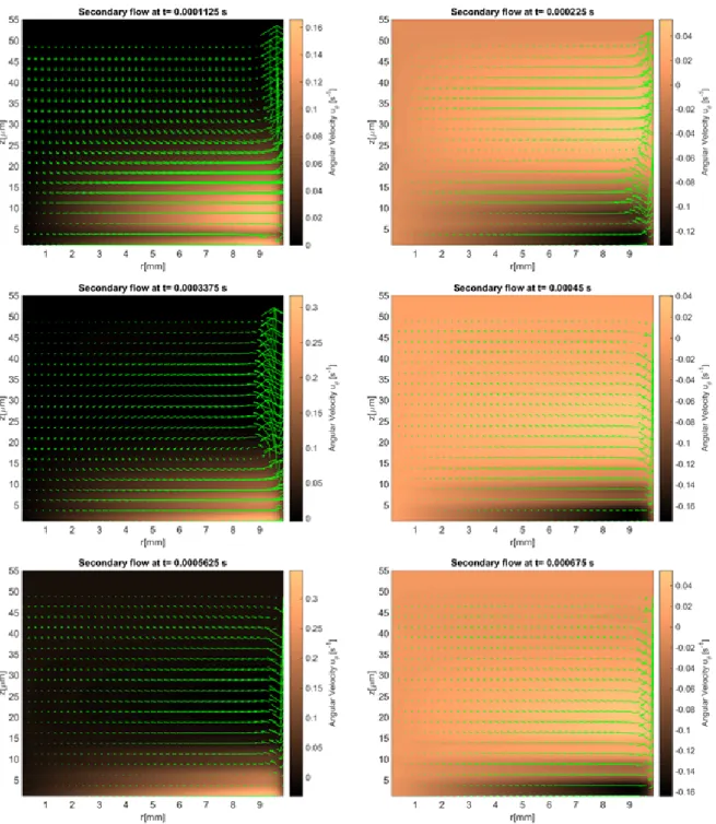
In Figure 2.11, we show the development of secondary flow patterns at various times at the
beginning stages of the swirling flow for Newtonian fluid. Here secondary flow refers to the (ur, uz)
components of the velocity field, sinceuθ is the primary velocity component for a rotational flow.
At early times, an outward centrifugal force causes the fluid near the rotating disk to flow radially
outward, up the sidewalls of the cylinder, inward along the top, and finally down near the center. A
vortex is formed here. After a certain amount of time, the flow will reach a quasi-steady state.
The same type of flow is shown for viscoelastic fluids in Figure 2.12, Figure 2.13 and Figure 2.14.
At early times, the secondary flow pattern and vortex is similar to those in Newtonian case. However,
with opposite orientation. This reverse orientation in the secondary flow is a classical consequence
of the generation of normal stresses in viscoelastic fluids; a property shared in all our viscoelastic
models. In the quasi-steady state of viscoelastic fluids, the fluid near the rotating disk flows radially
inward, up the center of the cylinder, inward along the top, and finally down near the sidewalls. In
stark contrast, for Newtonian fluids, the flow near the center is downward while upward near the
wall (Figure 2.16). This phenomenon has been long recognized in swirling cylindrical flow, called
the so-called Quelleffeck [5], an analog of the Weissenberg effect of rod climbing [5].
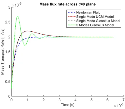
The mass flux rate across the θ= 0 plane for all the studied fluids is shown in Figure 2.17. For
Newtonian fluids the mass flux is increasing during the transients and eventually reaches a plateau
in steady state. However, for single-mode Giesekus and UCM model fluids, in the early transient
the mass flux rate first increases similar to the Newtonian flow, then decreases monotonically while
converging to steady state. The maximum mass flux rate arises during the formation of the reverse
vortex at the bottom corner of the cell culture. For the 5-mode Giesekus model, the transient mass
flux rate is non-monotone reflecting the effects of having more than one relaxation modes. Since
each fluid model has finite memory, the stationary mass transport rates are identical, irrespective
of the differences in secondary flow patterns. Thus there is no enhancement of mass transport for
unidirectional swirling flow due to viscoelasticity at steady state.
2.6.2 Numerical Mucus Flow in Cell Culture
In this section, we conduct the numerical simulation for the mucus flow in HBE cell culture. We
use the 5-modes Giesekus model from Section 2.3 as our constitutive model for mucus. And the
cilia driving condition is modeled as a piece-wise sinusoidal angular velocity functionf(t) at the
bottom plate given by
f(t) =
P0sin(ωpt), f or 0< t < ωπp
R0sin(ωrt), f or0< t < ωπp +ωπr
where P0 = 1.57×10⁻²s−1,R0= 7.9×10⁻³s−1,ωp= 10πHz andωp= 10πHz[Section 2.4].
We first examine the secondary flow profiles in Figure 2.18. As before, the early transient
Figure 2.13: Transient process of the flow field for a single mode Giesekus fluid withα= 0.3; the velocity field in the plot is the secondary flow (ur vs uz) and the color map in the background is
Figure 2.14: Transient process of the flow field for a 5 modes Giesekus fluid with parameters specified in Table 2.3; the velocity field in the plot is the secondary flow (ur vs uz) and the color map in the
Figure 2.15: The stationary secondary flow field and streamlines for nonlinear viscoelastic mucus model in the middle of the cell culture (left) and at the edge of the cell culture (right).
Figure 2.17: Mass transport flux rate across the θ= 0 plane for the swirling flow with different types of fluids
creating a downward flow near the wall and upward flow at the center of the culture. The mass flux
rate across theθ= 0 plane is shown in Figure 2.19 for all four constitutive models (viscous, 1-mode
UCM, 1-mode Giesekus, 5-mode Giesekus), with the result that after differences due to transients ,
they all converge to the same bulk flow rate for the pulsatile lower plate driving condition.
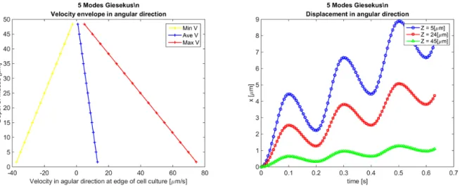
Next in Figure 2.20, we analyze the primary flow field, uθ, in particular, the envelopes of uθ
across the gap, as well as the displacement time series at the edge of the cell culture at different
heights. The resulting envelopes of the velocity exhibit a linear dependence across the gap. It can be
shown that the shear strain and shear rate envelopes across the gap are also linear, corresponding to
the so-called gap loading limit that is designed and exploited in rotational rheometers [26] [7]. We
note that this gap loading behavior holds for this current set of parameters, and we return below to
explore conditions that induce nonlinear primary flow behavior and departures from the gap-loading
Figure 2.19: Mass transport flux rate across one θ= 0 plane with oscillatory driving condition for 5 modes Giesekus fluid with parameters specified in Table 2.3;
2.7 Large Amplitude Oscillatory Shear(LAOS) Analysis of Nonlinearity
The linear primary flow profiles and shear strain and shear rate envelopes from the last section
imply two things: the flow conditions fall within the gap-loading regime and the driving conditions
induce a linear viscoelastic response, i.e., steady state results from Giesekus models overlap with
those of the UCM model. However, to rigorously assess the linear or nonlinear regime for the given
driving conditions, the standard procedure is to impose a sinusoidal shear strain at the bottom
plate, rather than the angular velocity boundary condition of our simulations thus far. Then one
checks for higher harmonic generation in the flow field [12] [4] [6]. The oscillatory driving condition
at the bottom of the cell culture for uθ does not imply a sinusoidal shear strain. Therefore, we
calculate the driving condition foruθ that is equivalent to an imposed sinusoidal shear strain.
imposed shear strain at bottom plate =γ0sin(ωt)
imposed shear rate=γ0ωcos(ωt)
shear rate= 1 2(
∂uθ
∂r − uθ
r )
uθ(r, z, t)|z=0 =C·r+ 2γ0ωcos(ωt)·r·log(r), C is a constant (2.1)
where C is an arbitrary constant. With the aboveuθ that results in a sinusoidal driving shear strain,
we can apply the standard nonlinear (Fourier) viscoelastic metrics for large amplitude oscillatory
shear [12].
We choose a set of parameters for the equation above such that the theta-component of the
velocity resembles the conditions imposed in the previous section, as illustrated in Figure 2.21.
We calculate the Fourier decomposition of the resulting shear strain, shear rate and shear
stress. We found that there are no higher harmonics greater than 3% of the fundamental harmonic.
Furthermore, everywhere in the cell culture, the shear strain is a sine function and the shear rate is
a cosine function. Figure 2.22 shows the envelopes of shear strain and shear stress across the height
of the cell culture at radius r = 0.5R.
Figure 2.23 shows the normalized Lissajous curves at different locations of our cell culture.
show the oscillatory stress as a parametric function of the strain, whereas viscous Lissajous curves
show the stress against the rate of strain. In this way, for an elastic solid, the elastic Lissajous
curves are represented by straight lines and viscous Lissajous curves by circles, while the opposite is
true for a viscous fluid. In the small amplitude regime for a generic viscoelastic fluid, both elastic
and viscous Lissajous curves are ellipses. Any departure from a perfect ellipse signals that the
nonlinear LAOS regime has been reached.
Figure 2.21: Left: Driving condition for uθ where uθ is a sinusoidal function of time; Right: Driving
condition for uθ where shear strain is a sinusoidal function of time
These results imply that, with the prescribed magnitude of the imposed angular velocity, the
solution resides in the gap-loading and the linear regime of the viscoelastic model. Since we are in
the linear regime, we can characterize the viscoelasticity of the mucus flow by calculating the linear
storage modulus G0, and loss modulus G0, versus position in the culture [Figure 2.24].
Next, we explore the implications relative to linear and nonlinear flow when the mucus ”hurricane”
is localized in the middle of the cell culture and does not extend all the way to the culture wall.
The effective radius of mucus flow is therefore smaller than the cell culture radius R=10mm. In the
next simulation, we set the effective radius of the mucus flow as 5mm instead of 10mm and change
the magnitude of the oscillatory driving velocity accordingly to match the experimental observation.
Figure 2.25 shows the envelopes of shear strain and shear stress across the height of the cell culture
Figure 2.22: The envelopes of shear strain(left) and shear stress(right) across the gap atr = 0.5∗R
Figure 2.24: Storage ModulusG0 (Left) and Loss ModulusG00 (Right) everywhere in the cell culture
no longer scale linearly and the shear stress is not constant across the gap, Figure 2.26 indicates that
for these conditions, the system is no longer in the gap-loading limit. The next step is to determine
whether or not the model response is linear or nonlinear. Figure 2.26 shows LAOS analysis results at
r=0.4*R and h=0.4*H, where the Lissajous curves now show a nonlinear response. These nonlinear
response can be quantified by means of the stress decomposition [4] and Chebyshev expansion [6].
For oscillatory shear with an imposed sinusoidal strain, the resultant stress can be decomposed into
elastic and viscous stresses by using symmetry arguments [4]. Ewoldt and McKinley suggested an
orthogonal decomposition of the elastic and viscous stresses using Chebyshev polynomials [6]. The
signs of third harmonic Chebyshev coefficientse3 (elastic stress) and 3 (viscous stress) indicate the
nature of the elastic and viscous nonlinearities. For our data e3 <0 and3 >0 implying the local
mucus flow at this position in the culture is strain-softening and shear-thickening.
We now characterize nonlinearity of the mucus flow for reasonable ranges of cell culture parameters
with the 5-mode Giesekus mucus model with parameters in Table 2.3. Figure 2.27 shows the linear
and nonlinear regime for mucus flow with respect to the aspect ratio of the hurricane (radial extent
versus mucus depth) and mean driving velocityuθ at r=0.5*R. When the aspect ratio is less than
100 and the mean uθ is greater than 70 µm/s, the mucus transport resides in the nonlinear regime
. A similar characterization of nonlinear mucus response can be carried out versus constitutive
Figure 2.25: The envelopes of shear strain(left) and shear stress(right) across the gap atr = 0.5∗R with R= 5mm.
2.8 Advection-diffusion of Drug Concentrations
In this section, we consider the scenario when an initial concentration of drug (or dye) is dropped at
the surface of the mucus layer, which besides being transported by the underlying velocity field, it
can diffuses freely in the HBE cell culture. We assume the drug does not alter the mucus properties
or flow field and that there is no affinity between the mucus gel network and the diffusing particles.
We further assume that the PCL-mucus interface absorbs any drug concentration that reaches it.
Finally, we use the flow fields obtained from our previous results using the 5-mode Giesekus model
from Table 1 and the cilia driving condition in Section 2.4.
For a drug concentrationC with constant diffusion coefficientD, the transport ofC inside the
mucus flow can be describe by the following advection-diffusion equation
∂C
∂t =D∆(C)− ∇ ·(uC) +S
whereS is the source of the concentration. Here we assume we have an initial concentration of C0
and no extra source, i.e. S= 0. In cylindrical form, the equation becomes
∂C ∂t =D[
1 r
∂ ∂r(r
∂C ∂r) +
1 r2
∂2C ∂θ2 +
∂2C ∂z2 ]−
ur
r ∂
∂r(rC)− uθ
r ∂C
∂θ −uz ∂C
We assume axisymmetry of the flow, but depending on the symmetry of the initial concentrationC0,
the advection-diffusion of C inside the cell culture might or might not be axisymmetric. However, if
C0 is axisymmetric, the concentration will remain so. In this case the advection-diffusion equation
reduces to
∂C ∂t =D[
1 r
∂ ∂r(r
∂C ∂r) +
∂2C ∂z2]−
ur
r ∂
∂r(rC)−uz ∂C
∂z
The boundary condition at the bottom plate is absorbing. The above equations are solved using
a finite different method. The unsteady velocity field is extracted from the stationary results in
Section 2.6.2.
Initially, a unit mass of drug is initially deposited in a small circular domain at the center of the
surface of the cell culture, that is we setC0 to be a disk of unit concentration with radius 0.1 mm
at the center of the air-mucus interface. Figure 2.28 depicts the surface of the cell culture and the
red dot is the domain of initial uniform concentration of the drug.
Figure 2.28: Initial drug concentration type 1; Blue disk shows the surface of the cell culture; red disk is the initial concentration of unit drug at the surface.
Using this initial condition, we investigate the effect of the diffusion coefficient on the distribution
of advection relative to diffusion,
P e= advective transport rate dif f usive transport rate =
L·V D
where L is the characteristic length, which is our case is 1×10⁻²m (length of the radius), V is the
characteristic flow velocity, which is our case is 1×10⁻⁹m/s (mean local velocity in the r direction,
note the mean local velocity in the θdirection is 1×10⁻⁴m/s). The diffusion coefficientDthat I
used here ranges from 1×10−15,1×10−14,· · ·,1×10−8,1×10⁻⁷ m2/s. Therefore the corresponding
Pe are 1×10⁻⁴, 1×10⁻³, 1×10⁻², 1×10⁻¹, 1, 1×10², 1×10³, 1×10⁴.
Figure 2.29 and Figure 2.30 shows the advection-diffusion process for the drug concentration
with P e= 0.1 and P e= 10 under the initial condition in Figure 2.28. Note that those figures are
plotted in a reduced 2D rectangle because of the axisymmetric assumption, see Figure 2.6 for details.
And as we can see from those plots, it seems like the drug is primarily diffusing in the z direction,
but not in the r direction. This perception is incorrect. It only looks this way because of the large
aspect-ratio we have for the HBE cell culture (10mmlength of radius and 50µmdepth of mucus
give us an aspect-ratio of 200). Therefore, with this large aspect-ratio and initial condition, most of
the drug would be absorbed by the bottom plate long before it makes any significant transport in
the radial direction.
Figure 2.31 shows the percentage of the drug concentration absorbed at the bottom plate by the
exterior domain to the initial circle of drug concentration. When Pe is small (D is large), almost
no drug will be absorbed on the outer part of the bottom plate . Since the drug primarily diffuses
in the z direction because of the large aspect-ratio (10 mm radius, 50µm depth, or aspect ratio
of 200). Therefore, with this large aspect ratio and initial condition, most of the drug would be
absorbed in a slightly larger radius domain at the bottom plate, with minimal radial diffusion and
minimal influence of advection by the mucus flow. Even when P e= 1×10⁴ (D= 1×10⁻¹⁵m2/s ),
only 5.2% of the drug concentration is absorbed by the outer part” of the bottom plate. Hence the
effect of mucus flow on the absorption of the drug concentration is minimal under these conditions.
Figure 2.31 shows the time it takes for 95% of the drug concentration to be absorbed by the outer
part of the bottom plate as a function ofP e.
Figure 2.31: The percentages of the drug concentration absorbed by outer part” of the bottom plate in the end versus Peclet number P e
culture, the initial drop in Figure 2.28 would not result in our goal. We could instead initially
spread the drug evenly on the entire surface of the mucus flow. Or more efficiently, we could take
advantage of mucus ”hurricane”, and drop the drug along a radius withθ= 0 of the surface of the
mucus flow, see Figure 2.33.
Next we explore different domains of deposition of the drug at the air-mucus interface (Figure
2.33). To quantify absorption across the different initial conditions, we measure the percentage of
the drug absorbed by a fan in the bottom plate with −π
12 < θ <
π
12, as illustrated in Figure 2.34.
This part takes up 121 (or 8.33%) portion of the entire bottom disk and is in the opposite direction
as the initial distribution of drug. If the drug is evenly absorbed by the bottom plate, this fan area
would absorb 8.33% of the total drug concentration. The closer the percentage absorbed by this fan
area is to 8.33%, the more effective the influence of advection. Figure 2.35 shows the result of the
percentage of drug concentration absorbed by the fan area in the bottom plate versus Peclet number.
We can see when P e <0.1, the drug transport is not effective; whenP e >1, the drug transport is
effective and whenP e >102, the drug transport is extremely effective since the percentage is quite
close to the ”perfect” score of 8.33%.
Figure 2.34: Initial drug concentration type 1; Blue disk shows the bottom of the cell culture; the red fan stands for the area where−π
12 < θ <
π
12.
2.9 Validating the Numerical Methods
The numerical methods we use here are adopted from [24]. Marker and Cell (MAC) method [20]
is used here to track the movement of the free surface. In the MAC method, artificial massless
trackers are placed near the free surface and are transported according to the fluid velocity. Cells
are flagged as fluid cells, surface cells and empty cells based on the location of all markers. Those
markers are able to track the free surface movement. A second order finite difference method is
used to discretized the space derivative on a staggered grid. Forward Euler scheme is used here for
the time integration.
2.9.1 Convergence
In the following test, we use 4 different sizes of grids (30 by 30, 40 by 40, 50 by 50 and 60 by 60)
to calculate the flow field and free surface shape of the swirling flow (constant angular driving
velocity) of the same singe mode UCM fluid, with We=1.0. After the flow reaches quasi-steady
state, we check the free surface shapes and the velocity field at the middle height of the cylinder to
see whether the numerical results converges or not.
The following four figures [Figure 2.36 to 2.39] show the results. From [Figure 2.36 to 2.38]
about the velocities components, it’s easy to see that the code converges as the grid gets finer. And
last figure [Figure 2.39] about the free surface suggests that the free surface curve also converges,
but with a slower rate.
2.9.2 Benchmarking
Here we first compare the evolution of the tangential velocities [Figure 2.40] after the stop of
the rotating disk with the result [Figure 14] from [27]. Then we compare the tangential velocity
distribution for a single mode UCM fluid after stabilization [Figure 2.41], with the result [Figure 6]
from [27]. By looking at Figure 2.40 and 2.41, we can see that the result for tangential velocity
distribution from our numerical method matches the result from [27] [Figure 6 and 14]. This should
suggest that our numerical algorithm is correct.
As we have seen in Section 2.6.1, one significant difference between viscoelastic fluid and
Figure 2.36: Convergence test: ur at the middle height for a single UCM fluid
Figure 2.38: Convergence test: uthetaat the middle height for a single UCM fluid
Figure 2.40: The evolution of the tangential velocities after the stop of the rotating disk for a single mode UCM fluid
surface of the viscoelastic fluid flows upwards along the axisymmetric swirling axis, rather than
downwards as in the case of Newtonian fluid. Its like rod-climbing without a rod. And a bulge is
generated at the upper surface of the fluid, which can be characterized by its vertical displacement
along the axis of symmetry as illustrated in Figure2.42.
Figure 2.42: Illustration of Quelleffekt
In [5], Debbaut and Hocq studied the relationship between the displacement h (displacement
in z-direction at the middle of the surface) and H (initial free surface height). In their numerical
experiment they used Johnson-Segalman model to model a 2.5% aqueous polyacrylamide solution.
Here I did the similar experiment with a single mode Giesekus fluid withα= 0.3, and plot the same
type of results that Debbaut and Hocq had for Johnson-Segalman model in [5]. Although exact
match is not possible here, we focused on the trend and qualitative matching between our results
and their results. In Figure 2.43 cited from [5], Debbaut and Hocq plot the free surface shape for
various values of H and the displacement h of the upper surface along the axis of symmetry as a
function of H for Johnson-Segalman model. In Figure 2.44 and 2.44, we plot the same figures but
with our algorithm for a single mode Giesekus fluid. By comparing our results in Figure 2.44 and
2.45 and their results in Figure 2.43, both the shape of free surface and the relation between the
displacement and initial surface height match with each other qualitatively. Given the fact that we
used a different fluid model from theirs and the overall trends are the same, I believe this partially
Figure 2.43: From [5]: free surface shapes for various H (a); Displacement h of the upper surface along the axis of symmetry as a function of H (b). Both for Johnson-Segalman model to model a 2.5% aqueous polyacrylamide solution.
CHAPTER 3
CONCLUSIONS
These are the first steps toward mucus flow in HBE cell culture simulations, with an idealized
coarse-graining of the cilia forcing condition. First, we clearly show nonlinear viscoelasticity captures
the simplest of observations: normal stress generation in shear leads to the peak of the free surface
in the middle of the culture and a depression at the walls, and the corresponding flow profile is
consistent with these free surface observations. Second, we characterized the linear and nonlinear
viscoelastic regimes versus the radius and mean rotational velocity of the mucus ”hurricane”; and
designed viscoelastic metrics to study the property of mucus across the whole cell culture. Third,
we examined the advection-diffusion process of a drug concentration dropped at the surface of the
mucus flow against different drug diffusion coefficient. The absorption of the drug by the bottom
plate of the cell cultures is explored for different initial concentrations and diffusion coefficient. And
we illustrated the ”flaw” of the absorption due to the large aspect-ratio and showed how to improve
the effectiveness of the absorption. The future work includes the generalization of the code to 3D
and extend the cilia forcing boundary conditions to experimentally measured metachronal wave
REFERENCES
[1] J. B. Bell, P. Colella, and H. M. Glaz. A second-order projection method for the incompressible navier-stokes equations. Journal of Computational Physics, 85(2):257–283, 1989.
[2] B. Button, L.-H. Cai, C. Ehre, M. Kesimer, D. B. Hill, J. K. Sheehan, R. C. Boucher, and M. Rubinstein. A periciliary brush promotes the lung health by separating the mucus layer from airway epithelia. Science, 337(6097):937–941, 2012.
[3] R. K. Chhetri, R. L. Blackmon, W.-C. Wu, D. B. Hill, B. Button, P. Casbas-Hernandez, M. A. Troester, J. B. Tracy, and A. L. Oldenburg. Probing biological nanotopology via diffusion of weakly constrained plasmonic nanorods with optical coherence tomography. Proceedings of the National Academy of Sciences, 111(41):E4289–E4297, 2014.
[4] K. S. Cho, K. Hyun, K. H. Ahn, and S. J. Lee. A geometrical interpretation of large amplitude oscillatory shear response. Journal of Rheology (1978-present), 49(3):747–758, 2005.
[5] B. Debbaut and B. Hocq. On the numerical simulation of axisymmetric swirling flows of differential viscoelastic liquids: the rod climbing effect and the quelleffekt. Journal of non-newtonian fluid mechanics, 43(1):103–126, 1992.
[6] R. H. Ewoldt, A. Hosoi, and G. H. McKinley. New measures for characterizing nonlin-ear viscoelasticity in large amplitude oscillatory shnonlin-ear. Journal of Rheology (1978-present), 52(6):1427–1458, 2008.
[7] J. D. Ferry. Viscoelastic properties of polymers. John Wiley & Sons, 1980.
[8] H. Giesekus. A simple constitutive equation for polymer fluids based on the concept of deformation-dependent tensorial mobility.Journal of Non-Newtonian Fluid Mechanics, 11(1):69– 109, 1982.
[9] D. B. Hill and B. Button. Establishment of respiratory air–liquid interface cultures and their use in studying mucin production, secretion, and function. InMucins, pages 245–258. Springer, 2012.
[10] D. B. Hill, V. Swaminathan, A. Estes, J. Cribb, E. T. O’Brien, C. W. Davis, and R. Superfine. Force generation and dynamics of individual cilia under external loading. Biophysical journal, 98(1):57–66, 2010.
[11] D. B. Hill, P. A. Vasquez, J. Mellnik, S. A. McKinley, A. Vose, F. Mu, A. G. Henderson, S. H. Donaldson, N. E. Alexis, R. C. Boucher, et al. A biophysical basis for mucus solids concentration as a candidate biomarker for airways disease. PloS one, 9(2):e87681, 2014.
[12] K. Hyun, M. Wilhelm, C. O. Klein, K. S. Cho, J. G. Nam, K. H. Ahn, S. J. Lee, R. H. Ewoldt, and G. H. McKinley. A review of nonlinear oscillatory shear tests: Analysis and application of large amplitude oscillatory shear (laos). Progress in Polymer Science, 36(12):1697–1753, 2011.
[14] M. Kesimer, S. Kirkham, R. J. Pickles, A. G. Henderson, N. E. Alexis, G. DeMaria, D. Knight, D. J. Thornton, and J. K. Sheehan. Tracheobronchial air-liquid interface cell culture: a model for innate mucosal defense of the upper airways? American Journal of Physiology-Lung Cellular and Molecular Physiology, 296(1):L92–L100, 2009.
[15] R. G. Larson. The structure and rheology of complex fluids, volume 33. Oxford university press New York, 1999.
[16] J. F. Lechner, A. Haugen, I. A. McClendon, and E. W. Pettis. Clonal growth of normal adult human bronchial epithelial cells in a serum-free medium. In vitro, 18(7):633–642, 1982.
[17] A. E. Likhtman and R. S. Graham. Simple constitutive equation for linear polymer melts derived from molecular theory: Rolie–poly equation. Journal of Non-Newtonian Fluid Mechanics, 114(1):1–12, 2003.
[18] C. W. Macosko and R. G. Larson. Rheology: principles, measurements, and applications. 1994.
[19] H. Matsui, S. H. Randell, S. W. Peretti, C. W. Davis, and R. C. Boucher. Coordinated clearance of periciliary liquid and mucus from airway surfaces. Journal of Clinical Investigation, 102(6):1125, 1998.
[20] S. McKee, M. Tom´e, V. Ferreira, J. Cuminato, A. Castelo, F. Sousa, and N. Mangiavacchi. The mac method. Computers & Fluids, 37(8):907–930, 2008.
[21] A. L. Oldenburg, R. K. Chhetri, D. B. Hill, and B. Button. Monitoring airway mucus flow and ciliary activity with optical coherence tomography. Biomedical optics express, 3(9):1978–1992, 2012.
[22] W. Philippoff. Vibrational measurements with large amplitudes. Transactions of The Society of Rheology (1957-1977), 10(1):317–334, 1966.
[23] M. Sanderson and M. Sleigh. Ciliary activity of cultured rabbit tracheal epithelium: beat pattern and metachrony. Journal of Cell Science, 47(1):331–347, 1981.
[24] M. Tom´e, A. Castelo, J. Murakami, J. Cuminato, R. Minghim, M. Oliveira, N. Mangiavacchi, and S. McKee. Numerical simulation of axisymmetric free surface flows. Journal of Computational Physics, 157(2):441–472, 2000.
[25] P. A. Vasquez and M. G. Forest. Complex fluids and soft structures in the human body. In
Complex Fluids in Biological Systems, pages 53–110. Springer, 2015.
[26] P. A. Vasquez, Y. Jin, K. Vuong, D. B. Hill, and M. G. Forest. A new twist on stokes second problem: Partial penetration of nonlinearity in sheared viscoelastic layers. Journal of Non-Newtonian Fluid Mechanics, 196:36–50, 2013.


![Figure 2.5: Surface shape of an HBE cell culture shows the dome at the center [21]](https://thumb-us.123doks.com/thumbv2/123dok_us/8259127.2188158/21.918.214.712.597.816/figure-surface-shape-hbe-cell-culture-shows-center.webp)
![Figure 2.8: Movement of a single cilium: power stroke and recovery stroke. Data replotted from [23] and adapted from [10].](https://thumb-us.123doks.com/thumbv2/123dok_us/8259127.2188158/26.918.259.646.382.712/figure-movement-single-cilium-stroke-recovery-replotted-adapted.webp)