A Study of Face Embedding in Face Recognition

A STUDY OF FACE EMBEDDING IN FACE RECOGNITION

A Thesis presented to

the Faculty of California Polytechnic State University, San Luis Obispo

In Partial Fulfillment

of the Requirements for the Degree Master of Science in Computer Science

by Khanh Duc Le

COMMITTEE MEMBERSHIP

TITLE: A Study of Face Embedding in Face Recog-nition

AUTHOR: Khanh Duc Le

DATE SUBMITTED: March 2019

COMMITTEE CHAIR: Xiaozheng (Jane) Zhang, Ph.D. Professor of Electrical Engineering

COMMITTEE MEMBER: Foaad Khosmood, Ph.D. Professor of Computer Science

COMMITTEE MEMBER: Franz Kurfess, Ph.D.

ABSTRACT

A Study of Face Embedding in Face Recognition

Khanh Duc Le

Face Recognition has been a long-standing topic in computer vision and pattern recognition field because of its wide and important applications in our daily lives such as surveillance system, access control, and so on. The current modern face recognition model, which keeps only a couple of images per person in the database, can now recognize a face with high accuracy. Moreover, the model does not need to be retrained every time a new person is added to the database.

By using the face dataset from Digital Democracy, the thesis will explore the ca-pability of this model by comparing it with the standard convolutional neural network based on pose variations and training set sizes. First, we compare different types of pose to see their effect on the accuracy of the algorithm. Second, we train the sys-tem using different number of training images per person to see how many training samples are actually needed to maintain a reasonable accuracy.

ACKNOWLEDGMENTS

Thanks to:

• Mom and Dad for their constant support, love, and belief that I can accomplish whatever I set my mind to

• Professor Jane Zhang for kindling my love for computer vision and machine learning

• My friends, for their encouragement throughout my school year at Cal Poly

TABLE OF CONTENTS

Page

LIST OF TABLES . . . ix

LIST OF FIGURES . . . x

CHAPTER 1 Introduction . . . 1

2 Background . . . 4

2.1 History . . . 4

2.2 Neural Networks . . . 6

2.2.1 Overview . . . 6

2.2.2 Activation Functions . . . 7

2.2.2.1 ReLU . . . 7

2.2.3 Loss Function . . . 9

2.2.3.1 Hinge Loss . . . 9

2.2.3.2 Cross-Entropy Loss . . . 10

2.2.4 Optimization Methods . . . 10

2.2.4.1 Gradient Descent . . . 11

2.2.4.2 Stochastic Gradient Descent . . . 11

2.2.4.3 Stochastic Gradient Descent with Momentum . . . . 11

2.2.5 Backpropagation . . . 12

2.3 Convolutional Neural Network . . . 13

2.3.1 Convolutional Layers . . . 14

2.3.2 Activation Layers . . . 15

2.3.4 Fully-Connected Layers . . . 16

2.3.5 Batch Normalization . . . 16

2.3.6 Dropout . . . 17

2.4 Common Architectures . . . 19

2.4.1 VGGNet . . . 19

2.4.2 GoogLeNet . . . 20

2.5 Siamese Neural Network . . . 21

2.5.1 Siamese Network . . . 22

2.5.2 Triplet Loss Function . . . 22

2.6 Evaluation Metrics . . . 24

2.6.1 Accuracy . . . 24

2.6.2 Precision - Recall - F1 Score . . . 24

2.6.2.1 Precision . . . 25

2.6.2.2 Recall . . . 25

2.6.2.3 F1-Score . . . 25

3 Related Work . . . 26

3.1 Traditional Methods . . . 26

3.2 Deep Learning Methods . . . 27

3.2.1 Mainstream Architectures . . . 27

3.2.1.1 Special Architectures . . . 28

3.2.1.2 End-to-End Network . . . 28

4 Design and Implementation . . . 30

4.1 Tools . . . 30

4.1.1 Keras . . . 30

4.2 Dataset . . . 31

4.2.1 Training Machine . . . 32

4.3 Face Recognition Pipeline . . . 32

4.3.1 Split Dataset . . . 34

4.3.2 Building Image Dataset . . . 36

4.3.3 Baseline Network . . . 36

4.3.3.1 Siamese Network and Classifier . . . 38

5 Experiments and Results . . . 39

5.1 Training Baseline Network - VGGNet . . . 39

5.1.1 Experiment #1 . . . 39

5.1.2 Experiment #2 . . . 40

5.2 Experiment #1: The Effect of Pose Variations and Training Set Sizes 43 5.2.1 Experiment #1a - Pose Variations . . . 43

5.2.2 Experiment #1b - Mixing Different Poses . . . 46

5.3 Experiment #2 - Face Generation to Enrich the Dataset . . . 47

5.4 Experiment #3 - Improving the Model . . . 49

5.5 Experiment #4 - Amazon Rekognition . . . 51

5.6 Performance . . . 53

6 Conclusion . . . 55

7 Future Work . . . 56

7.1 Classification . . . 56

7.2 Face Generation . . . 56

7.3 Face Alignment . . . 57

LIST OF TABLES

Table Page

4.1 Splitting Proportion for Baseline Network . . . 35

4.2 Split Proportion for Siamese Network with Classifier . . . 36

5.1 VGGNet - Experiment 2 - Evaluation Table . . . 40

LIST OF FIGURES

Figure Page

2.1 XOR (Exclusive OR) Dataset . . . 5

2.2 A Simple Neural Network Architecture . . . 6

2.3 Visualization of Different Activation Functions . . . 8

2.4 An Example of CNN Architecture (Adapted from Le-Cun et al. [Y. A. LeCun, L. Bottou, G. B. Orr, and K.-R. M uller.]) . . . 14

2.5 Left: 2 Layers of Neural Network That Are Fully-Connected with No Dropout. Right: The Same 2 Layers After Dropping 50% of the Connections . . . 18

2.6 The Architectures of VGGNet and GoogLeNet (Adapted from M. Wang and W. Deng. [48]) . . . 19

2.7 Visualization of VGGNet [42] . . . 20

2.8 Visualization of Inception Module Used in GoogLeNet [46] . . . 21

2.9 Siamese Network [6] . . . 22

2.10 Triplet Loss Function . . . 23

3.1 Top Row: Standard Network Architectures in Deep Object Classi-fication. Bottom Row: Deep FR that Use Standard Architectures and Achieve Good Performance [47] . . . 27

4.1 Example of the HDF5 Data Structure. . . 31

4.2 Sample of Digital Democracy Face Dataset . . . 32

4.3 Top Row: Pose Variation Issue, Middle Row: Illumination Issue, Last 3 Rows: Mislabeled Faces Issue . . . 33

4.4 Example of the HDF5 Data Structure. . . 34

4.6 First 2 CONV Layers of MiniVGGNet. Each CONV Consists of

(CONV, ACT, BN) . . . 37

5.1 VGGNet - Experiment 1 . . . 39

5.2 VGGNet - Experiment 2 - Trained with SGD, Initial Learning Rate = 1e−3 _{. . . . 42}

5.3 Sample Frontal Images from Face Dataset . . . 43

5.4 Sample Down Images from Face Dataset . . . 44

5.5 Sample Side Images from Face Dataset . . . 44

5.6 Front-view Faces Dataset Sizes vs Accuracy . . . 45

5.7 Front-view Faces Dataset Sizes vs Accuracy . . . 46

5.8 Generated Faces from Different Classes Using Masi et al. Algorithm [31] . . . 48

5.9 Mix-view and Generated Dataset Sizes vs Accuracy . . . 49

Chapter 1 INTRODUCTION

Face recognition is an important research topic in computer vision and pattern recognition field because it has a wide range of applications to daily lives such as surveillance system, access control, law enforcement, and so on.

Traditional methods attempted to solve face recognition problem by using hand-crafted features such as Fisher vector [12], Local Binary Pattern [34] and combining it with a classifier such as Support Vector Machine [10] to recognize the face. Currently, deep learning methods, especially Convolutional Neural Network (CNN), has proven to be more effective in face recognition against the traditional methods because the features are automatically learned from the training process itself [24]. Moreover, since the network is organized into many layers, it is able to learn multiple levels of representations that correspond to different levels of abstraction. The levels form a hierarchy of concepts, showing strong invariance to the face pose, lighting, and expression changes.

However, there still exists two major challenges in face recognition that a CNN cannot completely solve: (1) the ability to recognize a person by just feeding one picture of that his face into the system, and (2) the need not to retrain the model every time a picture of a new face is added to the system.

classifica-tion problem whose inputs are embedding vectors instead of face images. This leads us to three research questions:

1. Does the embedding vectors are discriminative enough to perform well on an-other completely different dataset?

2. How many training samples are enough to achieve a reasonable accuracy? 3. What can we do to reduce the training samples to imitate the real-life situation,

where we can only access to one or two face images for each person at most?

This thesis will explore the pros and cons of the current face recognition system by comparing it with the standard neural network based on different criteria such as pose variations and number of training images for classification. To do that, we use the face dataset from Digital Democracy. Digital Democracy is a project managed by the Institute for Advanced Technology and Public Policy at California Polytechnic State University, San Luis Obispo. It creates and provides a platform where anyone can search, watch, and share statements made by state lawmakers, lobbyists and advocates as they testify, debate, craft, and vote on policy proposals. Therefore, the dataset contains a lot of face images from different state legislative committee. We dive deeper into the study of embedding vectors to assemble the following list of contributions:

1. Create a standard convolutional neural network VGGNet, which acts as a base-line network for the experiments.

2. Collect the pose dataset. Each person has 3 types of poses: front-view, side-view, and down-view pose, each pose has 20 images in total.

with the number of training samples ranging from 1 up to 20 images per person.

4. Integrate a face generation technique with the classifier to increase the dataset sizes, thus reducing the actual number of face images needed per person

Chapter 2 BACKGROUND

2.1 History

Neural networks and deep learning have been around since the 1940s, going by different names based on various popular research trends at a given time, includ-ing cybernetics, connectionism, and the most familiar, Artificial Neural Networks (ANNs).

The first neural network model came from McCuloc and Pitts in 1943 [39]. This network was a binary classifier, capable of recognizing two different categories based on some input. The problem was that the weights used to determine the class label for a given input needed to be manually tuned by a human.

Then, in the 1950s, the Perceptron algorithm was published by Rosenblatt [37] -this model could automatically learn the weights required to classify an input without human intervention. The procedure to automatically train the perceptron formed the basis of Stochastic Gradient Descent (SGD) which is still used to train very deep neural networks today.

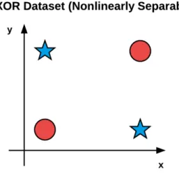
However, a 1969 publication by Minsky and Papert [31] stagnated neural network research for nearly a decade. Their work demonstrated that a Perceptron with a linear activation function was merely a linear classifier and unable to solve nonlinear problems. An example of nonlinearly separable function is the XOR problem (Figure 2.1):

Figure 2.1: XOR (Exclusive OR) Dataset

research in the backpropagation algorithm enables multi-layer feedforward neural networks to be trained. Combined with nonlinear activation functions, researchers could now solve nonlinear problems. Although the backpropagation algorithm is the cornerstone of modern neural network, at that time, due to slow computers and lack of large labeled training sets, researchers were unable to train neural networks that had more than two hidden layers.

Today, the latest incarnation of neural networks is called deep learning. What sets deep learning apart from its previous incarnations is that there is faster and specialized hardware with more available training data. Networks now can be trained with many more hidden layers that are capable of hierarchical learning where simple concepts are learned in the lower layers and more abstract patterns in the higher layers of the network.

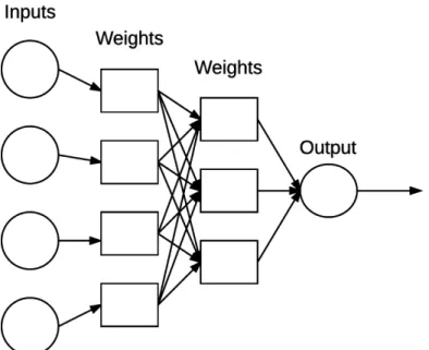
Figure 2.2: A Simple Neural Network Architecture

and corners to learn more abstract concepts useful for discriminating between image classes. In many applications, CNNs are now considered the most powerful image classifier and are currently responsible for pushing the state-of-the-art forward in computer vision and machine learning. In the next two sections, the background in neural network and CNN basics will be introduced.

2.2 Neural Networks

2.2.1 Overview

Neural networks are the building blocks of deep learning systems. A neural net-work contains a labeled, directed graph structure where each node in the graph per-forms some simple computation. A directed graph consists of a set of nodes (i.e., vertices) and a set of connections (i.e., edges) that link together pairs of nodes. An example of a neural network is shown in Figure 2.2.

be vectors used to quantify the contents of an image such color histograms, Histogram of Oriented Gradients [11], Local Binary Patterns [8], and so on. In the context of deep learning, these inputs are the raw pixel intensities of the images themselves.

Eachxis connected to a neuron via a weight vectorW consisting ofw1, w2, ...wn, meaning that for each inputx we also have an associated weight w.

Finally, the output node on the right of Figure 2.2 takes the weighted sum, applies an activation function f, which is discussed in the next section, and outputs a value. The output can be expressed as following:

f(w1x1+w2x2+...+wnxn) or

f(net) wherenet=w1x1+w2x2+...+wnxn

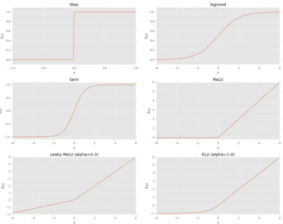
2.2.2 Activation Functions

An activation function is the function that decides whether a neuron should be activated or not. The activation function does the non-linear transformation to the input before sending it to the next layer of neurons, thus making it capable to learn and perform more complex tasks. There are a lot of activation functions (Figure 2.3), but we only use the ReLU in the thesis.

2.2.2.1 ReLU

ReLU [15], which stands for Rectified Linear Unit, is the most widely used acti-vation function in deep learning:

f(net) =max(0, net)

Figure 2.3: Visualization of Different Activation Functions

arises when we have a value of zero - the gradient cannot be taken.

To improve the classification accuracy, we need to tune, or learn, the parameters of the weight matrix W and bias vector b. To do that, two following important concepts will be discussed:

1. Loss functions

2. Optimization methods

2.2.3 Loss Function

A loss function quantifies how well the predicted class labels agree with the ground-truth labels. The smaller the loss, the better a job the classifier is at modeling the relationship between the input data and output class labels. Therefore, the goal when training the neural network is to minimize the loss function, thereby increasing the classification accuracy.

2.2.3.1 Hinge Loss

This is the loss that is inspired by (Linear) Support Vector Machines (SVMs) classifier [10], which uses an scoring function f to map the data points to numerical scores for each class labels. This functionf is a simple learning mapping:

f(xi, W, b) = W xi+b

To determine how good or bad this function is (given the weight matrixW and bias vector b) at making predictions, a loss function comes into play:

Li =X j6=yi

max(0, sj −syi + 1)

where sj is the predicted score of the j-class via the i-th data point: sj =f(xi, W)j. Essentially, this loss function sums across all incorrect classes (i 6=j) and compares the output of the scoring function s returned for the j-th class label (the incorrect class) and the yi-th class (the correct class). The max operation is applied to clamp the values at zero; thus ensuring we do not sum negative values. If the loss is zero -this implies that the class is correctly predicted. If the loss function is greater than zero, it means the prediction is incorrect.

individualLi:

L= 1 N

N X

i=1 Li

2.2.3.2 Cross-Entropy Loss

In the context of deep learning, the cross-entropy loss is more popular than the hinge loss function. Unlike the hinge loss function that treats the outputsf(xi, W) as uncalibrated scores for each class, cross-entropy loss, which comes from the Softmax classifier, gives more intuitive output because it returns the probabilities for each class. Probabilities are much easier for humans to interpret, so this fact is a particularly nice quality of cross-entropy loss.

Li =−log

es_yi P

jesyi !

The actual exponentiation and normalization via the sum of exponents inside the log bracket is the Softmax function. In general, it takes a vector of arbitrary real-valued scores and squashes it to a vector of values between zero and one that sum to one. The negative log of this function yields the actual cross-entropy loss.

Just as in hinge loss, computing the cross-entropy loss over an entire dataset is done by taking the average:

L= 1 N

N X

i=1 Li

2.2.4 Optimization Methods

Obtaining a high accuracy classifier is dependent on finding a set of weights W

2.2.4.1 Gradient Descent

The gradient descent method is an iterative optimization algorithm that operates over a loss landscape (also called an optimization surface). Each position along the surface corresponds to a particular loss value given a set of parameters W and b. The goal is to try different values of W and b, evaluate their loss, and then take a step towards better values that have lower loss.

2.2.4.2 Stochastic Gradient Descent

Stochastic Gradient Descent (SGD) is a simple modification to the standard gra-dient descent algorithm. It computes the gragra-dient and updates the weight matrix

W on small batches of training data, rather than the entire training set. While this modification leads to more noisy updates, it also allows us to take more steps along the gradient (one step per each batch versus one step per epoch), ultimately leading to faster convergence and no negative effects to loss and classification accuracy. The formula can be expressed as follows:

Wt+1 =Wt−α∇f(Wt)

whereαis the learning rate,∇f(Wt) is the gradient (or derivative) of the loss function with respect to W.

2.2.4.3 Stochastic Gradient Descent with Momentum

This is an extension of SGD that uses momentum [37], a method used to accelerate SGD, enabling it to learn faster by focusing on dimensions whose gradient point in the same direction. Momentum introduces a velocity term and utilizes it to calculate smoother gradients:

W =W −αvt+1

wherev is the velocity and γ is the momentum coefficient. γ is commonly set to 0.9; although another common practice is to setγ to 0.5 until learning stabilizes and then increase it to 0.9 [36]

To sum up, the input will pass through the neural network from input layer to the output layer. For each layer, it calculates the weighted sum of the input x and weights w. Then, an activation function is applied to this weighted sum, and then the results are passed through the next layer. Finally, at the end of the network, the loss function is used to calculate the total error between the predicted results and the actual results. To minimize the total error, optimization algorithms (i.e., SGD) are used to find the minima of the loss function. However, using the gradient descent in neural network is not an easy task because the neural network consists of multiple layers, each layer contains multiple neurons and are connected to each other by the weights. That is the reason the concept of backpropagation comes into play.

2.2.5 Backpropagation

Backpropagation is an efficient technique to perform gradient descent in neural networks [39]. In general, we calculate the gradient for a given layer by using the incoming gradient from the layer above us and the activations and weights at that layer; which follows from the chain rule. This algorithm is called backpropagation because a given layer0s gradient depends on the layer above it and the gradients are being passed backwards through the net. Once all the gradients from all the layers are calculated, we perform the normal gradient step as in any other gradient descent methods.

The backpropagation algorithm consists of two phases:

network and output predictions obtained

2. The backward pass (weight update phase) where the gradient of the loss function is computed at the final layer (i.e., predictions layer) of the network and used to recursively apply the chain rule to update the weights in our network.

Unfortunately, standard neural networks fail to obtain high classification accuracy when working with challenging image datasets that exhibit variations in translation, rotation, viewpoint, etc. In order to obtain reasonable accuracy on these datasets, Convolutional Neural Networks, a special type of feedforward neural networks, must be used.

2.3 Convolutional Neural Network

The convolutional neural network (CNN) is an evolution of the multi-layer neural network [24]. CNNs are built by stacking a sequence of layers where each layer is responsible for a given task. Convolutional layers learn a set of convolutional filters. Activation layers are applied on top of the convolutional layers to obtain a nonlinear transformation. Pooling layers help reducing the spatial dimensions of the input volume as it flows through the network. Once the input volume is sufficiently small, fully-connected layers are applied as the very last layers for the final output predictions. These layers are fully discussed in the following sub sections.

In practice, CNNs give two key benefits: local invariance and compositionality.

composition allows the network to learn richer features deeper in the network. For example, the network can build edges from pixels, shapes from edges, and then com-plex objects from shapes - all in an automated way that happens naturally during the training process. The concept of building higher-level features from lower-level ones is exactly why CNNs are so powerful in computer vision.

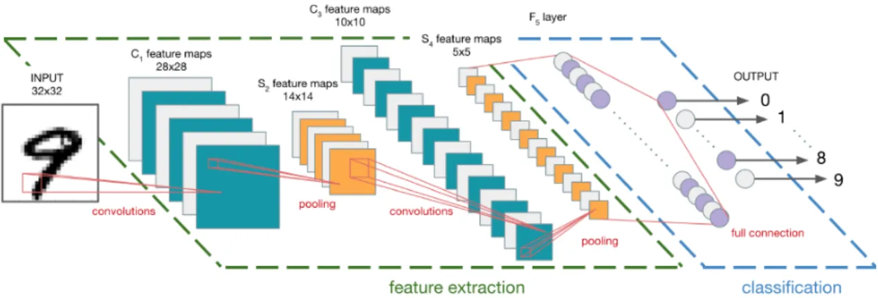
The following subsections describe various types of layers to build the CNN fol-lowed by a deeper discussion of CNN architecture designed for face recognition. Figure 2.1 illustrates an example architecture of a CNN to classify handwritten digits from the MNIST dataset [24]:

Figure 2.4: An Example of CNN Architecture (Adapted from Le-Cun et al. [Y. A. LeCun, L. Bottou, G. B. Orr, and K.-R. M uller.])

2.3.1 Convolutional Layers

The convolutional (CONV) layer is the core building block of a CNN. The CONV layer parameters consist of a set of K learnable filters where each filter has a width and a height. These filters are small but extend throughout the full depth of the volume. For inputs to the CNN, the depth is the number of channels in the image, but for volumes deeper in the network, the depth is the number of filters applied in the previous layer.

height of the input volume. Each kernel produces an 2D output, called an activation map. After applying all K filters to the input volume, K 2-dimensional activation maps are created. ThoseK activation maps then are stack along the depth dimension of the array to form the final output volume.

There are three parameters that control the size of an output volume: thedepth, stride, and zero-padding

Depth: The depth of an output volume controls the number of neurons in the CONV layer that connect to a local region of the input volume

Stride: Stride controls how the filter convolves around the input volume. For example, if stride = 3, the filter convolves around the input volume by shifting three units at a time.

Zero-padding: Zero padding pads the input volume with zeros around the border such that output volume size matches the input volume size. Without zero padding, the spatial dimensions of the input volume will decrease too quickly, and training deep network becomes more difficult since the input volume will be too small to learn any useful patterns from.

2.3.2 Activation Layers

2.3.3 Pooling Layers

A pooling (POOL) layer is used to progressively reduce the spatial size (i.e., width and height) of an input volume. This can reduce the amount of parameters and computation in the network, which also helps control overfitting.

POOL layers operate on each of the depth slices of an input independently using either a max oraverage function. Max pooling is typically done in the middle of the CNN architecture to reduce spatial size, whereas average pooling is normally used as the final layer of the network (i.e., GoogLeNet) to avoid using fully-connected layer entirely.

2.3.4 Fully-Connected Layers

Neurons in fully-connected (FC) layers are fully-connected to all activations in the previous layer, which is similar to traditional neural networks. It is often used along with the softmax classifier, which will compute the final output probabilities for each class to predict which class the input belongs to.

2.3.5 Batch Normalization

Batch normalization (BN) layers are used to normalize the activations of a given input volume before passing it into the next layer in the network [22]. Ifx is the mini-batch of activations, the normalized ˆxcan be computed via the following equation:

ˆ xi =

xi−µβ q

σ2 β +ε

During training, the µβ and σβ over each mini-batchβ, where:

µβ = 1 m

m X

σ2_β = 1 m

m X

i=1

(xi−µβ)2

During testing, mini-batch µβ and σβ is replaced with running averages of µβ and σβ computed during the raining process. This ensures that images passing through the network still obtain accurate predictions without being biased by theµβ and σβ from the final mini-batch passed through the network at training time.

Batch normalization has been shown to be extremely effective at reducing the number of epochs it takes to train the neural network. Batch normalization also has the benefit of stabilizing the training process, allowing for a larger variety of learning rates and regularization strengths. Therefore, it can help to prevent overfitting and allows to obtain significantly higher classification accuracy in fewer epochs compared to the same network architecture without batch normalization.

2.3.6 Dropout

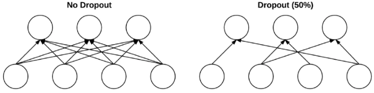
Dropout is actually a form of regularization that aims to help prevent overfitting by increasing testing accuracy, perhaps at the expense of training accuracy [20]. For each mini-batch in the training set, dropout layers, with probabilityp, randomly dis-connect inputs from the preceding layer to the next layer in the network architecture. Figure 2.2 visualizes this concept where some connections are randomly dropped with probability p= 0.5 between two FC layers for a given mini-batch:

The reason dropout reduces overfitting is that it explicitly alters the network architecture at training time. Randomly dropping connections ensures that no single node in the network is responsible for activating when presented with a given pattern. Instead, dropout ensures there are multiple, redundant nodes that will activate when presented with similar inputs - this helps the model to generalize better.

Figure 2.5: Left: 2 Layers of Neural Network That Are Fully-Connected with No Dropout. Right: The Same 2 Layers After Dropping 50% of the Connections

2.4 Common Architectures

(a) VGGNet

(b) GoogLeNet

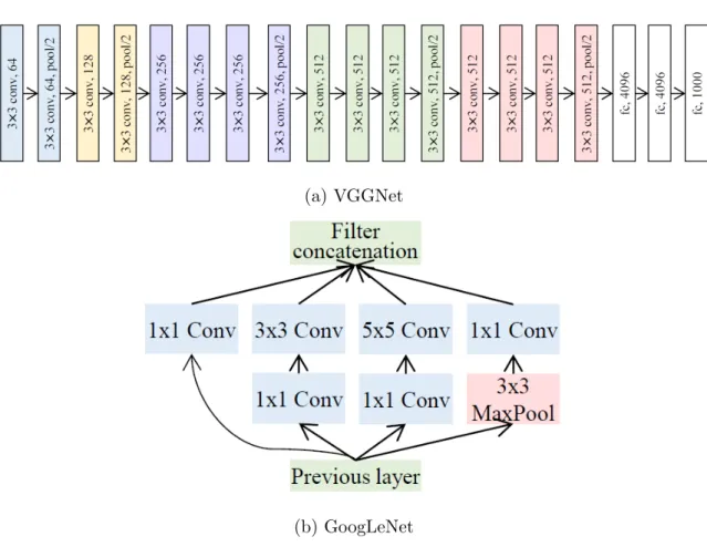
Figure 2.6: The Architectures of VGGNet and GoogLeNet (Adapted from M. Wang and W. Deng. [48])

2.4.1 VGGNet

The VGGNet (Figure 2.7) [42], which was introduced in 2014, is characterized by using only 3×3 convolutional layers stacked on top of each other in increasing depth. Reducing volume size is handled my max pooling. Two fully-connected layers each with 4096 nodes are then followed by a softmax classifier. The overall depth of the network is increased to 16-19 layers, which improve the ability to learn nonlinear mappings.

Figure 2.7: Visualization of VGGNet [42]

and the network weights themselves are quite large due to its depth and number of fully-connected nodes.

2.4.2 GoogLeNet

Modern state-of-the-art CNN utilize micro-architectures, also called network-in-network modules [26]. Micro-architectures are small building blocks where the output from one layer can split into a number of various paths and be rejoined later. This enables networks to learn faster and more efficiently since it can learn multiple things at the same time. These micro-architecture building blocks are stacked, along with conventional layer types such as convolutional layers, pooling layers, etc., to form the overall macro-architecture.

GoogLeNet introduces the Inception module [46], which is a micro-architecture that tries to learn convolutional layers with multiple filter sizes, turning the module into a multi-level feature extractor (Figure 2.8).

Figure 2.8: Visualization of Inception Module Used in GoogLeNet [46]

1×1 local features from the input. Thesecond branch first applies 1×1 convolution to reduce the dimensionality of the inputs before performing 1×1 convolution. By doing this, the amount of computation required by the network can be largely reduced.

The third branch applies the same logic as the second branch, but this time with the goal of learning 5×5 filters. Thefourth branch performs 3×3 max pooling with a stride of 1×1.

Finally, all four branches of the Inception module converge where they are con-catenated together along the channel dimension before being fed into the next layer in the network.

2.5 Siamese Neural Network

is created to overcome these problems.

2.5.1 Siamese Network

Siamese networks are a special type of neural network architecture [6]. Instead of a model learning to classify its inputs, the neural networks learns to differentiate between two inputs. Its objective is to find how similar two comparable things are. This network has two identical sub-networks, which both have the same parameters and weights. Each image in the image pair is fed to one of these networks. It then followed by a sequence of convolutional, pooling, fully connected layers and finally is fed to a triplet loss function (Figure 2.9).

Figure 2.9: Siamese Network [6]

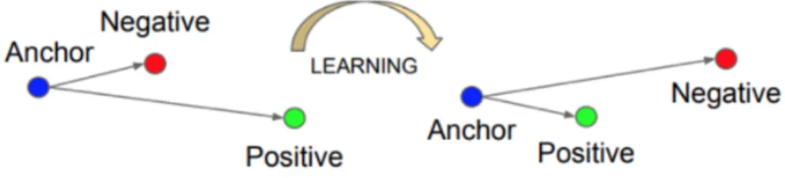
2.5.2 Triplet Loss Function

Figure 2.10: Triplet Loss Function

The loss function can be expressed in the following formula:

L=max(||f(xa

i)−f(x p i)||

2

2− ||f(x a

i)−f(x n i)||

2

2+α,0) wherexa

i,x p

i,xni are the anchor, positive, and negative samples, respectively;α is the margin, and f(.) represents a nonlinear transformation embedding an image into a feature space.

Finally, the neural network is trained using gradient descent on this cost function. To get better training results it is important to choose triplets that are hard to train on. If the triplet images are chosen randomly, it will be so easy to satisfy the constraint of the loss function because the distance is too large for most of the time. Therefore, the network will not learn much from the training set.

But once the network has been trained, it can generate embedding vector for any face, even the ones it has never seen before. In this thesis, we will use the pretrained model OpenFace of FaceNet [5] to extract embedding vectors and then compare with the baseline VGGNet.

2.6 Evaluation Metrics

2.6.1 Accuracy

Rank-1 accuracy is the percentage of predictions where the top prediction match the ground-truth label. This is the standard type of accuracy - the number of correct predictions are divided by the number of data points in the dataset.

Rank-5 accuracy is an extension of rank-1 accuracy: instead of caring about only the first prediction from he classifier, the top five predictions from the network are taken into account.

Computing rank-5 accuracy is redundant for small datasets, but for large, chal-lenging datasets, especially for the fine-grained classification, where the difference between categories are very subtle, it is helpful to look at the top-5 predictions from a given CNN to see how the network is performing.

Ideally, rank-1 accuracy would increase at the same rate as rank-5 accuracy. But on the challenging dataset, rank-5 accuracy is examined as well to ensure the network is still ”learning” in later epochs. It may be the case where rank-1 accuracy stagnates towards the end of training, but rank-5 accuracy continues to improve as the network learns more discriminating features, but not discriminative enough to overtake the rank-1 predictions.

2.6.2 Precision - Recall - F1 Score

2.6.2.1 Precision

P recision= T rueP ositive

T rueP ositive+F alseP ositive

Precision is the number of True Positives divided by the number of True Positives and False Positives. Precision can be thought of as a measure of a classifier0s exactness. A low precision can indicate a large number of False Positives

2.6.2.2 Recall

Recall= T rueP ositive

T rueP ositive+F alseN egative

Recall is the number of True Positives divided by the number of True Positives and the number of False Negatives. Recall can be thought of as a measure of a classifier0s completeness. A low recall indicates many False Negatives.

2.6.2.3 F1-Score

F1−score= 2× P recision×Recall P recision+Recall

Chapter 3 RELATED WORK

This chapter reviews some of the cornerstone studies that helped pushing forward the face recognition research.

3.1 Traditional Methods

Early face recognition system relied on facial landmarks extracted from images [13]. The method, which was introduced in 1971, proposes 21 subjective facial fea-tures, such as hair color and lip thickness, to identify a face in photograph. The largest drawback of this approach was that the 21 measurements are manually computed, therefore, it is highly subjective and prone to error.

3.2 Deep Learning Methods

3.2.1 Mainstream Architectures

When AlexNet won the ImageNet competition by a large margin using deep learn-ing in 2012 [23], research focus in face recognition shifted to deep-learnlearn-ing-based approaches. Unlike the traditional methods, which learn only one or two low-level representations as Eigenfaces for Fisherfaces, CNN learns multiple levels of represen-tations that correspond to different levels of abstraction. Those levels of abstraction overcome the challenges in FR such as illumination, pose, lighting, and expression changes. Some of the most influential network architectures that have shaped the cur-rent state-of-the-art of deep object classification and deep face recognition are shown in chronological order in Figure 3.1:

Figure 3.1: Top Row: Standard Network Architectures in Deep Object Classification. Bottom Row: Deep FR that Use Standard Architectures and Achieve Good Performance [47]

In 2015, FaceNet [41] used a large private dataset to train a GoogleNet. It adopted a triplet loss function based on triplets of roughly aligned matching/non-matching face patches generated by a novel online triplet mining method and achieved 99.63% on LFW dataset. In the same year, VGGface [35] designed a procedure to collect a large-scale dataset from the Internet. It trained the VGGNet on this dataset and then fine-tuned the networks via a triplet loss function similar to FaceNet. VGGface obtains an accuracy of 98.95% on LFW dataset.

In 2017, SphereFace [29] used a 64-layer ResNet architecture and proposed the angular softmax (A-Softmax) loss to learn discriminative face features with angular margin (99.42% on LFW).

3.2.1.1 Special Architectures

In addition, there are some special architectures in face recognition. Light CNN [51] proposed a max feature-map (MFM) activation function that introduces the concept of maxout in the fully connected layer to CNN. The MFM obtains a compact representation and reduces the computational cost. Inspired by bi-linear CNN model [27], Chowdhury et al applied bi-linear CNN (B-CNN) in face recognition [9]. The output at each location of two CNNs are combined using outer product and are then average pooled to obtain the bi-linear feature representation.

3.2.1.2 End-to-End Network

Chapter 4

DESIGN AND IMPLEMENTATION

4.1 Tools

4.1.1 Keras

Keras is a deep learning framework that provides a well-designed API to facilitate building deep neural networks with ease [3]. Under the hood, Keras uses either Tensorflow or Theano as computational backend. Both of them are libraries for defining abstract, general-purpose computation graphs. While they are used for deep learning, they are not deep learning frameworks and are in fact used for a great many other applications than deep learning. Since baseline neural network architecture will be built from scratch with some modifications, Keras is the top choice in this case.

4.1.2 HDF5

HDF5 is a binary data format created by the HDF group to store gigantic numer-ical datasets on disk [2]. Data in HDF5 is stored hierarchnumer-ically, similar to how a file system stores data. Data is first defined in groups, where a group is a container-like structure which can hold datasets and other groups. Once a group has been defined, a dataset can be created within the group. An example of an HDF5 file containing a group with multiple datasets is displayed in Figure 4.1.

Figure 4.1: Example of the HDF5 Data Structure.

data, validation data, and testing data from the face recognition dataset.

4.2 Dataset

The face dataset is a dataset created by Digital Democracy. It consists of face images from approximately 400 state legislative speakers. However, only 127 speakers are chosen since those are the ones having enough images from three types of poses. Images from each speaker can be taken from one or multiple videos. Each image has the size of 64×64×3 and is already aligned (Figure 4.2).

Figure 4.2: Sample of Digital Democracy Face Dataset

4.2.1 Training Machine

To train the dataset, we use Microsoft’s Ubuntu deep learning and data science virtual machine, which is powered by GPU Nvidia K80. GPU should be used through-out the experiments since the training time for a particular model takes a really long time.

4.3 Face Recognition Pipeline

Figure 4.3: Top Row: Pose Variation Issue, Middle Row: Illumination Issue, Last 3 Rows: Mislabeled Faces Issue

1. The dataset should be split into 3 sets: training set, validation set, and testing set under some constraints

2. All the images from those sets should be stored in HDF5, a format for fast processing data

3. Set up the baseline network (method 1)

4. Set up the Siamese network to extract the embeddings vectors, then set up the classifier to train those vectors (method 2)

Figure 4.4: Example of the HDF5 Data Structure.

4.3.1 Split Dataset

The first step is to split the dataset into train, validation, and test set. The validation set must be used during training for the following two reasons: tune hy-perparameters such as learning rate, or optimizers and detect overfitting in the early training phase.

Figure 4.5: Similar Faces Coming from One Video of a Speaker

dataset and then dividing into training set and testing set will overfit the data since some of the images from the training set will end up in the testing set. To solve this problem, instead of shuffling and then dividing the dataset, we divide the dataset based on the video ID. It means for each speaker, the images in the same video will be grouped together, which then form multiple groups. After that, training, validating, and testing set can be divided based on those groups. To do that, the following two variables that need to be controlled:

• Validating group proportion

• Testing group proportion

For example, if a person has a list of 100 images coming from 14 videos with validating group proportion equals 0.15 and testing group proportion equals 0.15, we will divide 14 videos into 3 sets, 10 videos for training, 2 videos for validating, and 2 videos for testing. The splitting portion is displayed in Table 4.1:

Table 4.1: Splitting Proportion for Baseline Network Set Type Split Percent Number of Images

Training Set 60% 238574

Validation Set 15% 59602

Testing Set 25% 101863

Total 100% 400039

Table 4.2: Split Proportion for Siamese Network with Classifier Set Type Number of Images

Training Set 127 - 2540 Testing Set 101863

4.3.2 Building Image Dataset

This step is responsible for ingesting the face recognition dataset file and out-putting a set of HDF5 files; one for each of the training, validation, and testing splits. During the building process, the average Red, Green, and Blue pixel intensities across all images in the training dataset can be computed. Then during the training pro-cess, pixel-wise subtraction of these values from the input images can be performed as a form of data normalization. Subtracting the dataset mean serves to ”center” the data. The reason is that in the process of training our network, weights will be multiplied with initial inputs and added to biases to cause activations that then are backpropogated with the gradients to train the model. Therefore, each feature must have similar range so that the gradients do not go out of control.

4.3.3 Baseline Network

The baseline network we use to compare is MiniVGGNet. Since the original VGGNet is implemented to takes images with dimension 224×224×3, it is necessary to come up with another version of the VGGNet, which is able to take 64×64×3 images as the input. Therefore, the MiniVGGNet must have following characteristics:

1. The input layer is 64×64×3

2. The CONV layers in the network will only be 3×3

into the network

Figure 4.6: First 2 CONV Layers of MiniVGGNet. Each CONV Consists of (CONV, ACT, BN)

4.3.3.1 Siamese Network and Classifier

Chapter 5

EXPERIMENTS AND RESULTS

5.1 Training Baseline Network - VGGNet

5.1.1 Experiment #1

We decide to train VGGNet using SGD with an initial learning rate of 1e−2 and momentum term of 0.9. I always use SGD in my first experiment to obtain a baseline, and then if necessary, use more advanced optimization methods.

Figure 5.1: VGGNet - Experiment 1

drops quickly, which means the learning rate is high, therefore SGD cannot minimize the loss function.

5.1.2 Experiment #2

In the second VGGNet experiment, we swap out the initial SGD learning rate of 1e−2 for a smaller 1e−3 (Figure 5.2). The validation loss and training loss maintains the small gap during training, indicating that we do not overfit anymore (Figure 5.2a)

VGGNet at epoch 40

Rank-1 Accuracy 91.39%

Rank-5 Accuracy 94.39%

Precision 0.92

Recall 0.91

F1-Score 0.91

Table 5.1: VGGNet - Experiment 2 - Evaluation Table

(a) Experiment 2a

(c) Experiment 2c

5.2 Experiment #1: The Effect of Pose Variations and Training Set Sizes

For this model, the accuracy depends on how we choose the images as well as the number of training images per class. For this experiment, we will pick the training samples from the training set that we use to train the baseline network. For each person, we will pick 20 front-view faces, 20 side-view faces, and 20 down-view faces. Those are the images that will be fed into the pre-trained OpenFace model to get the 128-D vector, and then are trained on a standard machine learning algorithm, which is k-NN in this case. Front-view faces consist of straight-on faces. Side-view faces consist of face turning left or turning right. Down-view faces consist of faces tilting down.

5.2.1 Experiment #1a - Pose Variations

Figure 5.3: Sample Frontal Images from Face Dataset

Figure 5.4: Sample Down Images from Face Dataset

Figure 5.5: Sample Side Images from Face Dataset

classification, traditional machine learning models such as SVM, Random Forest can be used here. However, in this experiment, we will use a simple k-NN model combined with votes to make the final face classification since it is easy to implement and can produce the results quickly.

the most corresponding votes. We continue to do that for every images in the testing set and record the accuracy.

The experiment for all poses are done exactly the same. The graph representing the relationship between accuracy and different training set sizes with three poses is in Figure 5.6. (Figure 5.5)

Figure 5.6: Front-view Faces Dataset Sizes vs Accuracy

We can see that, when we have only one training sample per person, the accuracy of all the poses is quite low (42.7%). Down-view pose has the lowest accuracy since we lost a lot of information in the face such as the eyes. Therefore, one or two images are not enough for the model. However, compare to the fact that we only use a single image, this result is not bad at all. When the number of images are increased, the accuracy is also increased.

of information about the face. However, in this case, the side-view faces scores the highest among all of them. This can be explained by the fact that the testing set contains a lot of side-view images, which overwhelms other poses substantially. In fact, in real life, the speakers rarely look at the camera directly; therefore, lack of front-view faces is inevitable.

5.2.2 Experiment #1b - Mixing Different Poses

To overcome the lack of poses per person, we decide to train the model with three poses mixing together. To do that, we mix all the poses first and then randomly sample from the dataset. The rest of the experiment is similar to the previous one.

Figure 5.7: Front-view Faces Dataset Sizes vs Accuracy

5.3 Experiment #2 - Face Generation to Enrich the Dataset

As we can see from previous experiments, pose variations and number of training images correlate with the accuracy of the model. However, for face recognition in real life, this is really challenging because we are able to collect one or two images from each person at most.

To overcome this problem, we suggest integrate a face generation technique to enlarge the training set. The idea that face images can be synthetically generated in order to aid face recognition is not new [16, 46]. However, their methods are only used for (1) producing frontal faces for better alignment and comparison and (2) increasing training set to train the Siamese Network. In this thesis, we propose using face synthesis in another aspect: to increase the data for classification step.

Figure 5.8: Generated Faces from Different Classes Using Masi et al. Al-gorithm [31]

For this experiment, we will set up two different datasets, one from generated images, the other is from the training samples we collect from previous experiments. For the generated dataset, we pick one front-view face from each class which we consider to be the best image in that class, and then generate 5, 10, 15, 20, 25, 30, 35, 40, 45, and 50 images from different yaw angles (0, 22, 45, 77, 90). For the baseline dataset, We sample a mixture of different poses range from 5 to 50 images. We then run k-NN model on two datasets and record the result (Figure 5.9)

Figure 5.9: Mix-view and Generated Dataset Sizes vs Accuracy

dataset.

However, comparing to the accuracy of the baseline network, our approach does not perform quite well. Therefore, the following experiment tries to push the limit of the model.

5.4 Experiment #3 - Improving the Model

In this experiment, we swap out the k-nn model with SVM and perform data augmentation such as flipping and shifting the image several pixels to improve the accuracy.

opti-mization will choose a smaller-margin hyperplane. For a very small value of C, the optimization will look for a larger-margin separating hyperplane. During testing, for each single test image, we extract the embedding vector and feed it into the SVM classifier to recognize the face. The summary of accuracy with different training set sizes are displayed in Figure 5.10:

Figure 5.10: Dataset Sizes vs Accuracy

As we can see, the model trained with the SVM classifier achieve much higher accuracy (81.9%) than the one trained with k-nn (78.9%). Performing some data augmentation boost up the accuracy of the model a little bit (82.4%).

that we are overfitting the model. This makes sense since although we enlarge the dataset, we do not take into account other conditions such as lightning conditions, face expression as discussed in previous section. Another explanation is that C = 1.0 is quite high for this dataset, which makes the hyperplane tries its best to separate between those classes.

Finally, the improved version of the model is 83% accuracy, which is competitive with the baseline network accuracy, which is 91.2%

5.5 Experiment #4 - Amazon Rekognition

Amazon Rekognition, which is created by Amazon, is a library that makes it easy for people to integrate image and video analysis to their own applications [1]. It has actually two separate software tools: Amazon Rekognition Image, which analyzes images, and Amazon Rekognition Video, which analyzes video. The Amazon Rekog-nition Image tool is again divided into Face Detection module and Face RecogRekog-nition module. When an image is fed into the system, it extracts some feature vectors from the images, stores the features, and discards the image. The software evaluates the new face by extracting the features from it and then comparing it with all the features from the database. It will then return to the user a confidence variable. The confi-dence variable acts as a threshold for declaring a match. The higher the conficonfi-dence level, the more certain the software needs to be in order to declare a match. Users may want to adjust this level depending on their own applications.

distance is below the threshold, then those faces match. Otherwise, if the distance is above the threshold, the faces do not match.

What makes Amazon Rekognition stand out is its ability to recognize face with really high accuracy using only one single image. This can be explained by the fact that its APIIndexedFaces, which is used to save the features to the database, consists of two operations: detecting face in the input image and extracting the feature from the face. After detecting the face, it will return to the user other information such as face angle, face emotions, gender, age, and so on. Those metadata, in my opinion, will play an important role in recognizing the face beside the normal feature vector extracted from the face itself.

For this experiment, we will use the Amazon Rekognition to extract and store face features in the database. We will use 2 different dataset. One is the front-view dataset from Experiment #2. The other is side-view dataset, which consists of a single side-view image from each class. However, since the system only takes the 80×80 images, the images from two datasets are resized to the correct dimension before feeding into the system. The accuracy of the system is displayed in Table 5.2:

Set Type Accuracy Front-view Dataset 95.5%

Side-view Dataset 96.5%

Table 5.2: The Accuracy of Amazon Rekognition Face Recognition

lot of side-view images, which overwhelms the front-view images tremendously.

5.6 Performance

Below is the table of training time and testing time of all the experiments: Experiment Training Time Testing Time

Baseline MiniVGGNet 3 hours 2 ms/image Experiment #1a 4 minutes 8.9ms/image Experiment #1b 4 minutes 8.5ms/image Experiment #2 15 minutes 10ms/image Experiment #3 20 minutes 19ms/image

Experiment #4 - 262ms/image

Table 5.3: Table Summary of Training and Testing Time for All Experi-ments

The baseline VGGNet takes 3 hours to train, but only 2 milliseconds per image during testing. This completely makes sense since we have to use all data during training, but once we have the model, the testing time should be really fast.

For experiment #1, the training time is the time it takes to extract the embedding vectors for the largest dataset, which has 2540 images (20 images per class). In this case, it takes around 3 minutes. The testing time is the time to extract the embedding vector for a single test image plus the time to compare that vector with all the vectors in the database using k-nn model. It is higher than the baseline network testing time since we have to process different steps for a single test image.

experiment # 1, which is around 10 ms per image, since at testing time, we do not generate any new image.

For experiment #3, the training time is even longer than the previous experiments since we have to train the SVM classifier for all images that are generated. And the testing time is also increased compared to the experiment # 2 since we have to extract the embedding vector and then pass that vector through the SVM to recognize the face.

For the final experiment, which uses Amazon Rekognition, we do not know the training time, so we leave it empty. However, we tried to calculate the time it takes to actually recognize the images, which is around 262ms/image. That is really slow, given the fact that Amazon may have more powerful resource than us. We think it tries to seek for all the available servers and then grab one of them to perform recognition instead of performing all the operations on a single machine.

Chapter 6 CONCLUSION

This thesis provides an extensive review of the pros and cons of the current state-of-the-art face recognition system. To start, we set up the baseline network for stan-dard CNN, which is a VGGNet, train it, and then evaluate the model. The stanstan-dard model gets up to 91.39% accuracy. Next, we use the pre-trained model Siamese Net-work, a ResNet, to output the face embedding vectors, which are fed into a k-NN classifier after that. This model overcomes the challenges in face recognition field. We can add new person to the model without re-training it and it only needs several images from that person. We found out that among front-view, side-view, and down-view faces, the image with side-down-view face is the one that achieves the best accuracy due to the fact that in real life, we usually collect more side-view pose image of the person than any other poses.

Realizing the importance of poses variations and number of images for classifi-cation, we integrate the face generator, which generate faces with different poses, expression to increase the training data, thus reducing the outside images need from the person down to a single image. We found out that when combining it with SVM, our system can reach up to 83.9%, which is found to be competitive with the accuracy from the baseline network.

Chapter 7 FUTURE WORK

The work of this thesis merely scrapes the surface of the research opportunities in this field. Aside from exploring more datasets, there are numerous avenues left unexplored in our methods and validation.

7.1 Classification

In order to improve the accuracy, replacing the current k-NN and SVM algorithm with other powerful machine learning algorithms. However, due to the timeline of this thesis, we were unable to implement support for this evaluation in our system.

7.2 Face Generation

7.3 Face Alignment

BIBLIOGRAPHY

[1] Amazon rekognition. https://aws.amazon.com/rekognition/. [2] Hdf5 for python. https://www.h5py.org/.

[3] Keras. https://keras.io/. [4] Numpy. http://www.numpy.org/. [5] Openface. https://keras.io/.

[6] Siamese network.

https://www.coursera.org/lecture/convolutional-neural-networks/siamese-network-bjhmj.

[7] Source code. https://github.com/khanhducle/FaceRecognitionThesis. [8] T. Ahonen, A. Hadid, and M. Pietikainen. Face description with local binary

patterns: Application to face recognition. IEEE Transactions on Pattern Analysis & Machine Intelligence, (12):2037–2041, 2006.

[9] A. R. Chowdhury, T.-Y. Lin, S. Maji, and E. Learned-Miller. One-to-many face recognition with bilinear cnns. In 2016 IEEE Winter Conference on

Applications of Computer Vision (WACV), pages 1–9. IEEE, 2016. [10] C. Cortes and V. Vapnik. Support-vector networks. Machine learning,

20(3):273–297, 1995.

[11] N. Dalal and B. Triggs. Histograms of oriented gradients for human detection. In international Conference on computer vision & Pattern Recognition (CVPR’05), volume 1, pages 886–893. IEEE Computer Society, 2005. [12] R. O. Duda, P. E. Hart, and D. G. Stork. Pattern classification. John Wiley &

[13] A. J. Goldstein, L. D. Harmon, and A. B. Lesk. Identification of human faces.

Proceedings of the IEEE, 59(5):748–760, 1971.

[14] R. Hadsell, S. Chopra, and Y. LeCun. Dimensionality reduction by learning an invariant mapping. In 2006 IEEE Computer Society Conference on

Computer Vision and Pattern Recognition (CVPR’06), volume 2, pages 1735–1742. IEEE, 2006.

[15] R. H. Hahnloser, R. Sarpeshkar, M. A. Mahowald, R. J. Douglas, and H. S. Seung. Digital selection and analogue amplification coexist in a

cortex-inspired silicon circuit. Nature, 405(6789):947, 2000.

[16] T. Hassner. Viewing real-world faces in 3d. In The IEEE International Conference on Computer Vision (ICCV), December 2013.

[17] T. Hassner, S. Harel, E. Paz, and R. Enbar. Effective face frontalization in unconstrained images. In Proceedings of the IEEE Conference on Computer Vision and Pattern Recognition, pages 4295–4304, 2015.

[18] M. Hayat, S. H. Khan, N. Werghi, and R. Goecke. Joint registration and representation learning for unconstrained face identification. In Proceedings of the IEEE Conference on Computer Vision and Pattern Recognition, pages 2767–2776, 2017.

[19] K. He, X. Zhang, S. Ren, and J. Sun. Deep residual learning for image

recognition. InProceedings of the IEEE conference on computer vision and pattern recognition, pages 770–778, 2016.

[20] G. E. Hinton, N. Srivastava, A. Krizhevsky, I. Sutskever, and R. R.

[21] G. B. Huang, M. Mattar, T. Berg, and E. Learned-Miller. Labeled faces in the wild: A database for studying face recognition in unconstrained

environments. In Workshop on faces in’Real-Life’Images: detection, alignment, and recognition, 2008.

[22] S. Ioffe and C. Szegedy. Batch normalization: Accelerating deep network training by reducing internal covariate shift. In ICML, 2015.

[23] A. Krizhevsky, I. Sutskever, and G. E. Hinton. Imagenet classification with deep convolutional neural networks. In Advances in neural information processing systems, pages 1097–1105, 2012.

[24] Y. LeCun, L. Bottou, Y. Bengio, P. Haffner, et al. Gradient-based learning applied to document recognition. Proceedings of the IEEE,

86(11):2278–2324, 1998.

[25] Y. A. LeCun, L. Bottou, G. B. Orr, and K.-R. M¨uller. Efficient backprop. In

Neural networks: Tricks of the trade, pages 9–48. Springer, 1998.

[26] M. Lin, Q. Chen, and S. Yan. Network in network. CoRR, abs/1312.4400, 2014.

[27] T.-Y. Lin, A. RoyChowdhury, and S. Maji. Bilinear cnn models for fine-grained visual recognition. In Proceedings of the IEEE international conference on computer vision, pages 1449–1457, 2015.

[28] W. Liu, Y. Wen, Z. Yu, M. Li, B. Raj, and L. Song. Sphereface: Deep hypersphere embedding for face recognition. In Proceedings of the IEEE conference on computer vision and pattern recognition, pages 212–220, 2017.

[30] A. Maas, A. Hannun, and A. Ng. Rectify nonlinearities improve neural network acoustic model. In ICML 2013 Workshop on Deep Learning for Audio, Speech, and Language Processing, 2013.

[31] I. Masi, A. T. Tran, J. T. Leksut, T. Hassner, and G. G. Medioni. Do we really need to collect millions of faces for effective face recognition? In ECCV, 2016.

[32] M. Minsky and S. Papert. Perceptrons: An Introduction to Computational Geometry. MIT Press, Cambridge, MA, USA, 1969.

[33] M. Nielsen. Chapter 2: How the backpropagation algorithm works, 2017. http://neuralnetworksanddeeplearning.com/chap2.html.

[34] T. Ojala, M. Pietikainen, and T. Maenpaa. Multiresolution gray-scale and rotation invariant texture classification with local binary patterns. IEEE Transactions on pattern analysis and machine intelligence, 24(7):971–987, 2002.

[35] O. M. Parkhi, A. Vedaldi, and A. Zisserman. Deep face recognition. In BMVC, 2015.

[36] K. Pearson. On lines and planes of closest fit to systems of points in space.

Philosophical Magazine, 2:559–572, 1901.

[37] N. Qian. On the momentum term in gradient descent learning algorithms.

Neural networks, 12(1):145–151, 1999.

[38] F. Rosenblatt. The perceptron: a probabilistic model for information storage and organization in the brain. Psychological review, 65(6):65–386, 1958.

Foundations of research. ch. Learning Representations by Back-propagating Errors, pages 15–27, 1988.

[40] D. E. Rumelhart, G. E. Hinton, R. J. Williams, et al. Learning representations by back-propagating errors. Cognitive modeling, 5(3):1, 1988.

[41] F. Schroff, D. Kalenichenko, and J. Philbin. Facenet: A unified embedding for face recognition and clustering. In Proceedings of the IEEE conference on computer vision and pattern recognition, pages 815–823, 2015.

[42] K. Simonyan and A. Zisserman. Very deep convolutional networks for large-scale image recognition. CoRR, abs/1409.1556, 2015.

[43] L. Sirovich and M. Kirby. Low-dimensional procedure for the characterization of human faces. Journal of the Optical Society of America. A, Optics and image science, 4 3:519–24, 1987.

[44] Y. Sun, X. Wang, and X. Tang. Deep learning face representation from predicting 10,000 classes. In Proceedings of the IEEE conference on computer vision and pattern recognition, pages 1891–1898, 2014.

[45] Y. Sun, X. Wang, and X. Tang. Deeply learned face representations are sparse, selective, and robust. In Proceedings of the IEEE conference on computer vision and pattern recognition, pages 2892–2900, 2015.

[46] C. Szegedy, W. Liu, Y. Jia, P. Sermanet, S. Reed, D. Anguelov, D. Erhan, V. Vanhoucke, and A. Rabinovich. Going deeper with convolutions. In

Proceedings of the IEEE conference on computer vision and pattern

recognition, pages 1–9, 2015.

conference on computer vision and pattern recognition, pages 1701–1708, 2014.

[48] M. Wang and W. Deng. Deep face recognition: A survey. CoRR, abs/1804.06655, 2018.

[49] P. J. Werbos. Beyond Regression: New Tools for Prediction and Analysis in the Behavioral Sciences. PhD dissertation, Havard University, 1974.

[50] W. Wu, M. Kan, X. Liu, Y. Yang, S. Shan, and X. Chen. Recursive spatial transformer (rest) for alignment-free face recognition. In Proceedings of the IEEE International Conference on Computer Vision, pages 3772–3780, 2017.

[51] X. Wu, R. He, Z. Sun, and T. Tan. A light cnn for deep face representation with noisy labels. IEEE Transactions on Information Forensics and Security, 13(11):2884–2896, 2018.

[52] D. Yi, Z. Lei, S. Liao, and S. Z. Li. Learning face representation from scratch.