Preference rules for label ranking: Mining patterns in multi-target relations

Preference Rules for Label Ranking:

Mining Patterns in Multi-Target Relations

Cl´audio Rebelo de S´aa,b,∗, Paulo Azevedod, Carlos Soaresc, Al´ıpio M´ario Jorgee_{, Arno Knobbe}b

a_{INESC TEC, Porto, Portugal} b_{LIACS, Leiden, Netherlands}

c_{INESC TEC, Faculdade de Engenharia, Universidade do Porto} d_{HasLab, INESC TEC, Departamento de Inform´atica, Universidade do Minho}

e_{INESC TEC, Faculdade de Ciˆencias, Universidade do Porto}

Abstract

In this paper, we investigate two variants of association rules for preference data, Label Ranking Association Rules and Pairwise Association Rules. La-bel Ranking Association Rules (LRAR) are the equivalent of Class Association Rules (CAR) for the Label Ranking task. In CAR, the consequent is a single class, to which the example is expected to belong to. In LRAR, the consequent is a ranking of the labels. The generation of LRAR requires special support and confidence measures to assess the similarity of rankings. In this work, we carry out a sensitivity analysis of these similarity-based measures. We want to understand which datasets benefit more from such measures and which parame-ters have more influence in the accuracy of the model. Furthermore, we propose an alternative type of rules, the Pairwise Association Rules (PAR), which are defined as association rules with a set of pairwise preferences in the consequent. While PAR can be used both as descriptive and predictive models, they are essentially descriptive models. Experimental results show the potential of both approaches.

Keywords: Label Ranking, Association Rules, Pairwise Comparisons

∗_{Corresponding author}

Email addresses: [email protected](Cl´audio Rebelo de S´a),

[email protected](Paulo Azevedo),[email protected](Carlos Soares),[email protected]

1. Introduction

Label ranking is a topic in the machine learning literature [1, 2, 3] that stud-ies the problem of learning a mapping from instances to rankings over a finite number of predefined labels. One characteristic that clearly distinguishes La-bel Ranking problems from classification problems is the order relation between

5

the labels. While a classifier aims at finding the true class on a given unclas-sified example, the label ranker will focus on the relative preferences between a set of labels/classes. These relations represent relevant information from a decision support perspective, with possible applications in various fields such as elections, dominance of certain species over the others, user preferences, etc.

10

Due to its intuitive representation, Association Rules [4] have become very popular in data mining and machine learning tasks (e.g. mining rankings [5], classification [6] or even Label Ranking [7, 8]). In [7], association rules were adapted for the prediction of rankings, which are referred to as Label Ranking Association Rules (LRAR). A different approach, Rule-Based Label Ranking

15

(RBLR) [8], adapts the Dominance-based Rough Set Approach (DRSA) [9] for predicting rankings in the Label Ranking task. Both LRAR and RBLR can be used for predictive or descriptive purposes.

LRAR are relations, like typical association rules, between an antecedent and a consequent (A→C), defined by interest measures. The distinction lies in

20

the fact that the consequent is a complete ranking. Because the degree of simi-larity between rankings can vary, it leads to several interesting challenges. For instance, how to treat rankings that are very similar but not exactly equal. To tackle this problem, similarity-based interest measures were defined to evaluate LRAR. Such measures can be applied to existing rule generation methods [7]

25

(e.g. APRIORI [4]).

scenarios, to understand the effect of this threshold better. Whether there is

30

a rule of thumb or this threshold is data-specific is the type of questions we investigate here. Additionally we also want to understand which parameters have more influence in the predictive accuracy of the method.

Another important issue is related to the large number of distinct rankings. Despite the existence of many competitive approaches in Label Ranking,

De-35

cision trees [10, 2], k-Nearest Neighbor [11, 2] or LRAR [7], problems with a large number of distinct rankings can be hard to model. One real-world exam-ple with a relatively large number of rankings, is the sushi dataset [12]. This dataset compares demographics of 5000 Japanese citizens with their preferred sushi types. With only 10 labels, it has more than 4900 distinct rankings. Even

40

though it has been known in the preference learning community for a while, no results with high predictive accuracy have been published, to the best of our knowledge. This might be due to noise in the data or simply because of inconsistency in the ratings provided by the people interviewed [13]. Cases like this have motivated the appearance of new approaches, e.g. to mine ranking

45

data [5], where association rules are used to find patterns within rankings. We propose a method which combines the two approaches mentioned above [7, 5], to extract interesting information from datasets even when the number of different rankings is very high. We define Pairwise Association Rules (PAR) as association rules with one or more pairwise comparisons in the consequent. In

50

this work, we present an approach to identify PAR and analyze the findings in two real world datasets.

By decomposing rankings into the unitary preference relation i.e. pairwise comparisons, we can look for sub-ranking patterns, which are expected to be more frequent.

55

LRAR and PAR can be regarded as a specialization of general association rules that are obtained from data containing preferences, which we refer to as

Preference Rules. These two approaches are complementary in the sense that they can give different insights from multi-target relations that can be found in preference data [14]. We use LRAR and PAR in this work as predictive and

descriptive models, respectively.

The paper is organized as follows: Sections 2 and 3 introduce the task of association rule mining and the Label Ranking problem, respectively; Section 4 describes the Label Ranking Association Rules and Section 5 the Pairwise As-sociation Rules proposed here; Section 6 presents the experimental setup and

65

discusses the results; finally, Section 7 concludes this paper.

2. Association Rule Mining

An association rule (AR) is an implication: A → C where AT_{C =} ∅

and A, C ⊆ desc(_X), where desc(_X) is the set of descriptors of instances in the instance space _X, typically pairs hattribute,valuei. The training data is

70

represented as D = {hxii}, i = 1, . . . , n, where xi is a vector containing the

values xj_i, j = 1, . . . , m of m independent variables, A, describing instance i. We also denotedesc(xi) as the set of descriptors of instancexi.

2.1. Interest measures

There are many interest measures to evaluate association rules [15], but

75

typically they are characterized bysupportandconfidence. Here, we summarize some of the most common, assuming a ruleA→C inD.

Support. Percentage of the instances inD that containAandC:

sup(A→C) =#{xi|A∪C⊆desc(xi), xi∈D}

n

Confidence. percentage of instances that contain C from the set of instances that containA:

80

conf(A→C) = sup(A→C)

sup(A)

Coverage. Proportion of examples in D that contain the antecedent of a rule:

coverage [16]:

coverage(A→C) =sup(A)

Lift. Measures the independence of the consequent, C, relative to the an-tecedent,A:

85

lift(A→C) = sup(A→C)

sup(A)·sup(C)

Liftvalues vary from 0 to +∞. IfAis independent fromCthenlift(A→C)∼1.

2.2. Methods

The original method for induction of AR is the APRIORI algorithm, pro-posed in 1994 [4]. APRIORI identifies all AR that have support and confidence higher than a given minimal support threshold (minsup) and a minimal

confi-90

dence threshold (minconf), respectively. Thus, the model generated is a set of AR,R, of the formA→C, whereA, C⊆desc(_X), andsup(A→C)≥minsup

andconf(A→C)≥minconf. For a more detailed description see [4].

Despite the usefulness and simplicity of APRIORI, it runs a time consuming candidate generation process and needs substantial time and memory space,

95

proportional to the number of possible combinations of the descriptors. Addi-tionally it needs multiple scans of the data and typically generates a very large number of rules. Because of this, many alternative methods were previously proposed, such as hashing [17], dynamic itemset counting [18], parallel and dis-tributed mining [19] and mining integrated into relational database systems [20].

100

A major breakthrough in itemset mining has been brought by the algorithm FP-Growth (Frequent pattern growth method) [21], which starts by efficiently projecting the original data base into a compact tree data structure (FP-tree). From the FP-tree, itemset support can be calculated without revisiting the original dataset, which also avoids the generation of candidate itemsets. With

105

respect to APRIORI there is an enormous reduction both on computational time and space necessary. FP-Growth approach is also able to efficiently find long itemsets.

2.3. Pruning

AR algorithms typically generate a large number of rules (possibly tens of

110

known as the rule explosion problem [22] which should be dealt with by pruning mechanisms. Many rules must be discarded for computational and simplicity reasons.

Pruning methods are usually employed to reduce the amount of rules without

115

reducing the quality of the model. For example, an AR algorithm might find rules for which the confidence is only marginally improved by adding further conditions to their antecedent. Another example is when the consequentC of a ruleA→C has the same distribution independently of the antecedentA. In these cases, we should not consider these rules as meaningful.

120

Improvement. A common pruning method is based on the improvement that a refined rule yields in comparison to the original one [22]. Theimprovement of a rule is defined as the smallest difference between the confidence of a rule and the confidence of all sub-rules sharing the same consequent:

imp(A→C) =min(∀A0 ⊂A,conf(A→C)−conf(A0 →C))

As an example, if one defines a minimum improvementminImp = 1%, the

125

ruleA→Cwill be kept ifconf(A→C)−conf(A0→C)≥1%, for anyA0⊂A. Ifimp(A→C)>0 we say thatA→C is a productive rule.

Significant rules. Another way to prune nonproductive rules is to use statis-tical tests [23]. A rule is significant if the confidence improvement over all its generalizations is statistically significant. The ruleA → C is significant if

130

∀A0 → C, A0 ⊂A the differenceconf(A→C)−conf(A0→C) is statistically significant for a given significance level (α).

3. Label Ranking

In Label Ranking, given an instance xfrom the instance spaceX, the goal

is to predict the ranking of the labelsL={λ1, . . . , λk} associated withx[24].

135

The Label Ranking task is similar to the classification task, where instead of a class we want to predict a ranking of the labels. As in classification, we do not assume the existence of a deterministicX→Ω mapping. Instead, every 140

instance is associated with a probability distribution over Ω [2]. This means that, for each x ∈X, there exists a probability distribution P(·|x) such that,

for everyπ∈Ω,P(π|x) is the probability thatπis the ranking associated with

x. The goal in Label Ranking is to learn the mapping _X →Ω. The training data contains a set of instancesD={hxi, πii},i= 1, . . . , n, wherexiis a vector

145

containing the valuesxj_i, j= 1, . . . , mofmindependent variables,A, describing instanceiandπi is the corresponding target ranking.

Rankings can be represented with total or partial orders and vice-versa.

Total orders. Astrict total order over Lis defined as a binary relation, , on a setL [25], which is:

150

1. Irreflexive: λa λa

2. Transitive: λaλb andλb λc impliesλaλc

3. Asymmetric: ifλa λb thenλbλa 1

4. Connected: For anyλa, λb inL, eitherλaλb orλbλa

Astrict ranking [3], acomplete ranking [27], or simply aranking can be

repre-155

sented by astrict total order overL. A strict total order can also be represented as a permutationπof the set{1, . . . , k}, such thatπ(a) is the position, orrank, of λa in π. For example, the strict total order λ3 λ1 λ2 λ4 can be represented asπ= (2,3,1,4).

However, in real-world ranking data, we do not always have clear and

unam-160

biguous preferences, i.e. strict total orders [28]. Hence, sometimes we have to deal with indifference [29] andincomparability [30]. For illustration purposes, let us consider the scenario of elections, where a set ofnvoters vote onk candi-dates. If a voter feels that two candidates have identical proposals, then these can be expressed as indifferent so they are assigned the same rank (i.e. a tie).

165

To represent ties, we need a more relaxed setting, called non-strict total orders, or simplytotal orders, overL, by replacing the binary strict order rela-tion,, with the binary partial order relation,where the following properties hold [25]:

1. Reflexive: λa λa

170

2. Transitive: λaλb andλb λc impliesλaλc

3. Antisymmetric: λa λa and λbλa impliesλa=λb

4. Connected: For anyλa, λb inL, eitherλaλb,λbλa orλb=λa

These non-strict total orders can representpartial rankings (rankings with ties) [3]. For example, thenon-strict total order λ1 λ2 =λ3 λ4 can be

repre-175

sented asπ= (1,2,2,3).

Additionally, real-world data may lack preference data regarding two or more labels, which is known asincomparability. Continuing with the elections exam-ple, the lack of information about one or two of the candidates,λaandλb, leads

to incomparability,λa ⊥λb. In other words, the voter cannot decide whether

180

the candidates are equivalent or select one as the preferred, because he does not know the candidates. Incomparability should not be confused with intrinsic properties of the objects, as if we are comparing apples and oranges. Instead, it is like trying to compare two different types of apple without ever having tried at least one of them. In this cases, we can usepartial orders.

185

Partial orders. Similar to total orders, there are strict and non-strict partial orders. Let us consider thenon-strict partial orders (which can also be referred to aspartial orders) where the binary relation,, overLis [25]:

1. Reflexive: λa λa

2. Transitive: λaλb andλb λc impliesλaλc

190

3. Antisymmetric: λa λa and λbλa impliesλa=λb

3.1. Methods 195

Several learning algorithms were proposed for modeling Label Ranking data in recent years. These can be grouped as decomposition-based or direct. De-composition methods divide the problem into several simpler problems (e.g., multiple binary problems). An example is ranking by pairwise comparisons [1] and mining rank data [5]. Direct methods treat the rankings as target objects

200

without any decomposition. Examples of that include decision trees [10, 2],

k-Nearest Neighbors [11, 2] and the linear utility transformation [32, 33]. This second group of algorithms can be divided into two approaches. The first one contains methods that are based on statistical distributions of rankings (e.g. [2]), such as Mallows [34], or Plackett-Luce [31]. The other group of methods are

205

based on measures of similarity or correlation between rankings (e.g. [10, 35]). Label Ranking-specific pre-processing methods have also been proposed, e.g. MDLP-R [36] and EDiRa [37]. Both aredirect methods and based on measures of similarity. Considering that supervised discretization approaches usually pro-vide better results than unsupervised methods [38], such methods can be of a

210

great importance in the field. In particular, for AR-like algorithms, such as the ones proposed in this work, which are typically not suitable for numerical data. Below, we briefly describe some of these Label Ranking approaches (includ-ing both direct and decomposition methods) with which we compare our method in the experimental part (Section 6).

215

3.1.1. Rule-Based Label Ranking

Rule-Based Label Ranking (RBLR) [8] is a rule-based approach that aims to deliver interpretable results in the form of logical rules. It is essentially a decom-position method, where the rankings are decomposed into pairwise comparisons (λa, λb) and considered as a further attribute called relation attribute [8]. It

220

3.1.2. Instance-Based Placket-Luce

Instance-Based Placket-Luce (IB-PL) is a local prediction method based on the nearest neighbor estimation principle [39]. Given a new instance ˆxit uses

225

the{π1, . . . , πβ} rankings of the β nearest neighbors to predict the ranking ˆπ

associated with ˆx. The estimation of ˆπ is made using the Plackett-Luce (PL) model. For the PL model, the probability to observe a rankingπis:

P(π|v) =

k

Y

i=1

vπ−1_(i)

vπ−1_(i)+v_π−1_(i+1)+. . .+v_π−1_(k)

wherev= (v1, . . . , vk) is obtained with a Maximum Likelihood Estimation and

can be seen as a vector indicating the skill, score or popularity of each object [39].

230

The larger the parameter vi in comparison to the remaining parameters, the

higher the probability ofλi to be on a top rank.

3.1.3. Label Ranking by Learning Pairwise Preferences

Ranking by pairwise comparisons basically consists of reducing the problem of ranking into several classification problems. In the learning phase, the original

235

problem is formulated as a set of pairwise preferences problems. Each problem is concerned with one pair of labels of the ranking, (λi, λj)∈ L,1≤i < j≤k. The

target attribute is the relative order between them,λiλj. Then, a separate

model Mij is obtained for each pair of labels. Considering L ={λ1, . . . , λk},

there will beh= k(k₂−1) classification problems to model.

240

In the prediction phase, each model is applied to every pair of labels to obtain a prediction of their relative order. The predictions are then combined to derive rankings, which can be done in several ways. The simplest is to order the labels, for each example, considering the predictions of the modelsMij as

votes. This topic has been well studied and documented [40, 24].

245

3.2. Evaluation

Given an instance xi with real rankingπi and a ranking ˆπi predicted by a

Label Ranking model, several loss functions on Ω can be used to evaluate the

250

accuracy of the prediction. One such function is the number of discordant label pairs:

D(π,πˆ) = #{(a, b)|π(a)> π(b)∧ˆπ(a)<πˆ(b)}

If there are no discordant label pairs, the distanceD = 0. Alternatively, the function to define the number of concordant pairs is:

C(π,πˆ) = #{(a, b)|π(a)> π(b)∧πˆ(a)>ˆπ(b)}

Kendall Tau. Kendall’sτ coefficient [42] is the normalized difference between

255

the number of concordant,C, and discordant pairs,D:

τ(π,πˆ) = ₁C − D 2k(k−1) where 1

2k(k−1) is the number of possible pairwise combinations,

k

2

. The values of this coefficient range from [−1,1], whereτ(π, π) = 1 (i.e. for equal

rankings) andτ(π, π−1_{) =−1, whereπ}−1 _{denotes the inverse order of π (e.g.}

π= (1,2,3,4) andπ−1_{= (4,3,2,1)). Kendall’s τ can also be computed in the}

260

presence of ties, using tau-b [43].

An alternative measure is the Spearman’s rank correlation coefficient [44].

Gamma coefficient. If we want to measure the correlation between two partial orders (subrankings), or between total and partial orders, we can use the Gamma coefficient [45]:

265

γ(π,πˆ) = C − D C+D

which is equivalent to Kendall’s τ coefficient for strict total orders, because C+D=1₂k(k−1).

are typically adaptations of existing similarity measures, such asρw[46], which

270

is based on Spearman’s coefficient.

These correlation measures are not only used for evaluation estimation, they can be used in the learning [7] and pre-processing [37] methods. Since Kendall’s

τhas been used for evaluation in many recent Label Ranking studies [2, 36], we use it here as well.

275

The accuracy of a label ranker can be estimated by averaging the values of any of the measures explained here, over the rankings predicted for a set of test examples. Given a dataset,D ={hxi, πii}, i = 1, . . . , n, the usual resampling

strategies, such as holdout or cross-validation, can be used to estimate the

280

accuracy of a Label Ranking algorithm.

4. Label Ranking Association Rules

Association rules were originally proposed for descriptive purposes. However, they have been adapted for predictive tasks such as classification (e.g., [6]). Given that Label Ranking is a predictive task, the adaptation of AR for Label

285

Ranking comes in a natural way. ALabel Ranking Association Rule (LRAR) [7] is defined as:

A→π

whereA⊆desc(_X) andπ∈Ω. LetRπ be the set ofLabel Ranking association

rules generated from a given dataset. When an instance xis covered by the ruleA→π, the predicted ranking isπ. A rulerπ:A→π, rπ ∈ Rπ, covers an

290

instancex, ifA⊆desc(x).

We can use the CAR framework [6] for LRAR, by transforming each ranking into a class. However this approach has two important problems. First, the number of classes can be extremely large, up to a maximum of k!, where k is the size of the set of labels,L. This means that the amount of data required to

295

The second disadvantage is that this approach does not take into account the differences in nature between Label Rankings and classes. In classification, two examples either have the same class or not. In this regard, Label Ranking is more similar to regression than to classification. In regression, a large number

300

of observations with a given target value, say 5.3, increases the probability of observing similar values, say 5.4 or 5.2, but not so much for very different values, say -3.1 or 100.2. This property must be taken into account in the induction of prediction models. A similar reasoning can be made in Label Ranking. Let us consider the case of a data set in which ranking πa = (1,2,3,4) occurs in 1%

305

of the examples. Treating rankings as classes would mean thatP(πa) = 0.01.

Let us further consider that the rankings πb = (1,2,4,3), πc = (1,3,2,4) and

πd= (2,1,3,4), which are obtained fromπaby swapping a single pair of adjacent

labels, occur in 50% of the examples. Taking into account the stochastic nature of these rankings [2], P(πa) = 0.01 seems to underestimate the probability of

310

observingπa. In other words it is expected that the observation ofπb, πc and

πd increases the probability of observing πa and vice-versa, because they are

similar to each other.

This affects even rankings which are not observed in the available data. For example, even though a ranking is not present in the dataset it would not be

315

entirely unexpected to see it in future data. This also means that it is possible to compute the probability of unseen rankings.

To take all this into account, similarity-based interestingness measures were proposed to deal with rankings [7].

4.1. Interestingness measures in Label Ranking Association Rules 320

As mentioned before, because the degree of similarity between rankings can vary, similarity-based measures can be used to evaluate LRAR. These measures are able to distinguish rankings that arevery similarfrom rankings that arevery distinct. In practice, the measures described below can be applied to existing rule generation methods [7] (e.g. APRIORI [4]).

Support. The support of a ranking π should increase with the observation of similar rankings and that variation should be proportional to the similarity. Given a measure of similarity between rankings s(πa, πb), we can adapt the

concept of support of the ruleA→πas follows:

suplr(A→π) =

X

i:A⊆desc(xi)

s(πi, π)

n

Essentially, what we are doing is assigning a weight to each target rankingπi in

330

the training data whereA⊆desc(xi). The weights represent the contribution

ofπi to the probability thatπmay be observed. Some instances xi∈Xgive a

strong contribution to the support count (i.e., 1), while others will give a weaker or even no contribution at all.

Any function that measures the similarity between two rankings or

permu-335

tations can be used, such as Kendall’sτ[42] or Spearman’sρ[44]. The function used here is of the form:

s(πa, πb) =







s0(πa, πb) ifs0(πa, πb)≥θ

0 otherwise

(1)

wheres0 is a similarity function. This general form assumes that below a given threshold, θ, is not useful to discriminate between different rankings, as they are so different. This means that, the supportsuplr of A →πa will be based

340

only on the items of the formhA, πbi, for allπb wheres0(πa, πb)> θ).

Many functions can be used ass0. However, given that the loss function we aim to minimize is known beforehand, it makes sense to use it to measure the similarity between rankings. Therefore, we use Kendall’sτ ass0_.

Concerning the threshold, given that anti-monotonicity can only be

guaran-345

teed with non-negative values [47], it implies thatθ≥0. Therefore we think that

θ = 0 is a reasonable default value, because it separates between the positive and negative correlation between rankings.

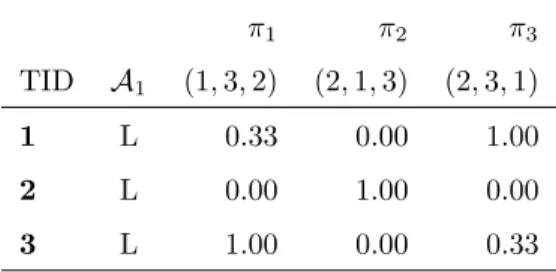
Table 1 shows an example of a Label Ranking dataset represented according to this approach. Instance {A1 =L, π3} (TID=1) contributes to the support

350

Table 1: An example of a Label Ranking dataset. (TID = Transaction ID)

π1 π2 π3

TID A1 (1,3,2) (2,1,3) (2,3,1)

1 L 0.33 0.00 1.00

2 L 0.00 1.00 0.00

3 L 1.00 0.00 0.33

instance, will also give a contribution of 0.33 to the support count of the rule A1=L→π1, given the similarity between their rankings . On the other hand,

no contribution to the support of the ruleA1=L→π2 is given, because these rankings are clearly different. This means thatsuplr(A1=L→π3) =1+0₃.33.

355

Confidence. The confidence of a ruleA→πcomes in a natural way if we replace the classical measure of support with the similarity-basedsuplr.

conf_lr(A→π) = suplr(A→π)

sup(A)

Improvement. Improvement in association rule mining is defined as the smallest difference between the confidence of a rule and the confidence of all sub-rules sharing the same consequent (Section 2.3). In Label Ranking, it is not suitable to

360

compare targets simply as equal or different, as explained earlier. Therefore, to implement pruning based on improvement for Label Ranking, some adaptation is required as well. Given that the relation between target values is different from the classification setting, as discussed earlier, we have to limit the comparison between rules with different consequents, ifs0(π, π0)≥θ.

365

Improvement for LRARs is defined as:

imp_lr(A→π) =min(conf_lr(A→π)−conf_lr(A0→π0))

for∀A0⊂A, and ∀(π, π0) wheres0(π0, π)≥θ.

As an illustrative example, consider the two rulesr1 :A1→(1,2,3,4) and

r2:A2→(1,2,4,3), whereA2is a superset ofA1,A1⊂A2. Ifs0((1,2,3,4),(1,2,4,3))≥

θthenr2 will only be kept if, and only if,conf(r1)−conf(r2)≥minImp.

Lift. This is a measure of the independence between the consequent and the antecedent of the rule [48]. The adaptation oflift for LRAR is straightforward since it only depends the concept of support, for which a version for LRAR already exists:

lift_lr(A→π) = suplr(A→π)

sup(A)·suplr(π)

4.2. Generation of LRAR 375

Given the adaptations of the interestingness measures proposed, the task of learning LRAR can be defined essentially in the same way as the task of learning AR, i.e. to identify a set of LRAR which have a support and a confidence higher than the thresholds defined by the user. More formally, given a training set

D={hxi, πii}, i= 1, . . . , n, the algorithm aims to create a set of high accuracy

380

rulesRπ ={rπ : A → π} to cover a test set T ={hxji}, j = 1, . . . , s. IfRπ

does not cover somexj∈T, adefault ranking (Section 4.3.1) is assigned to it.

4.2.1. Implementation of LRAR in CAREN

The association rule generator2_{we use is CAREN [49]. CAREN implements} an association rule algorithm to derive rule-based prediction models, like CAR

385

and LRAR. For Label Ranking datasets, CAREN derives association rules where the consequent is a complete ranking.

CAREN is specialized in generating association rules for predictive mod-els and employs a bitwise depth-first frequent pattern mining algorithm. Rule pruning is performed using a Fisher exact test [49]. Like CMAR [50], CAREN

390

is a rule-based algorithm rather than itemset-based. This means that, frequent itemsets are derived at the same time as rules are generated, whereas itemset-based algorithms carry out the two tasks in two separated steps.

Rule-based approaches allow for different pruning methods. For example, let us consider the ruleA→λ, whereλis the most frequent class in the examples

395

covering A. If sup(A→λ) < minsup then there is no need to search for a

2

superset ofA, A∗, since any rule of the form A∗ →λ, A⊂ A∗ cannot have a support higher thanminsup.

CAREN generates significant rules [23]. Statistical significance of a rule is evaluated using a Fisher Exact Test by comparing its support to the support

400

of its direct generalizations. The direct generalizations of a rule A → C are

∅→Cand (A\ {a})→C whereais a single item.

The final set of rules obtained define the Label Ranking prediction model, which we can also refer to as thelabel ranker.

CAREN also employs prediction for strict rankings usingconsensus ranking 405

(Section 4.3), best rule, among others.

4.3. Prediction

A very straightforward method to generate predictions using a label ranker is used. The set of rulesRπ can be represented as an ordered list of rules, by

some user-defined measure of relevance:

410

< rπ1, rπ2, . . . , rπs >

As mentioned before, a rule r∗π : A∗ → π∗ covers (or matches) an instance

xi∈T, ifA∗⊆desc(xi). If only one rule,r∗π, matchesxi, the predicted ranking

forxi is π∗. However, in practice, it is quite common to have more than one

rule covering the same instancexi,R∗π(xj)⊆ Rπ. InR∗π(xj) there can be rules

with conflicting ranking recommendations. There simple approaches to address

415

those conflicts, such as selecting the best rule, calculating the majority ranking, etc.

However, it has been shown that a ranking obtained by ordering the average ranks of the labels across all rankings minimizes the Spearman footrule distance to all those rankings [51]. In other words, it maximizes the similarity according

420

to Spearman’sρ[44], and, consequently [52] Kendall’sτ. This can be referred to as theaverage ranking [11].

average ranks as:

π(j) =

s

P

i=1

πi(j)

s , j= 1, . . . , k (2)

The average ranking π can be obtained if we rank the values of π(j), j =

425

1, . . . , k. A weighted version of this method can be obtained by using the con-fidence orsupport of the rules inR∗

π(xj) as weights.

4.3.1. Default rules

As in classification, in some cases, the label ranker might not find any rule that covers a given instancexj, soR∗π(xj) =∅. To avoid this, we need to define 430

adefault rule,r_∅, which can be used in such cases:

{∅} →default ranking

Adefault class is also often used in classification tasks [53], which is usually the majority class of the training set D. In a similar way, we could define the majority ranking as our default ranking. However, some Label Ranking datasets have as many rankings as instances, making the majority ranking not

435

so representative.

As mentioned before, theaverage ranking (Equation 2) of a set of rankings, minimizes the distance to all rankings in that set [51]. Hence we can use the

average rankingof the target rankings in the training data as thedefault ranking.

4.4. Parameter tuning 440

Due to the intrinsic nature of each different dataset, or even of the pre-processing methods used to prepare the data (e.g., the discretization method), theminsup/minconf needed to obtain a rule setRπ, that covers all the

exam-ples, may vary significantly [54]. The trivial solution would be, for example, to setminconf = 0 which would generate many rules, hence increasing the

cover-445

Let us defineM as the coverage of the model i.e. the coverage of the set of rulesRπ. Algorithm 1 represents a simple, heuristic method to determine the

450

minconf that obtains the rule set such that a certain minimal coverage,minM, is guaranteed.

Algorithm 1Confidence tuning algorithm

Givenminsup andstep minconf = 100%

whileM < minM do

minconf =minconf −step

Run CAREN with (minsup,minconf) and determineM

end while

return minconf

This procedure has the important advantage that it does not take into ac-count the accuracy of the rule sets generated, thus reducing the risk of overfit-ting.

455

5. Pairwise Association Rules

Association rules use a sets of descriptors to represent meaningful subsets of the data [55], hence providing an easy interpretation of the patterns mined. Due to the intuitive representation, since its first application for market bas-ket analysis [56], they have become very popular in data mining and machine

460

learning tasks (Mining rankings [5], classification [6], Label Ranking [7], etc). LRAR proved to be an effective predictive model [7], however they are de-signed to find complete rankings. Despite its similarity measures, which take into account ranking noise, they do not capture subranking patterns because they will always try to infer complete rankings. On the other hand, association

465

rules were used to find patterns within rankings [5], but without relating them to the values of the independent variables.

of pairwise comparisons), the Pairwise Association Rules (PAR), which can be

470

regarded as predictive or descriptive model. We define a PAR as:

A→ {λaλb⊕λbλa⊕λa=λb⊕λa ⊥λb | λa, λb∈ L}

where, as in the original AR paper [4], we allow rules with multiple items, not only in the antecedent but also in the consequent. In other words, PAR can also have multiple sets of pairwise comparisons in the consequent.

Similar to RPC (Section 3.1.3), we decompose the target rankings into

pair-475

wise comparisons. Therefore, PAR can be obtained from data with strict, partial and incomplete rankings3_.

Contrary to LRAR, we use the same interestingness measures that are also used in typical AR approaches, instead of the similarity-based versions defined for Label Ranking problems, i.e. sup, conf, etc. This allows PAR to filter out

480

non-frequent/interesting patterns without the need to derive strict rankings. When methods cannot find interesting rules with enough pairwise comparisons to define a strict ranking, then it can abstain from making some choices an, thus, obtain partial rankings, subrankings or even with sets of disjoint pairwise comparisons.

485

Abstention is used in machine learning to describe the option to not make a prediction when the confidence in the output of a model is insufficient. The simplest case is classification, where the model can abstain itself to make a de-cision [57]. In the Label Ranking task, a method that makes partial abstentions was proposed in [30]. A similar reasoning is used here both for predictive and

490

descriptive models. Partial abstentions also make sense in PAR. Hence, the de-cision to abstain on certain pairwise preferences is defined by interest measures, such asminconf orlift.

More formally, let us defineD ={hxi, πii}, i= 1, . . . , n where πi can be a

complete ranking,partial ranking or asub-ranking. For eachπof sizek, we can

495

3_{To derive the PAR, we added a pairwise decomposition method to the CAREN [49]}

extract up tohpairwise comparisons. We consider 4 possible outcomes for each pairwise comparison:

• λaλb

• λbλa

• λa=λb (indifference)

500

• λa⊥λb (incomparability)

As an example, a PAR can be of the form:

A→λ1λ4∧λ3λ1∧λ1⊥λ2

The consequent can be simplified into λ3 λ1 λ4 or represented as a sub-rankingπ= (2,0,1,3).

6. Experimental Results 505

In this section, we start by describing the datasets used in the experiments, then we introduce the experimental setup and finally present the results ob-tained.

6.1. Datasets

The Label Ranking datasets in this work (Table 2) were taken from the Data

510

Repository of Paderborn University4.

To illustrate domain-specific interpretations of the results, we experiment with two additional datasets. We use Algae [58], an adapted dataset from the 1999 COIL Competition [59], concerning the frequencies of algae populations in different environments5_{. The original dataset consisted of 340 examples, each}

515

representing measurements of a sample of water from different European rivers

4_{https://www-old.cs.uni-paderborn.de/fachgebiete/intelligente-systeme/}

software/label-ranking-datasets.html(accessed 10.02.17)

5

on different periods. The measurements include concentrations of chemical sub-stances like nitrogen (in the form of nitrates, nitrites and ammonia), oxygen and chlorine. Also the pH, season, river size and its flow velocity were registered. For each sample, the frequencies of 7 types of algae were also measured. In this

520

work, we considered the algae concentrations as preference relations by ordering them from larger to smaller concentrations. Those with 0 frequency are placed in last position and equal frequencies are represented with ties. Missing values in the independent variables were set to 0.

Finally, the Sushi preference dataset [12], which is composed of demographic

525

data about 5000 people and sushi preferences, is also used. Each person sorted a set of 10 different sushi types by preference. The 10 types of sushi, are a) shrimp, b) sea eel, c) tuna, d) squid, e) sea urchin, f) salmon roe, g) egg h) fatty tuna, i) tuna roll and j) cucumber roll. Since the attribute names were not transformed in this dataset, it is particularly useful for the interpretation

530

of the patterns extracted.

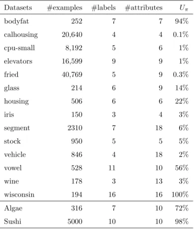
Table 2 also presents a simple measure of the diversity of the target rankings, the Unique Ranking Proportion, Uπ. Uπ is the proportion of distinct target

rankings for a given dataset. As a practical example, the iris dataset has 5 distinct rankings for 150 instances, which results inUπ =₁₅₀5 ≈3%.

535

6.2. Experimental setup

Continuous variables were discretized with two distinct methods: (1)EDiRa

[37] and (2)equal width bins. EDiRais the state of the art supervised discretiza-tion method in Label Ranking, while equal width is a simple, general method that serves as baseline.

540

The evaluation measure used in all experiments is Kendall’sτ(Section 3.2). A ten-fold cross-validation was used to estimate the value for each experiment. The generation of LRAR and PAR was performed with CAREN [49] which uses a depth-first approach.

The confidence tuning method described earlier (Algorithm 1) was used to

545

Table 2: Summary of the datasets.

Datasets #examples #labels #attributes Uπ

bodyfat 252 7 7 94%

calhousing 20,640 4 4 0.1%

cpu-small 8,192 5 6 1%

elevators 16,599 9 9 1%

fried 40,769 5 9 0.3%

glass 214 6 9 14%

housing 506 6 6 22%

iris 150 3 4 3%

segment 2310 7 18 6%

stock 950 5 5 5%

vehicle 846 4 18 2%

vowel 528 11 10 56%

wine 178 3 13 3%

wisconsin 194 16 16 100%

Algae 316 7 10 72%

Sushi 5000 10 10 98%

minconf value can be found in, at most, 20 iterations. Given that a common value for the minsup in association rule mining is 1%, we use it as default, except is stated otherwise. We define the minM as 95%, to get a reasonable coverage, andminImp= 1%, to avoid rule explosion.

550

In terms of similarity functions, we use a normalized Kendallτ between the interval [0,1] as our similarity functions0 (Equation 1).

6.3. Results with LRAR

In the experiments described in this section, we analyze the performance of LRAR from different perspectives, namely accuracy, number of rules and

555

the impact of using similarity measures in the generation of LRAR and provide some insights about its usage.

LRAR, despite being based on similarity measures, are consistent with the classical concepts underlying association rules. A special case is when θ = 1,

560

where, as in CAR, only equal rankings are considered. Therefore, by varying the thresholdθwe also understand how similarity-based interest measures (0≤θ <

1) contribute to the accuracy of the model, in comparison to frequency-based approaches (θ= 1).

We would also like to understand how some properties of the data relate the

565

sensitivity toθ. We can extract two simple measures of ranking diversity from the datasets, the Unique Ranking Proportion (Uπ), described earlier, and the

ranking entropy [37].

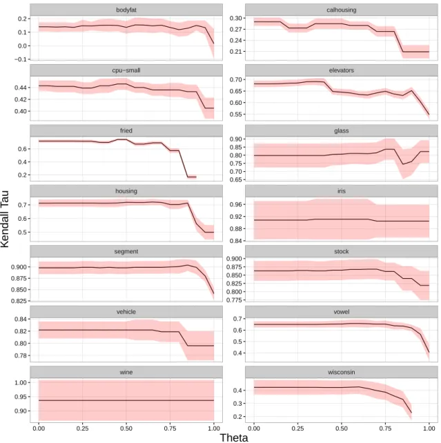
6.3.1. Sensitivity analysis: Accuracy

In Figure 1, we can see the behavior of the accuracy of CAREN varying

570

the value ofθ. It shows that, in general, there is a tendency for the accuracy to decrease as θ gets closer to 1. This happens in 12 out of the 14 datasets analyzed. On the other hand, in 9 out of 14 datasets, the accuracy is rather stable in the rangeθ∈[0,0.6].

If we take into consideration that the model ignores the similarity between

575

rankings forθ= 1, the results indicate that, as expected, there is advantage in using the more flexible approach (i.e. taking ranking similarity into account) compared to the strict classification approach (i.e. using CAR). Two extreme cases arefried and wisconsin, where CAREN was not able to find any LRAR forθ= 16_.

580

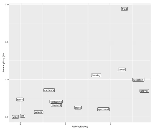
Let us consider theaccuracy range, the maximum accuracy minus the mini-mum accuracy. To find out which datasets are more likely to be affected by the choice ofθ, we can compare their ranking entropy with the measuredaccuracy range (In interest of space, we do not include the specific values here but they

bodyfat calhousing cpu−small elevators fried glass housing iris segment stock vehicle vowel wine wisconsin −0.1 0.0 0.1 0.2 0.21 0.24 0.27 0.30 0.40 0.42 0.44 0.55 0.60 0.65 0.70 0.2 0.4 0.6 0.65 0.70 0.75 0.80 0.85 0.90 0.5 0.6 0.7 0.84 0.88 0.92 0.96 0.825 0.850 0.875 0.900 0.775 0.800 0.825 0.850 0.875 0.900 0.78 0.80 0.82 0.84 0.4 0.5 0.6 0.7 0.90 0.95 1.00 0.2 0.3 0.4

0.00 0.25 0.50 0.75 1.00 0.00 0.25 0.50 0.75 1.00

Theta

K

endall T

au

can be easily estimated from Figure 1). In Figure 2, we compare the accuracy

585

range with theranking entropy [37]. We can see that, the higher the entropy, the more the accuracy can be affected by the choice ofθ.

Results seem to indicate that, when mining LRAR in datasets with low ranking entropy, the choice ofθ is not so relevant. On the other hand, as the entropy gets higher, reasonable values are in the range 0≤θ≤0.6.

590

Another interesting observation can be made regarding fried. Despite the fact that it has a very low proportion of unique rankings, Uπ(fried) = 0.3%

(Table 2) its entropy is quite high (Figure 2). For this reason, it makes it more sensitive toθ, as seen in Figure 1. On the other hand,iris andwine, with very low entropy, seem unaffected byθ.

595

●

●

● ●

●

●

●

●

●

●

●

●

●

●

bodyfat

calhousing

cpu−small elevators

fried

glass

housing

iris

segment

stock vehicle

vowel

wine

wisconsin

0.0 0.2 0.4 0.6

1 2 3

RankingEntropy

Accur

acyDrop (%)

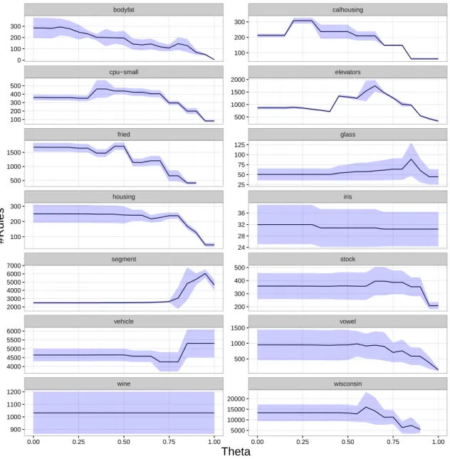
6.3.2. Sensitivity analysis: Number of rules

Ideally, we would like to obtain a small number of rules with high accuracy. However, such a balance is not expected to happen frequently. Ultimately, as accuracy is the most important evaluation criterion, if a reduction in the number of rules comes with a high cost in accuracy, it is better to have more

600

rules. Thus, it is important to understand how the number of LRAR varies with the similarity thresholdθ, while taking the impact in the accuracy of the model into account as well.

In Figure 3, we see how many LRAR are generated per dataset asθ varies. The majority of the plots, 10 out of 14, show a decrease in the number of rules

605

asθgets closer to 1. As discussed before, the accuracy in general also decreases asθ≥0.6, so let us focus onθ∈[0,0.6].

In the intervalθ∈[0,0.6], the number of rules generated is quite stable in 9 out of 14 datasets. In the first half of this interval,θ∈[0,0.3], it is even more remarkable for 13 datasets.

610

We expect the number of rules to decrease as θ increases, however, results show that the number of rules does not decrease so much, especially for values up to 0.3. This is due to the fact thatθis also used in the pruning step (Section 4.1), reducing the number of rules against which the improvement of an extension is measured and, thus, increasing the probability of an extension not being kept

615

in the model. This means that pruning is being effective in the reduction of LRAR. As mentioned before, imp_lr(A→π) not only compares rules A0 → π

whereA0⊂A, but also rulesA→π0 whereS0(π0, π)≥θ. In other words, with theminImplr we are pruning LRAR with similar rankings too.

These results do not lead to any strong conclusions about the ideal value for

620

θ regarding the number of rules. However, they are in line with the previous analysis ofaccuracy.

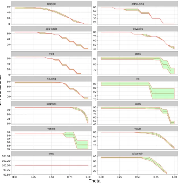
6.3.3. Sensitivity analysis: Minimum Confidence

As described earlier, we use a greedy algorithm to automatically adjust the minimum confidence in order to reduce the number of examples that are not

bodyfat calhousing cpu−small elevators fried glass housing iris segment stock vehicle vowel wine wisconsin 0 100 200 300 100 200 300 100 200 300 400 500 500 1000 1500 2000 500 1000 1500 25 50 75 100 125 100 200 300 24 28 32 36 2000 3000 4000 5000 6000 7000 200 300 400 500 4000 4500 5000 5500 6000 500 1000 1500 900 1000 1100 1200 5000 10000 15000 20000

0.00 0.25 0.50 0.75 1.00 0.00 0.25 0.50 0.75 1.00

Theta

#Rules

covered by any rule. This means that different values of minconf depend on both the dataset and the value ofθ, as seen in Figure 4.

In general, the minconf decreases in a monotonic way as θ increases. As

θ ≈ 1 the minconf gets to its minimum on 13 out of 14 datasets, which is consistent with the accuracy plots (Figure 1). This means that, if we want to

630

generate rules with as much confidence, as measured by minconf, as possible, we should use the minimumθ, i.e.θ= 0.

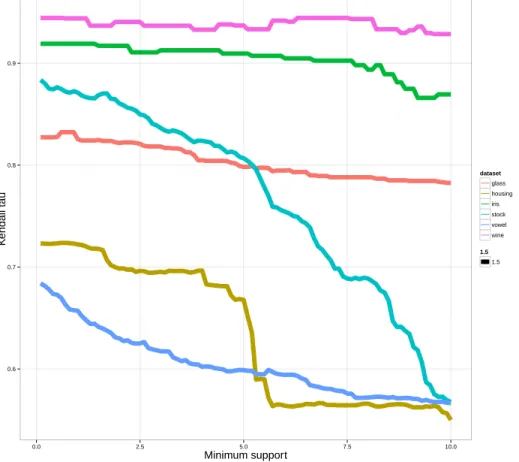
6.3.4. Sensitivity analysis: Support versus accuracy

We vary the minimum support threshold,minsup, to test how it affects the accuracy of our learner. A similar study has been carried out on CBA [60].

635

Specifically, we vary theminsup from 0.1% to 10%, using a step size of 0.1%. Due to the complexity of these experiments, we only considered the six smallest datasets.

In general, as we increaseminsup the accuracy decreases, which is a strong indicator that the support should be small (Figure 5). All lines are

mono-640

tonically decreasing, i.e. either the values remain constant or they decrease as

minsup increases.

From a different perspective, the changes are generally very small forminsup∈ [0.1%,1.0%]. Considering that lowerminsupgenerate potentially more rules, we recommendminsup= 1% as a reasonable value to start experiments with.

645

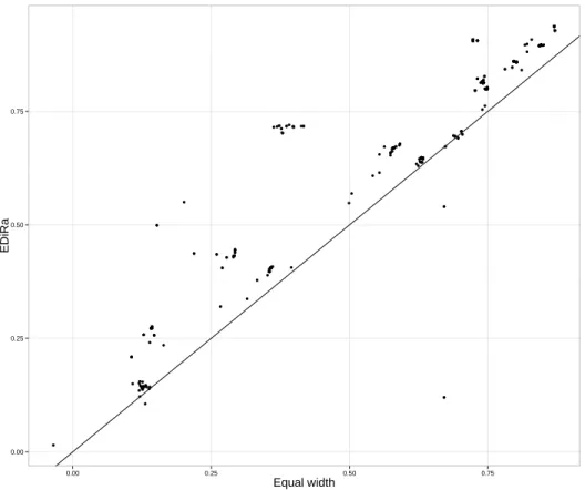
Discretization techniques. To test the influence of the discretization method used, we comparedEDiRa with a non-supervised discretization method, equal width.

In general, the accuracy had the same behavior, as a function of θ, as with

EDiRa, i.e. the results are highly correlated (Figure 6). However, the supervised

650

approach is consistently better. These results add further evidence thatEDiRa

is a suitable discretization method for Label Ranking [37].

bodyfat calhousing cpu−small elevators fried glass housing iris segment stock vehicle vowel wine wisconsin 0 20 40 60 20 30 40 50 60 20 40 60 40 50 60 70 80 0 20 40 60 70 80 90 20 40 60 80 70 75 80 85 90 60 70 80 90 40 50 60 70 80 90 86 88 90 92 94 96 20 40 60 80 99.50 99.75 100.00 100.25 100.50 20 40 60 80

0.00 0.25 0.50 0.75 1.00 0.00 0.25 0.50 0.75 1.00

Theta

Min Confidence

0.6 0.7 0.8 0.9

0.0 2.5 5.0 7.5 10.0

Minimum support

K

endall tau

dataset glass

housing iris

stock vowel wine

1.5 1.5

●● ● ●●● ●●●●●● ● ●● ● ● ● ● ● ● ● ● ● ● ● ● ● ● ● ● ●●●● ● ● ● ● ● ● ● ● ● ● ● ● ● ● ● ● ● ● ● ● ● ● ● ● ● ● ● ● ● ● ● ● ● ● ● ●● ● ● ●●●●● ● ● ● ● ● ● ● ● ● ●●●●● ● ● ● ● ● ● ● ● ● ● ● ● ●●●●●●● ● ●●●●● ● ● ●● ● ● ● ● ● ● ● ● ● ● ● ● ● ●● ● ● ● ● ● ● ● ● ● ● ● ● ● ● ● ●●●●●●● ● ● ● ● ● ● ● ● ● ●●● ● ●● ● ●●●●●●●● ● ● ● ● ● ● ● ● ●●●●●●●●●●● ● ● ● ● ● ● ● ● ● ●●●●●●●●●●●●●● ● ● ● ● ● ● ● ● ● ●●●●●●●●●●● ● ● ● ● ● ● ● ● ● ● ● ● ● ● ● ● ● ● ● ● ● ● ● ● ● ● ● ● ● ●●● ●●●●●●●● ● ● ● ● ● 0.00 0.25 0.50 0.75

0.00 0.25 0.50 0.75

Equal width

EDiRa

Figure 6: Ranking accuracy (Kendallτ) of CAREN after the discretization of data usingequal widthandEDiRa. This plot aggregates all the experiments carried out for each dataset, which

Summary. It is well known that general, simple rules to set parameters of

ma-655

chine learning algorithms do not exist. Nevertheless it is good to know where reasonable values lie. Hence, we think that θ ∈ [0.5,0.6] and minsup = 1% are good default values for LRAR with CAREN. In terms of the discretization methods, our results confirm that a supervised approach, such asEDiRa, is a good choice.

660

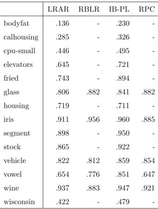
In Table 3 we compare the performance of LRAR with three state of the art approaches, RBLR, which is an alternative rule-based approach [8], IB-PL, an instance-based approach for Label Ranking [31] and Ranking by Pairwise Comparison [24]. We used the parameter values recommended earlier: the data was discretized with theEDiRa method,θwas set to 0.5 andminsupto 1%. It

665

is important to note that the results presented for the other methods are the published results, we did not implement the mentioned approaches.

From Table 3, we see that LRAR are clearly a competitive approach, since their accuracy is in line with the reported values of other approaches. We can conclude that LRAR are able to learn relevant patterns from Label Ranking

670

data.

The lack of results for the RBLR and RPC on some datasets might be due to the size of the rankings in the training data. Both have a decomposition process that transforms the number of training examples inton(k(k−1)/2) examples, wherenis the number of examples in the original data set andkthe number of

675

labels. Because of that the training time can increase dramatically [8].

6.4. Results with PAR

In this work, we use PAR as a descriptive model, to find patterns concerning subsets of labels. We focus in a descriptive task for two reasons. One is to make the approach simpler and the other is to complement the predictive LRAR

680

approach.

Table 3: Results obtained on Label Ranking datasets using 4 different approaches (the mean

accuracy is represented in terms of Kendall’s tau,τ).

LRAR RBLR IB-PL RPC

bodyfat .136 - .230

-calhousing .285 - .326

-cpu-small .446 - .495

-elevators .645 - .721

-fried .743 - .894

-glass .806 .882 .841 .882

housing .719 - .711

-iris .911 .956 .960 .885

segment .898 - .950

-stock .865 - .922

-vehicle .822 .812 .859 .854

vowel .654 .776 .851 .647

wine .937 .883 .947 .921

-Additionally, we set the minimum lift to 1.5. Despite that many interesting

685

rules were found, due to space limitations we only present the most relevant.

Algae data. Using the Algae dataset, we found 179 PARs withminsup= 2 and

minconf = 90. Withsup = 2.2% andconf = 100%, the rule with the highest

lift (approx. 6) was:

Riversize=small∧pH≥37.9∧Flowvelocity=high∧

Chloride≥3.4∧Nitrates&Ammonia≥18.5

→L6L2∧L5L7∧L2L7

The consequent of this rule can be represented asL6 L2 L7∧L5 L7. Considering that the labels represent algae populations, this rule states that it is always true that, under these conditions, type 6 is more prevalent than type 2. It also states that type 7 is less prevalent than types 2, 5 and 6.

690

The rule with the second highestliftobtained, withsup= 3.1% andconf = 91%, is:

Flowvelocity=medium∧Nitrates&Ammonia<18.5∧

Nitrogenasnitrates<7.9

→L1L7∧L7L3

The target of this rule is the partial ranking L1L7 L3. If this PAR was used for prediction, the subrankingπ= (1,0,3,0,0,0,2) would have been the prediction.

Sushi data. When analyzing the sushi dataset we got 166 rules withminconf = 70% andminsup= 1%. The following rule was found, with alift of 1.95:

Ageinterval= 15−19∧Sex=Male∧Livedin=Eastern Japan

→eggseaurchin∧shrimpseaurchin

In the whole dataset, 37% of the people show this relative preferencesegg

seaurchin∧shrimpseaurchin. This PAR shows that this number almost

695

A related rule was also found concerning a different set of people, from a different age group and region (sup= 1.1%,conf = 71.6% andlift= 1.65):

Ageinterval= 30−39∧Sex=Male∧

Livesin=Western Japan∧Changedcity=Yes

→seaurchinegg∧

fattytunatunaroll∧

tunarollcucumberroll∧

fattytunaegg

This rule includes one relative preference found in this group,seaurchinegg, which is the opposite to what was observed in the previous rule. Based on this information, we analyzed the data and found out that 75% of people that live in Eastern Japan preferegg to seaurchinwhile 84% of people from Western

700

Japan preferseaurchinto egg.

7. Conclusions

In this paper, we address the problem of finding association patterns in Label Rankings. We present an extensive empirical analysis on the behavior of a Label Ranking method, the CAREN implementation of Label Ranking Association

705

Rules. The performance was analyzed from different perspectives, accuracy,

number of rules and average confidence. The results show that, similarity-based interest measures contribute positively to the accuracy of the model, in comparison to frequency-based approaches, i.e. whenθ= 1.

The results confirm that LRAR are a viable Label Ranking tool which helps

710

solving complex Label Ranking problems (i.e. problems with high ranking en-tropy). In comparison to other approaches, such as RPC, RBLR and IB-PL, LRAR have the advantage to deliver interpretable results (in the form of asso-ciation rules) and at the same time, without the need to decompose rankings, which saves computational time. The results also enabled the identification of

some values for the parameters of the algorithm that can be used as default values.

Results also seem to indicate that, the higher the entropy, the more the accuracy can be affected by the choice ofθ. The ranking entropy of a dataset can be measured beforehand and the value ofθadjusted accordingly.

720

Additionally, we propose Pairwise Association Rules (PAR), which are as-sociation rules where the consequent represents multiple pairwise preferences. With PAR it is possible to obtain rules with complete, partial and incomplete rankings on the consequent. We illustrated the usefulness of this approach to identify interesting patterns in Label Ranking datasets, which cannot be

ob-725

tained with LRAR.

As future work, we will use PAR for predictive tasks.

Acknowledgments

This work is financed by the ERDF — European Regional Development Fund through the Operational Programme for Competitiveness and

Interna-730

tionalization — COMPETE 2020 Programme within project POCI-01-0145-FEDER-006961, and by National Funds through the FCT — Funda¸c˜ao para a Ciˆencia e a Tecnologia (Portuguese Foundation for Science and Technology) as part of project UID/EEA/50014/2013.

[1] J. F¨urnkranz, E. H¨ullermeier, Pairwise preference learning and ranking, in:

735

Machine Learning: ECML 2003, 14th European Conference on Machine Learning, Cavtat-Dubrovnik, Croatia, September 22-26, 2003, Proceedings, 2003, pp. 145–156. doi:10.1007/978-3-540-39857-8_15.

[2] W. Cheng, J. C. Huhn, E. H¨ullermeier, Decision tree and instance-based learning for label ranking, in: Proceedings of the 26th Annual International

740

[3] S. Vembu, T. G¨artner, Label ranking algorithms: A survey, in: Preference Learning., Springer, 2010, pp. 45–64. doi:10.1007/978-3-642-14125-6_

3.

745

[4] R. Agrawal, R. Srikant, Fast algorithms for mining association rules in large databases, in: VLDB’94, Proceedings of 20th International Conference on Very Large Data Bases, September 12-15, 1994, Santiago de Chile, Chile, 1994, pp. 487–499.

[5] S. Henzgen, E. H¨ullermeier, Mining rank data, in: Discovery Science - 17th

750

International Conference, DS 2014, Bled, Slovenia, October 8-10, 2014. Proceedings, 2014, pp. 123–134. doi:10.1007/978-3-319-11812-3_11.

[6] B. Liu, W. Hsu, Y. Ma, Integrating classification and association rule min-ing, Knowledge Discovery and Data Mining (1998) 80–86.

[7] C. R. de S´a, C. Soares, A. M. Jorge, P. J. Azevedo, J. P. da Costa, Mining

755

association rules for label ranking, in: Advances in Knowledge Discovery and Data Mining - 15th Pacific-Asia Conference, PAKDD 2011, Shenzhen, China, May 24-27, 2011, Proceedings, Part II, 2011, pp. 432–443. doi:

10.1007/978-3-642-20847-8_36.

[8] M. Gurrieri, X. Siebert, P. Fortemps, S. Greco, R. Slowinski, Label ranking:

760

A new rule-based label ranking method, in: Advances on Computational Intelligence - 14th International Conference on Information Processing and Management of Uncertainty in Knowledge-Based Systems, IPMU 2012, Catania, Italy, July 9-13, 2012. Proceedings, Part I, 2012, pp. 613–623.

doi:10.1007/978-3-642-31709-5_62.

765

[9] S. Greco, B. Matarazzo, R. Slowinski, J. Stefanowski, An algorithm for in-duction of decision rules consistent with the dominance principle, in: Rough Sets and Current Trends in Computing, Second International Conference, RSCTC 2000 Banff, Canada, October 16-19, 2000, Revised Papers, 2000, pp. 304–313. doi:10.1007/3-540-45554-X_37.

[10] L. Todorovski, H. Blockeel, S. Dzeroski, Ranking with predictive clustering trees, in: Machine Learning: ECML 2002, 13th European Conference on Machine Learning, Helsinki, Finland, August 19-23, 2002, Proceedings, 2002, pp. 444–455. doi:10.1007/3-540-36755-1_37.

[11] P. Brazdil, C. Soares, J. P. da Costa, Ranking learning algorithms: Using

775

IBL and meta-learning on accuracy and time results, Machine Learning 50 (3) (2003) 251–277. doi:10.1023/A:1021713901879.

[12] T. Kamishima, Nantonac collaborative filtering: recommendation based on order responses, in: Proceedings of the Ninth ACM SIGKDD International Conference on Knowledge Discovery and Data Mining, Washington, DC,

780

USA, August 24 - 27, 2003, 2003, pp. 583–588. doi:10.1145/956750.

956823.

[13] R. Janicki, W. W. Koczkodaj, A weak order approach to group ranking, Comput. Math. Appl. 32 (2) (1996) 51–59. doi:10.1016/0898-1221(96)

00102-2.

785

URLhttp://dx.doi.org/10.1016/0898-1221(96)00102-2

[14] Y. Zhang, D.-Y. Yeung, Multilabel relationship learning, ACM Trans. Knowl. Discov. Data 7 (2) (2013) 7:1–7:30. doi:10.1145/2499907.

2499910.

URLhttp://doi.acm.org/10.1145/2499907.2499910 790

[15] E. Omiecinski, Alternative interest measures for mining associations in databases, IEEE Trans. Knowl. Data Eng. 15 (1) (2003) 57–69. doi:

10.1109/TKDE.2003.1161582.

[16] M. Halkidi, M. Vazirgiannis, Quality assessment approaches in data mining, in: Data Mining and Knowledge Discovery Handbook, 2nd ed., Springer,

795

2010, pp. 613–639. doi:10.1007/978-0-387-09823-4_31.

Conference on Management of Data, San Jose, California, May 22-25, 1995., 1995, pp. 175–186. doi:10.1145/223784.223813.

800

[18] S. Brin, R. Motwani, J. D. Ullman, S. Tsur, Dynamic itemset counting and implication rules for market basket data, in: SIGMOD 1997, Proceedings ACM SIGMOD International Conference on Management of Data, May 13-15, 1997, Tucson, Arizona, USA., 1997, pp. 255–264. doi:10.1145/

253260.253325.

805

[19] J. S. Park, M. Chen, P. S. Yu, Efficient parallel and data mining for association rules, in: CIKM ’95, Proceedings of the 1995 International Conference on Information and Knowledge Management, November 28 -December 2, 1995, Baltimore, Maryland, USA, 1995, pp. 31–36. doi:

10.1145/221270.221320.

810

[20] S. Thomas, S. Sarawagi, Mining generalized association rules and sequential patterns using SQL queries, in: Proceedings of the Fourth International Conference on Knowledge Discovery and Data Mining (KDD-98), New York City, New York, USA, August 27-31, 1998, 1998, pp. 344–348.

[21] J. Han, J. Pei, Y. Yin, R. Mao, Mining frequent patterns without candidate

815

generation: A frequent-pattern tree approach, Data Min. Knowl. Discov. 8 (1) (2004) 53–87. doi:10.1023/B:DAMI.0000005258.31418.83.

[22] R. J. B. Jr., R. Agrawal, D. Gunopulos, Constraint-based rule mining in large, dense databases, Data Min. Knowl. Discov. 4 (2/3) (2000) 217–240.

doi:10.1023/A:1009895914772.

820

[23] G. I. Webb, Discovering significant rules, in: Proceedings of the Twelfth ACM SIGKDD International Conference on Knowledge Discovery and Data Mining, Philadelphia, PA, USA, August 20-23, 2006, 2006, pp. 434–443.

doi:10.1145/1150402.1150451.

[24] E. H¨ullermeier, J. F¨urnkranz, W. Cheng, K. Brinker, Label ranking by

learning pairwise preferences, Artif. Intell. 172 (16-17) (2008) 1897–1916.

doi:10.1016/j.artint.2008.08.002.

[25] V. Chankong, Y. Haimes, Multiobjective Decision Making: Theory and Methodology, Dover Books on Engineering, Dover Publications, 2008. URLhttps://books.google.pt/books?id=o371DAAAQBAJ

830

[26] J. Chomicki, Preference formulas in relational queries, ACM Trans. Database Syst. 28 (4) (2003) 427–466. doi:10.1145/958942.958946. URLhttp://doi.acm.org/10.1145/958942.958946

[27] J. F¨urnkranz, E. H¨ullermeier, Preference learning: An introduction, in: Preference Learning., Springer, 2010, pp. 1–17. doi:10.1007/ 835

978-3-642-14125-6_1.

[28] F. Brandenburg, A. Gleißner, A. Hofmeier, Comparing and aggregating partial orders with kendall tau distances, Discrete Math., Alg. and Appl. 5 (2). doi:10.1142/S1793830913600033.

[29] K. Brinker, E. H¨ullermeier, Label ranking in case-based reasoning, in:

840

Case-Based Reasoning Research and Development, 7th International Con-ference on Case-Based Reasoning, ICCBR 2007, Belfast, Northern Ire-land, UK, August 13-16, 2007, Proceedings, 2007, pp. 77–91. doi:

10.1007/978-3-540-74141-1_6.

URLhttp://dx.doi.org/10.1007/978-3-540-74141-1_6 845

[30] W. Cheng, M. Rademaker, B. D. Baets, E. H¨ullermeier, Predicting par-tial orders: Ranking with abstention, in: Machine Learning and Knowl-edge Discovery in Databases, European Conference, ECML PKDD 2010, Barcelona, Spain, September 20-24, 2010, Proceedings, Part I, 2010, pp. 215–230. doi:10.1007/978-3-642-15880-3_20.

850

Con-ference on Machine Learning (ICML-10), June 21-24, 2010, Haifa, Israel, 2010, pp. 215–222.

[32] S. Har-Peled, D. Roth, D. Zimak, Constraint classification: a new approach

855

to multiclass classification, in: Proc. of the International Workshop on Algorithmic Learning Theory (ALT), Springer-Verlag, 2002, pp. 135–150.

[33] S. Thrun, L. K. Saul, B. Sch¨olkopf (Eds.), Advances in Neural Information Processing Systems 16 [Neural Information Processing Systems, NIPS 2003, December 8-13, 2003, Vancouver and Whistler, British Columbia, Canada],

860

MIT Press, 2004.

[34] G. Lebanon, J. D. Lafferty, Conditional models on the ranking poset, in: Advances in Neural Information Processing Systems 15 [Neural Information Processing Systems, NIPS 2002, December 9-14, 2002, Vancouver, British Columbia, Canada], 2002, pp. 415–422.

865

[35] A. Aiguzhinov, C. Soares, A. P. Serra, A similarity-based adaptation of naive bayes for label ranking: Application to the metalearning problem of algorithm recommendation, in: Discovery Science - 13th International Conference, DS 2010, Canberra, Australia, October 6-8, 2010. Proceedings, 2010, pp. 16–26. doi:10.1007/978-3-642-16184-1_2.

870

[36] C. R. de S´a, C. Soares, A. Knobbe, P. J. Azevedo, A. M. Jorge, Multi-interval discretization of continuous attributes for label ranking, in: Discovery Science - 16th International Conference, DS 2013, Singa-pore, October 6-9, 2013. Proceedings, 2013, pp. 155–169. doi:10.1007/

978-3-642-40897-7_11.

875

[37] C. R. de S´a, C. Soares, A. Knobbe, Entropy-based discretization methods for ranking data, Inf. Sci. 329 (2016) 921–936. doi:10.1016/j.ins.2015.

04.022.

[38] J. Dougherty, R. Kohavi, M. Sahami, Supervised and unsupervised dis-cretization of continuous features, in: Machine Learning, Proceedings of

the Twelfth International Conference on Machine Learning, Tahoe City, California, USA, July 9-12, 1995, 1995, pp. 194–202.

[39] W. Cheng, Label ranking with probabilistic models, Ph.D. thesis, Univer-sity of Marburg (2012).

URLhttp://archiv.ub.uni-marburg.de/diss/z2012/0493 885

[40] J. C. Fodor, M. R. Roubens, Fuzzy preference modelling and multicrite-ria decision support, Vol. 14 of Theory and Decision Library D:, Springer Netherlands, Dordrecht, 1994. doi:10.1007/978-94-017-1648-2.

[41] J. F¨urnkranz, E. H¨ullermeier (Eds.), Preference Learning, Springer, 2010.

doi:10.1007/978-3-642-14125-6.

890

[42] M. Kendall, J. Gibbons, Rank correlation methods, Griffin London, 1970.

[43] A. Agresti, Analysis of ordinal categorical data, Wiley series in probability and mathematical statistics, J. Wiley, Hoboken, 2010.

[44] C. Spearman, The proof and measurement of association between two things, American Journal of Psychology 15 (1904) 72–101.

895

[45] W. H. K. Leo A. Goodman, Measures of association for cross classifications, Journal of the American Statistical Association 49 (268) (1954) 732–764.

[46] J. Pinto da Costa, C. Soares, A weighted rank measure of correlation, Australian and New Zealand Journal of Statistics 47 (4) (2005) 515–529.

doi:10.1111/j.1467-842X.2005.00413.x.

900

[47] J. Pei, J. Han, L. V. S. Lakshmanan, Mining frequent item sets with con-vertible constraints, in: Proceedings of the 17th International Conference on Data Engineering, April 2-6, 2001, Heidelberg, Germany, 2001, pp. 433– 442. doi:10.1109/ICDE.2001.914856.

[48] P. J. Azevedo, A. M. Jorge, Comparing rule measures for predictive

associ-905

on Machine Learning, Warsaw, Poland, September 17-21, 2007, Proceed-ings, 2007, pp. 510–517. doi:10.1007/978-3-540-74958-5_47.

[49] P. J. Azevedo, A. M. Jorge, Ensembles of jittered association rule clas-sifiers, Data Min. Knowl. Discov. 21 (1) (2010) 91–129. doi:10.1007/ 910

s10618-010-0173-y.

[50] W. Li, J. Han, J. Pei, CMAR: accurate and efficient classification based on multiple class-association rules, in: Proceedings of the 2001 IEEE In-ternational Conference on Data Mining, 29 November - 2 December 2001, San Jose, California, USA, 2001, pp. 369–376. doi:10.1109/ICDM.2001. 915

989541.

[51] J. Kemeny, J. Snell, Mathematical Models in the Social Sciences, MIT Press, 1972.

[52] L. Winner, Nascar winston cup race results for 1975-2003, Journal of Statis-tics Education: An international journal on the teaching and learning of

920

statistics 14 (3).

[53] J. Han, M. Kamber, Data Mining: Concepts and Techniques, Morgan Kauf-mann, 2000.

[54] B. Liu, W. Hsu, Y. Ma, Mining association rules with multiple minimum supports, in: Proceedings of the Fifth ACM SIGKDD International

Con-925

ference on Knowledge Discovery and Data Mining, San Diego, CA, USA, August 15-18, 1999, 1999, pp. 337–341. doi:10.1145/312129.312274.

[55] T. Hastie, R. Tibshirani, J. Friedman, The Elements of Statistical Learn-ing: Data Mining, Inference, and Prediction, Springer New York, New York, NY, 2009, Ch. Unsupervised Learning, pp. 485–585. doi:10.1007/ 930

978-0-387-84858-7_14.