Finding ZERO: When No News is Bad News
Hyungshin Park
A dissertation submitted to the faculty of the University of North Carolina at Chapel Hill in partial fulfillment of the requirements for the degree of Doctor of Philosophy in the Kenan-Flagler School of Business.
Chapel Hill 2010
Approved by:
Jeffery Abarbanell
Robert M. Bushman
Raffi J. Indjejikian
Wayne R. Landsman
ii
ABSTRACT
Hyungshin Park: Finding ZERO: When No New is Bad News (Under the direction of Jeffery Abarbanell)
The greater frequency of positive relative to negative earnings surprise in the
distribution of analysts’ forecast-based earnings surprises is well known. If the market
anticipates the propensity of managers to generate positive surprises by biasing earnings
or forecasts, then some of the common assumptions made in the information content
studies are violated. In this paper I provide a rational framework that predicts and
empirical tests that document that zero earnings surprises produce significantly negative
stock price reactions, on average, and increasingly negative a firm’s ex ante probability
of generating a positive earnings surprise. If the greater frequency of positive than
negative earnings surprises in typical earnings surprise distributions is attributable to bias,
then a rational market framework also predicts that the slope coefficient and the
y-intercept in abnormal return-earnings surprise regressions will be negatively correlated; a
result that I also confirm in my empirical tests. These results have important implications
for studies that examine the stock price effect of earnings surprises that meet or fail to
meet hypothesized “bright lines” when empirical tests involve comparing CARs or ERCs
for observations to the left and right of the bright line. Specifically, if such tests do not
take into account the ex ante probability of positive earnings surprise inferences can be
confounded. I review a selection of studies that conclude that there are asymmetric
iii
drawn from announcement abnormal returns and earnings response coefficients can be
iv
v
ACKNOWLEDGEMENTS
I am thankful for the helpful comments and advice from each of my dissertation
committee members: Jeff Abarbanell (Chair), Robert Bushman, Raffi Indjejikian, Wayne
Landsman, and Mark Lang. I am also thankful to John Hand, Ashraf Jaffer, Eva Labro,
Ed Maydew, Chris Petrovits, and all the professors and students at UNC for additional
vi
TABLE OF CONTENTS
LIST OF TABLES ... viii
LIST OF FIGURES ... ix
CHAPTER I. Introduction ...1
II. The model and empirical hypotheses ...7
The propensity for positive earnings surprises ...7
A model of rational responses to biased earnings surprises ...10
Empirical hypotheses ...12
III. Data and preliminary findings ...15
Sample selection ...15
Descriptive statistics and preliminary findings ...17
IV. Empirical results ...20
Hypotheses 1a and 1b ...20
Hypotheses 2 ...23
Robustness tests ...25
Hindsight biases in surprises ...25
Changing the cutoff used to define PPS ...27
V. Interpreting prior literature using a rational framework ...27
vii
Purported penalties to surprises that taken on specific values ...30
The “Meet or Beat” literature ...34
VI. Summary and conclusion ...35
APPENDICES ...57
viii
LIST OF TABLES
Table
1. Descriptive statistics ...38
2. Positive-to-Negative earnings surprise ratios by PPS quintiles ...39
3. Abnormal return around earnings announcement for zero earnings surprise ...41
4. Finding ZERO ...42
5. The relation between the y-intercept and slope in a regression of CAR on earnings surprise ...44
6. Robustness test ...47
7. The relation between the probability of a positive surprise and market-to-book or price-to-earnings ratios ...48
ix
LIST OF FIGURES
Figure
1. The ratio of positive-to-negative earnings surprises over time ...52
2. Firm’s potential reporting choices ...53
3. Graphical summary of Empirical Hypotheses ...54
4. The ratio of positive-to-negative earnings surprises by PPS ...55
1. Introduction
Evaluating the information content of earnings announcements has been a core
issue in financial accounting research dating back to Ball and Brown (1968) and Beaver
(1968). A conceptual underpinning of the information content literature is the notion that
an earnings surprise of exactly zero will generate a neutral (i.e., zero) price response.
While measures of earnings surprises in the literature have evolved and expanded over
time, empirical researchers have typically maintained the implicit assumption that the line
of demarcation between good and bad news (either of which would be expected to
generate a non-neutral stock price response) is a zero surprise, independently of the actual
empirical distributions of earnings surprises.
In this paper I appeal to the results of prior empirical and theoretical studies to
advance a framework that describes how the market would anticipate the possibility that
managers systematically bias earnings surprises; a possibility that has been linked to the
greater frequency of small positive surprises relative to small negative surprises in typical
distributions of analysts’ forecast errors. I present empirical results that are consistent
with the predictions of this framework and contradict the traditional “neutral reaction”
assumption. I also demonstrate the relevance of these findings by showing how
accounting for the propensity of firms to report positive earnings surprises alters
inferences of asymmetric price responses around hypothesized bright lines drawn from
2
surprises on their ex post sign and magnitude (e.g., Skinner and Sloan 2002 and Keung,
Lin and Shih 2009).
Figure 1 presents empirical evidence that motivates my research questions. It
depicts the frequency of positive-to-negative surprises, PTN, for non-zero analyst
forecast-based surprises within an absolute value of 2, 5 and 10 cents, respectively, for
the years 1993 to 2008. Analyst forecast-based earnings surprises, denoted ES, are
measured as IBES reported EPS less IBES consensus analyst EPS estimates. It is evident
in the figure that the frequency of positive surprises is consistently greater than negative
surprises of a similar magnitude over the sample period. The imbalance is greatest for
surprises of smaller absolute magnitudes and varies non-monotonically over time.1
Evidence consistent with that depicted in figure 1 has been reported in the literature
on analyst forecast errors for over a decade (Degeorge, Patel and Zeckhauser 1999,
Matsumoto 2002, Abarbanell and Lehavy 2003b, Dechow, Richardson and Tuna 2003,
Brown and Caylor 2005, and Keung, Lin and Shih 2009). Many related studies that
attempt to explain the propensity for positive earnings surprises identify the role of
strategic earnings management and/or forecast management intended to influence stock
price.2
Based on these explanations and the empirical evidence, I address the following
research questions: do prices respond to earnings surprises in a manner consistent with a
market that anticipates firms’ propensity for generating positive earnings surprises? If so,
1
In this study I focus on the relative frequency of earnings surprise observations that fall in a small interval around and including zero because the overwhelming majority of ex post earnings surprises belong to this region, and also because most studies that hypothesize asymmetric market reactions to surprises that meet or fail to meet certain thresholds focus on surprises in this region.
2There is also a large literature that examines the extent to which scaling surprises by stock price is the
3
what are the implications for empirical tests of asymmetric or discontinuous responses to
“bright line” earnings surprises that are likely to be affected by this propensity?
To answer these questions, I provide a parsimonious model to summarize the
expected impact on the stock price reactions to earnings surprises when market prices
anticipate the propensity of managers to generate biased earnings surprises. This simple
model illuminates essential intuitions gleaned from prior theoretical studies that analyze
the consequence of management misreporting. For example, Fisher and Verrecchia (2000)
(hereafter FV) demonstrate that the presence of positive bias in earnings will produce a
negative average price response in a rational market and this negative market response
increases in the propensity for management to inflate earnings (see FV, corollary 2).3
Furthermore, FV suggest that the magnitude of the average negative response will be
inversely related to the earnings response coefficient (ERC). This occurs because, when
reporting bias is present, for a given change in any exogenous parameter, the intercept in
a regression of returns on earnings surprises adjusts in the opposite direction from the
direction that parameter change moves the ERC.4
One implication of these findings is that negative price response will be observed in
the cross-section for exactly zero surprises when the market expects firms, on average, to
produce positive surprises. If such a propensity is present, then the “neutral reaction”
assumption implicitly adopted in traditional information content papers is violated. In
fact, depending on the propensity to bias surprises upward, it is possible for even small
3
A similar response would be predicted in the earlier model offered in Stein (1989).
4The earnings response coefficient is endogenously determined in FV. Specifically, it is increasing in the
4
realized positive surprises to produce, on average, negative price responses in the
cross-section. Thus, in a rational market, surprises of equal magnitude but of opposite signs
would be expected to generate abnormal returns of different absolute magnitude if there
is an expected difference in their relative frequency.
Another, more subtle, consequence of the preceding equilibrium is that when
surprise realizations are grouped by the ex ante probability that a firm reports a positive
surprise, firms with a higher propensity for positive surprises are expected to have higher
ERCs and more negative intercepts than those with a lower propensity. This prediction
can be used to assess the validity of conclusions in prior literature that hypothesize that
the market either rationally or irrationally rewards (penalizes) earnings surprises that
exceed (falls short of) a hypothesized bright line when such conclusions are based on
comparisons of ERCs or average stock returns of surprises on either side of that bright
line.
I present empirical results that are consistent with a market that anticipates the
propensity for managers to generate positive surprises. Specifically, I find a significantly
negative mean (median) three-day announcement return of -1.07% (-0.75%) to exactly
zero surprises.5 I employ a rolling-window logit model adapted from Barton and Simko
(2002) and apply out-of-sample coefficients to in-sample variable values to calculate the
probability of positive surprise ( PPS) and find that the highest quintile of PPS produces a
significantly negative mean size-adjusted return of -1.87% while the lowest PPS quintile
5Baber, Chen, and Kang (2006) and Keung, Lin, and Shih (2009) also find a mean negative announcement
CAR for zero surprises and attribute it to strategic behavior by managers. However, neither study
5
produces an insignificant mean size-adjusted return of 0.07%.6 Furthermore, I estimate
that the actual level of ES that corresponds to a neutral stock price reaction is between +1
and +2 cents for high PPS quintile firms and close to 0 cents for low quintile firms over
the sample period. Finally, I also find that ERCs and intercepts in regressions of returns
on surprises of small magnitude are negatively associated and also demonstrate how they
move in concert to reflect the functional relation with PPS.
The preceding results have important implications for conclusions concerning the
existence and potential causes of apparent asymmetric rewards or penalties to bright line
earnings surprises drawn in prior studies.7 Specifically, my results suggest that the
combination of accepting the empirical validity of the neutral reaction assumption and/or
sorting earnings surprises on their realized values will almost certainly produce the
appearance of asymmetric responses to bright line surprises in standard tests that compare
abnormal returns or ERCs on either side of hypothesized bright lines. That is, if the
market behaves as if it anticipates incentive-induced biases in surprise measures
employed by researchers, then adherence to standard empirical designs will generate
statistical results that lend credence to hypotheses that are founded on the supposition that
there are asymmetric rewards or penalties to surprises that fall on either side of an
arbitrarily chosen bright line.
I present evidence that variables that have been used to condition earnings surprises
in tests of bright line theories, such as ex ante price-to-earnings (PE) and market-to-book
(MB) ratios, are positively correlated with my measure of PPS. I further show how this
6
The cross-sectional relations I document also hold over time. Specifically, I find a negative serial
correlation between the PPS measure and returns to exactly zero earnings surprises over the sample period.
7I emphasize that this study does not speak directly to the internal validity of hypotheses that predict there
6
empirical fact confounds the interpretation of evidence from prior studies that test
hypotheses that predict asymmetric price responses to bright line surprises but do not
control for the propensity for positive earnings surprises observed in figure 1.
The remainder of the paper proceeds as follows. In section 2, I motivate my
empirical hypotheses with arguments and evidence from the empirical literature on
earnings surprises and theoretical results concerning the expected consequences for
abnormal returns and ERCs of managerial misreporting in a rational market. In section 3,
I describe the sample selection procedures and data used in the empirical tests. Section 4
presents the results of empirical tests of the main hypotheses along with robustness tests.
In section 5, I present evidence of the impact of controlling for the propensity for positive
surprises on inference drawn from prior studies that conclude there are asymmetric or
discontinuous responses to hypothesized bright line surprises. Section 6 contains a
7
2. The model and empirical hypotheses
In this section I parse the extensive literature on earnings surprises and identify
broadly representative studies that refer to strategic incentives for management to
manipulate surprises in order to gain direct or indirect benefits linked to the firm’s stock
price. I do not perform a complete review of these literatures or attempt to challenge the
results or conclusions reached in these studies. Rather, the motivation for this exercise is
to demonstrate that there are ample empirical findings and arguments in the extant
literature to justify the generic strategic equilibrium that includes reporting biases
described below.
2.1. The propensity for positive earnings surprises
Studies that rely on or analyze analyst forecast-based surprises generally assume
that when earnings are exactly equal to the outstanding forecast there is no earnings news
in an announcement. However, there is abundant empirical evidence of peculiarities in
distributions of surprises and related explanations for their cause that raise question about
the validity of this assumption. For example, one stream of literature that investigates the
distributional properties of analyst forecast-based surprises links the greater frequency of
small positive forecast errors than small negative forecast errors in the cross-section to
the possibility of earnings inflation (Degeorge et al. 1999, Bartov, Givoly and Hayn 2002,
Matsumoto 2002, and Burgstahler and Eames 2006). Abarbanell and Lehavy (2003a) find
8
asymmetry” in the distribution of analyst forecast-based surprises that is both predictable
and associated with firms’ stock price sensitivity to earnings news. 8
Another stream of research that examines biases in earnings surprise distributions
identifies managerial actions that influence analysts’ forecasts (Bartov et al. 2002,
Matsumoto 2002, and Richardson, Teoh and Wysocki 2004). These studies focus on the
possibility that analysts are induced (consciously or unconsciously) by managers to bias
their forecasts relative to the earnings managers intend to report. Regardless of the exact
nature of the equilibrium hypothesized, the most recent studies in this literature have
repeatedly pointed to the greater incidence of small positive surprises relative to small
negative surprises as evidence of induced pessimism in analyst forecasts.9
The studies cited above, and others in the earnings management literature, rely on
the argument, or at least entertain the possibility, that firms manage earnings or
manipulate forecasts to secure direct or indirect benefits from a higher stock price. The
direction of causality in the link between managerial incentives to inflate earnings or
induce analyst pessimism to produce positive surprises is sometimes difficult to pin down
in these studies. However, a common thread among them is an appeal to the notion that
8Theories that point to strategic management behavior as the direct or indirect cause of bias in ex post
distributions of earnings surprises also assume there are factors that prevent systematic biases from being eliminated from surprises over time (see Abarbanell and Lehavy 2003b for a discussion of why analysts would not adjust their forecasts to anticipated biased earnings). I do not attempt to explain how such equilibria can arise. Rather, I proceed from the perspective that such factors can be present (as the evidence in figure 1 seems to strongly suggest) in a rational market, and assess whether stock price responses behave in a manner that is consistent with a market that anticipates them on average.
9Earlier studies by Francis and Philbrick (1993) and Lim (2001) posit that analysts bias their forecasts
9
firms that beat hypothesized benchmarks earn equity rewards (Barth, Elliot and Finn
1999, Bartov et al. 2002, Kasznick and McNichols 2002, Lopez and Rees 2002).
Presumably, managers’ decisions to manipulate surprises would be linked to managers’
perceptions of their ability to move stock prices using earnings news (i.e., stock price
sensitivity to earnings news).
Other studies link managers’ incentive to produce positive surprises to efforts to
exploit private information over limited timeframes (Bartov and Mohanram 2004 and
Richardson, Teoh and Wysocki 2004). Bartov and Mohanram, for example, posit that
managers produce positive surprises relative to analysts’ forecasts to maintain high stock
prices during a period in which they exercise stock options and sell shares. Subsequently,
their firms report the disappointing earnings news that had been withheld by managers.
Once again, the incentive to engage in such behavior is presumably tied to managers’
perception of the stock price sensitivity to earnings news. In sum, the general tenor of the
representative selection of studies cited above is that bias is more beneficial to managers
and more likely to occur when stock price is highly sensitive to earnings news. My
formulation below reflects this assumption.10
10
2.2. A model of rational responses to biased earnings surprises
Let i = the true earnings of firm i
i
s = the surprise relative to the market’s prior expectation of earnings of firm i
i i
i
i E s s
r [ ] 0 = the reported earnings of firm i
] | [ i i
i E r
V = the market value of firm i given ri
= positive earnings multiple exogenously given
A firm manager privately observes true earnings,i, where i is drawn from a
uniformly distributed discrete random variable ~
with mean 0 and support (,).
The manager can disclose ri i or ri i s, where s is a positive constant.
11
Figure
2 depicts the possible reporting choices of firms at each level of true earnings. In order to
disclose ri i s, the firm manager must incur a personal cost of
2
s
ci , which could
reflect psychic costs, or the costs of lost reputation or legal liability in the (uncertain)
event that misreporting is subsequently discovered and penalized. The random cost of
unit inflation (ci) is privately known by the manager at the time of the report and is
11While the analysis I present explicitly contemplates surprises that result from the inflation of true earnings
11
drawn from the uniform distributionU[a,b].I impose a regularity condition b s
a to
avoid corner solutions.
When the manager discloses ri investors make an inference about the manager’s
reporting choice. The investor’s valuation of a firm is:
] |
[ )
(ri 0 si E i ri 0 si
V (1)
where the earnings multiple, , is an exogenously given positive number.12
The manager’s utility function is a linear sum of firm value and the personal cost of
earnings management. In particular, his utility function is:
) (ri 0 si
V if si (i 0) (2)
2
0 )
(r s c s
V i i i if si (i 0)s (3)
Suppose investors believe that the manager’s reporting choice depends on the
manager’s observation of ci ci, and that there exists a threshold, ˆ , above which the
manager reports ri i and below which he reports ri i s.
13
Letpˆ prob(ci ˆ) ,
then the equilibrium value of the threshold is:
12A reasonable objection to this formulation is that it does not account for investors’ expectation of bias in
earnings from previous periods. For example, in a multi-period model with some settling up, investors could learn precisely which firms are going to bias surprises and unravel it completely and managers would have no obvious reason for manipulating surprises. It should be clear, however, that the empirical predictions from my model are founded on the assumption that some residual investor uncertainty (or incomplete learning) is present in any given period, which includes the possibility that investors imperfectly observe the manager’s objective function (see FV for a similar construction). Therefore, for the sake of simplicity, I do not explicitly model the impact of previous expected bias in earnings surprises.
12 s
ˆ (4)
Proof: (see appendix 1)
To summarize, managers have private information regarding true earnings and also
the manager-specific cost of biasing surprises upward through earnings and/or forecast
manipulation. Managers must assess the trade-off between the stock price benefit of
managing surprises and the personal cost of doing so. Investors have imperfect
information about this tradeoff for individual firms and use it to establish stock price. As
a result, there exists an equilibrium threshold for the cost of biasing surprises, under
which firms inflate the surprise and above which they do not. A key feature of this
equilibrium is that the investors cannot discern whether a specific firm has actually
biased the surprise by observing it ex post, however, they are aware of the possibility that
individual firms will do so and adjust the price associated with actual surprises for the ex
ante probability that bias is present.
2.3. Empirical hypotheses
In the preceding equilibrium investors form an expectation of the probability the
manager will strategically bias the earnings surprise and discount that surprise by the
amount of the expected bias.
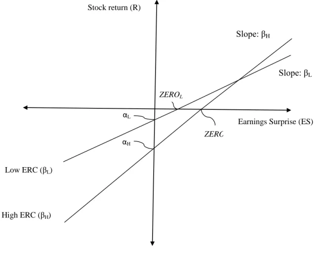
Hypothesis 1a: The average stock return to a zero surprise is negative and increasingly negative in the probability a firm will report a positive surprise
Hypothesis 1a, which follows from the second and the third comparative statics in
13
possibly small positive forecast errors all to be negative, and more negative as the ex ante
probability of positive surprise management increases. This is because, in equilibrium,
rational investors anticipate that firms with a non-zero probability of generating a positive
surprise will manage the surprise to a positive number (even if the firm does not actually
do so because the privately observed cost of biasing surprises is too high), therefore zero
or even small positive forecast errors will constitute a disappointment to the investors. In
addition, investors anticipate firms with a greater ex ante probability of surprise
management will produce an even greater earnings surprise, and, therefore, a zero
surprise for these firms would be an even greater disappointment to the investors. That is,
if the model is descriptively valid it should also be the case that:
Hypothesis 1b: The level of earnings surprise that corresponds to a neutral stock price reaction is a small positive number and increases in the probability that a firm reports a positive surprise
Hypothesis 1b, which follows from the fourth and fifth comparative statics in
appendix 1, implies that the measurement error inherent in assuming that the line of
demarcation between a good news and bad news surprise is zero increases in the
probability that a firm manages its earnings surprise. Alternatively, the level of surprise
that actually corresponds to “no news” becomes more positive as the probability of a
positive surprise increases. Figure 3 presents a graphical summary of the hypotheses.
The following hypothesis is relevant to the interpretation of regression-based tests
of price responses to earnings surprises:
14
Hypothesis 2: In a regression of returns on earnings surprises the earnings response coefficient and the intercept are negatively correlated
Hypothesis 2, which follows from the third comparative static in appendix 1,
predicts a negative correlation between a stock’s earnings response coefficient, β, i.e., the
slope in the regression of returns on surprises, and the average stock return, α, i.e., the
y-intercept in the regression. This follows because investors are aware of the fact that firms
with higher ERCs are more likely to generate a positive earnings surprise due to greater
(more severe) stock price benefit (penalty) to reporting higher (lower) earnings and will
establish a discount for the expected surprise even before the actual earnings are known
to or reported by the manager. The higher is the ERC, the greater is that expected
discount.
The results of the model I present in this section suggest that if empirical tests of
theories that predict strategic biases in surprises do not address the expected propensity
for biased surprises, the conclusion of asymmetric responses to bright line surprises will
likely be a self-fulfilling prophecy when a rational market anticipates bias in distribution
of earnings surprises. In addition, some studies implicitly assume or explicitly
hypothesize an inefficient (correction of a previously inefficient) market response (price
level) to surprises that meet or fail to meet a particular bright line. Either type of
argument leads to an expectation of an asymmetric price response to surprises on either
side of the relevant threshold. While such theories may in fact be descriptive of the world,
the preceding hypotheses have implications for tests of these theories that rely on
comparing abnormal returns or ERCs but do not take into account the propensity for
15
3. Data and preliminary findings
3.1. Sample Selection
My sample includes all available quarterly earnings announcements between 1993
and 2008. I test my main hypotheses using earnings surprises based on analysts’ forecasts.
I choose 1993 as the beginning of my sample period for two reasons. First, this cutoff
ensures the congruence of IBES and COMPUSTAT announcement dates. Dellavigna and
Pollet (2009) report that the IBES announcement date and the COMPUSTAT
announcement date generally agree after 1988, whereas before 1989 there are many cases
where these two dates do not agree. Second, Abarbanell and Lehavy (2007) document a
regime shift in the IBES database around 1991-1992, which affects the distributional
properties of analysts’ forecast-based earnings surprises, and suggest that longitudinal
studies that straddle the year 1991-1992 but do not account for this shift may generate
erroneous inferences.
Analyst forecast-based earnings surprises, ES, are calculated as IBES reported EPS
less the consensus analyst forecast of EPS. For each earnings announcement I collect EPS
and the most recent consensus analyst EPS forecast prior to the announcement from the
stock-split unadjusted IBES dataset.14 I restrict the period between the consensus forecast
and the announcement date to be less than or equal to 31 days in order to eliminate stale
forecasts. The resulting number of ES observations is 237,535.
14I use the median analysts’ forecast as the consensus EPS forecast, but the results are qualitatively similar
16
I use CRSP to calculate three-day buy-and-hold size-adjusted stock returns (-1, 1)
around the announcement in order to assess the market’s reaction to the earnings
surprise.15 Size-adjusted returns are the excess stock returns over the corresponding
size-deciles portfolio returns. Size-size-deciles portfolio returns are calculated by ranking firms
into deciles by the market value of equity at the beginning of the quarter.
A key variable in my study is the probability of a positive surprise, PPS. I construct
this variable from a logit regression adapted from Barton and Simko (2002). In order to
obtain an up-to-date estimate of PPS prior to each announcement, I estimate logit
regressions in twelve-quarter rolling-windows following the methodology in Cheng
(2006) as opposed to the pooled regressions employed in Barton and Simko. In addition,
if any variables that are originally defined in Barton and Simko are not available to the
market at the time of earnings announcement, they are replaced by the most recent values
that were available. For example, I replace the current market-to-book ratio, MB, in
Barton and Simko with the last quarter’s MB. Because of the twelve-quarter rolling
window estimation procedure, the earliest time period that PPS becomes available is the
first quarter of 1996. The estimation procedures and descriptive statistics for the variables
used to construct PPS are presented in appendix 2.
The total number of quarterly earnings announcements with non-missing EPS,
consensus analyst forecasts, and the variables required for the PPS calculation is 95,613.
However, the requirement of three years for the PPS estimation period further reduces the
sample size to 82,992.
15Alternatively, I calculate abnormal returns using three different metrics: market-adjusted, market-model
17 3.2. Descriptive statistics and preliminary findings
Descriptive statistics for the main variables are presented in panel A of table 1. All
variables except for PPS are winsorized at 1% and 99% to reduce the effects of ouliers.
The skewness measure and comparisons of the 95th to the 5th percentiles of ES
distribution indicate a longer negative tail, consistent with prior evidence reported in
Abarbanell and Lehavy (2003b). The mean ES is small but significantly negative in my
sample, while the median is slightly positive and significant. Early studies of analyst
forecast errors typically reported a large negative mean error. However, this finding is
consistent with conclusions of declining apparent mean optimism in errors reported in
more recent studies and evidence of change in IBES procedures as to which items to
include in forecasts and reported earnings after 1991 (Brown and Caylor 2005 and
Abarbanell and Lehavy 2007) The fact that the surprises are not scaled by price, as is
frequently the case in prior studies, also contributes to this finding.
Summary statistics for the PPS measures indicate negative skewness in the
distribution, but confirm a higher expected incidence of positive surprises in the sample.
These results are consistent with the distributional evidence of the relatively greater
frequency of positive than negative surprises in the cross-section and over time in figure
1, and provide support for the possibility that investors have the ability to predict the
propensity for small positive surprises commonly found in empirical distributions of ex
post surprises.
Summary statistics for MB ratios are on par with those reported by Barton and
Simko (2002). In untabulated results I find that the mean and median values of MB and
18
the requirement of analysts’ forecasts. The CAR measure produces descriptive statistics
that are consistent with other estimates of size-adjusted returns in the literature. The
distribution of announcement CARs appears to be nearly symmetric and centered very
close to zero.
The correlation matrix in panel B of table 1 indicates a positive association between
the ES and PPS, consistent with the argument that an ex post surprise is increasing in the
ex ante estimate of the probability of a positive surprise. Another interesting preliminary
finding in panel B is the significant positive association between PPS and both the PE
and MB ratio. This finding continues to hold even when MB is excluded as an
explanatory variable from the estimation of PPS. The result suggests that the level of
these ratios may serve as a coarse proxy for the ex ante probability of a positive surprise,
which, in turn, raises questions about the interpretation of conclusions concerning
asymmetric price responses around surprise thresholds when data is grouped in the levels
of these variables. I elaborate on this finding in section 5.
Panel A of table 2 reports the ratio of positive-to-negative surprises, PTN, for
non-zero surprises of an absolute magnitude of 2, 5 and 10 cents, respectively, by PPS quintile.
PTN increases monotonically from 1.07 to 5.09 in PPS quintile. Figure 4 summarizes the
relation between PPS and PTN by high, middle and low quintile over the sample period,
where the three middle PPS quintiles are assigned to the middle group. PTN is monotonic
in quintile of PPS in every sample year.
Panel B of table 2 (top table) shows the number of observations for each level of
earnings surprise by PPS quintiles. In contrast to some variations of “bright line” theories
19
one cent earnings surprises, the frequency of earnings surprise is clearly increasing in
PPS for all non-negative earnings surprises, i.e., the distribution shifts to the right
conditional on PPS. The bottom table of panel B reports the mean values of PPS for
given earnings surprise levels by PPS quintile. As expected, the mean PPS increases
across PPS quintile for the same earnings surprise but is stable across earnings surprises
levels for the same PPS quintile. I will revisit the results of this table in section 5.2.
Panel C of table 2 reports results related to the time series correlation between PTN
and PPS by quarter. Model 1 presents the results of a regression of quarterly PTN on
quarterly PPS. The coefficient is positive and highly significant. Model 2 includes the
time variable. The results indicate a small, but significantly negative time trend in PTN
for my sample, which is inconsistent with an increasing demand for firms to produce
positive surprises suggested by Matsumoto (2002) and Bradshaw and Sloan (2002), but
consistent with a decreasing trend in the incidence of positive surprises documented in
Koh, Matsumoto and Rajgopal (2008) who argue that firm incentives to produce a
positive surprise have diminished subsequent to celebrated accounting scandals. Most
relevant for my study, however, is that the correlation between PTN and PPS over time
remains positive and highly significant.
The evidence in table 2 and figure 4 demonstrates that PPS is highly correlated with
the PTN both in the cross-section and over time. The results provide assurance that an ex
20
4. Empirical Results
4.1. Hypotheses 1a and 1b
Hypothesis 1a predicts that the average stock returns to a zero forecast error will be
negative and become more negative for firms with a greater probability of surprise
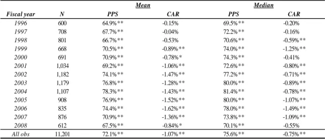
management. Panel A of table 3 reports three-day size-adjusted abnormal returns to zero
earnings surprises for each year of the sample. Mean and median PPS values exceed 50%
in every year and mean and median CARs are negative in every year. Negative mean
(median) CARs are statistically significant in 10 of 13 (9 of 13) years. The results for the
entire sample period, which are consistent with average earnings announcement abnormal
returns results reported in Baber, Chen and Kang (2006), and Keung, Lin and Shih (2009)
are highly significant.
The evidence in panel A of table 3 also suggests a relation between the level of PPS
and the size of the average negative return to a zero surprise. That is, years with higher
average levels of PPS produce larger negative returns to zero earnings surprises than
years with relatively lower values of PPS. For example, the mean values of PPS are
relatively high, ranging from 74.1% to 78.3% in 2002-2006 periods. These years produce
negative CARs that range from -1.28% to -1.62%. In untabulated results I find that the
correlation between PPS and CARs for zero surprises is -0.08 (significant at 1% level). It
is also interesting to note that neither PPS nor CARs for zero surprises are monotonic
over the years, suggesting that overall incentives to bias surprises and market reactions to
such biases vary in the cross-section over time.
Panel B of table 3 presents additional evidence on hypothesis 1a. The first (second)
21
3 sub-periods (1996-1999, 2000-2004, and 2005-2008) and for the entire sample period.
There is a monotonic relation between the level of PPS and CARs. Mean (median) CARs
range between an insignificant 0.07% (-0.25%) for the 1st quintile of PPS to a significant
-1.87% (-1.22%) for the 5th quintile for the entire sample period. A test of differences
between the 5th and 1st quintile is highly significant. Similar results are observed for all
sub-periods.
Hypothesis 1b is the flipside of hypothesis 1a, which is the level of surprise that
generates a neutral price response is positive and increasing in the probability of a
positive surprise. Tests of this hypothesis are intended to provide a numerical feel for the
amount of surprise in EPS necessary to generate a neutral response, and can be thought of
as a method of calibrating earnings surprises in tests of price reactions to earnings news;
i.e., producing an estimate of the earnings surprise that will generate a neutral stock
response, denoted ZERO.
Preliminary evidence related to hypothesis 1b is presented in panel A of table 4,
which reports mean size-adjusted stock returns to small earnings surprises of magnitudes
ranging from -10 cents to +10 cents after partitioning by quintile of PPS. Differences in
returns between the lowest and highest quintile are presented in the last column. The
mean return to the lowest quintile of PPS significantly exceeds that associated with
highest quintile for earnings surprises that range from -5 cents up to +2 cents. Differences
are insignificant for surprises out of this range. This indicates that investors are generally
more disappointed when high PPS firms just miss, meet or just beat the forecast than
22
Panel B of table 4 presents the results of two methods of estimating the value of
ZERO: interpolation and regression. The interpolation method connects two adjacent
surprises around zero; one of which produces a positive mean size-adjusted return and the
other a negative mean size-adjusted return. The point where the interpolated line crosses
the surprise axis is the estimated surprise that corresponds to ZERO (see figure 5). The
regression method entails running a linear regression of CAR on a small range of
surprises: -2 cents to +2 cents surprise. ZERO, the x-intercept, is calculated using the
y-intercept and the slope from the regression.16
Estimates of ZERO are presented for each year of the sample. ZERO is positive in
all years and significant in most years after 2000.17 This pattern is generally consistent
with the pattern of mean and median CARs for zero earnings surprise reported in panel A
of table 3. For the entire sample period, average ZERO is estimated to be 0.54 cents and
0.49 cents for the two methods, respectively, indicating that earnings surprises must be in
the neighborhood of positive one half cent to be considered “no news” in the average
annual cross-section. ZERO estimates from the two alternative methods are generally
congruent over time.
Panel C of table 4 presents estimates of ZERO by PPS quintiles for the 3
sub-periods described earlier and for the entire sample period. Note ZERO for the first PPS
quintile is insignificant, while for higher PPS quintiles ZERO tends to be significantly
positive and increasing in quintiles of PPS. For the full sample period, the interpolation
16ZERO=-1*(y-intercept/slope). Note that given the evidence in figure 1 and the literatures this study
addresses, I focus my regression tests on the earnings surprise observations near the center of the distribution, in this case between -2 and 2 cents. These observations comprise approximately 50% of the observations in the typical quarterly earnings surprise distribution. Results for earnings surprises in ranges up to an absolute value of 5 cents produce qualitatively similar results.
23
(regression) method yields a ZERO estimate of -0.09 (-0.26) cents for the lowest PPS
quintile, and +1.18 (+1.20) cents for the highest PPS quintile. The differences are highly
significant. These results indicate that firms with a low probability of a positive surprise
can produce zero or a slightly negative surprise and generate a neutral stock price
reaction, while firms with a high probability of positive surprise require a surprise of
between +1 and +2 cents to generate a neutral stock price reaction. While there is some
variation, estimated values of ZERO for high and low PPS firms can be characterized
similarly across sub-periods. Overall, the results in table 4 provide support for hypotheses
1a and 1b as well as some validation of the methods used to estimate the ZERO.
4.2. Hypotheses 2
In order to test hypothesis 2, I estimate the ERC in each of the 52 quarters that
comprise my sample from regressions of CARs on ES in the range of -2 to +2 cents. As
discussed in footnote 2, prior literature raises concerns about scaling surprises by stock
price.18 Therefore, I run my tests using both unscaled and scaled earnings surprises to
ensure results are not driven by spurious correlation. Results using scaled earnings
surprises are essentially the same as using unscaled surprises and thefore not presented.
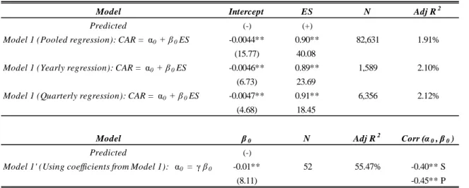
Panel A of table 5 presents benchmark regressions of 3-day announcement CARs
on earnings surprises in the range of -2 to +2 cents (Model 1) in the pooled, yearly and
quarterly regressions. Model 1 results, which are presented for unscaled surprises,
indicate that the intercept is significantly negative. As expected the ERC is higher than is
18
24
typically achieved for when the full range of earnings surprises is included in the
regression (Freeman and Tse 1992). The last row present the Spearman and Pearson
correlations between quarterly ERCs and intercepts and the coefficient from a regression
of quarterly intercepts on quarterly ERCs. Consistent with hypothesis 2, there is reliably
negative association.
In rational expectations models of reporting bias, the marginal benefit of a positive
surprise is increasing in the a priori level of a stock’s ERC. In contrast, it could be argued
(as some of the studies cited in section 2 do) that the realization of a positive surprises
leads to a higher ERCs. To date, no empirical study has discriminated the direction of
causality between the ERC and a surprise. However, either possibility suggests that there
will be a monotonic relation between PPS and ERC and, by hypothesis 2, a monotonic
relation (in the opposite direction) between PPS and the intercept. Panel B presents
intercepts and ERCs in pooled and yearly regressions by quintile ranks of PPS. There is
evidence of monotonicity in PPS for both parameters and in opposite directions.
One possibility raised by the findings reported in panel B is that when any variable
hypothesized to be linked to asymmetric price reactions to bright line surprises is
correlated with PPS, tests of the hypothesis that are based on differential ERCs can be
confounded. To assess the potential for correlated omitted variables, I augment Model 1
by adding the variable PPS and an interaction term PPS*ES and label this Model 2.
Results for unscaled ES in pooled and yearly regressions are presented in panel C of table
5. The results indicate that the PPS indicator is negative and highly significant while the
interaction PPS*ES is positive and highly significant in the pooled and yearly regressions.
25
the coefficient on PPS*ES is positive in 11 of 13 years. The results for Model 2 strongly
suggest that to the extent any variable used to partition data that is correlated with PPS
will likely contribute to a finding of asymmetric price reactions to bright line surprises
(see also section 5.1, footnote 23).
4.3. Robustness tests
4.3.1. Hindsight biases in surprises
The empirical tests conducted thus far rely on actual EPS and consensus analyst
forecast data obtained from IBES. According to Bradshaw and Sloan (2002), Abarbanell
and Lehavy (2007), IBES reports “street” earnings excluding one-time items (e.g., special
items) and, therefore, the size and sign of surprises measured with IBES data can differ
from the size and sign perceived by investors. In addition, Livnat and Mendenhall (2006)
report that IBES often chooses the components to include in reported EPS after observing
the market reaction to the earnings announcement. As discussed in the next section, even
if systematic biases and/or hindsight biases are introduced into IBES surprises by a data
provider’s administrative procedures, the hypotheses and results in the paper would still
be relevant, however, it would be difficult to attribute the results thus far to the empirical
validity of theories that posit a strategic incentive for managers to produce biased
surprises.
To ameliorate the effects of possible hindsight biases that contaminate tests of price
reactions to earnings surprises, I employ a proprietary dataset from Briefing.com that
should be free from this potential problem. Briefing.com provides real-time coverage of
26
outstanding First Call forecast consensus on the date of the earnings announcement. The
following excerpt from Briefing.com provides an example.
7:34AM CMS Energy beats by $0.06, reports revs in-line (CMS) 10.63 : Reports Q4
(Dec) earnings of $0.30 per share, excluding non-recurring items, $0.06 better than the
First Call consensus of $0.24; revenues rose 10.2% year/year to $1.84 bln vs the $1.84
bln consensus.19
I collect all available quarterly earnings announcement data from Briefing.com
using a text searching program, PERL, and construct a dataset of observations common
to IBES and Briefing.com with respect to the earnings announcement date. I then rerun
all of the key tests of this section. The total number of observations for this dataset is
25,886, considerably smaller than the original sample because Brieifing.com only began
extensive coverage of earnings announcements after 1997 and because I delete
observations for which the two data services do not report the same earnings
announcement date. Untabulated descriptive statistics indicate that, compared to the
sample used in this study, firms in this common dataset report larger EPS (mean of 41
cents versus 25 cents), total assets (mean of 8,207 million versus 3,127 million), earnings
surprises (2 cents versus -1 cents), and size-adjusted returns (mean 0.38% versus 0.18%).
However, the industry composition is very similar using the Fama-French 30 industry
classification.
I find that the Briefing.com sample produces results qualitatively similar to those
reported for the sample in tables 2-5 (untabulated for the sake of brevity). Specifically, I
27
find that the ratio of positive-to-negative surprises is increasing in PPS, zero surprises
produce negative stock reactions, on average, which are increasing in PPS quintile, and
the surprise necessary to produce a neutral stock reaction is significantly positive and
increasing in PPS quintile. I also find that the PPS is increasing in ERC and that ERCs
and intercepts in regressions of CAR on ES are negatively correlated.
4.3.2. Changing the cutoff used to define PPS
The logit model estimation of PPS described in the appendix is based on the
specification in Barton and Simko (2002), which estimates the probability that a surprise
will be greater than or equal to zero.20 Table 6 presents the PTN and CARs for zero
surprises by quintile of PPS for alternative cutoffs used to estimate PPS. The alternative
cutoffs range from -3, -2 -1, 0, +1, +2 and +3 cents. The results are qualitatively similar
for each alternative cutoff. In untabulated results I also find that intercepts are decreasing
and ERCs are increasing in PPS for all alternative specifications using these cutoffs. In
the next section I elaborate on these results and their implications for studies that
hypothesize that firms engage in deliberate efforts to manage earnings or analysts’
forecasts in an effort to meet or beat expectations.
5. Interpreting prior literature using a rational framework
5.1. Evidence of the existence of a “Torpedo” effect
Some studies hypothesize asymmetric price responses to bright line earnings
surprises for reasons that would have no direct implications for the actual empirical
distributions of earnings surprises. In other words, these theories do not predict a
28
propensity for positive earnings surprises in distributions of earnings surprises like that
observed in figure 1, but nevertheless employ such distributions in their empirical tests.
Moreover, inferences from empirical tests of these hypotheses often implicitly rely on the
neutral reaction assumption and/or are affected by the practice of partitioning data on ex
post realizations of surprises.
Some of the hypotheses that predict asymmetric price responses to surprises that
meet or fail to meet “bright lines,” link the prediction to either market mispricing or a
correction of prior mispricing. For example, following on Lakonishok, Shleifer and
Vishney (1994), Skinner and Sloan (2002) hypothesize that investors fixate on firms’ past
growth and maintain unreasonably high growth expectations for firms with high past
growth rates, i.e., firms with high market-to-book ratios or high price-to-earnings ratios.
They argue this irrationality is corrected around earnings announcements when there is a
negative earnings surprise. This in turn, results in larger negative stock price reactions to
small negative surprises for high MB and PE firms. Skinner and Sloan compare
announcement CARs of high and low MB (PE) firms for small positive and negative ex
post surprises and find that the difference in CARs for the latter are significantly larger in
absolute magnitude than that for the former. They deem this response the “Torpedo”
effect. 21
21Other theories posit rational but non-linear responses to small negative versus positive earnings surprises
29
Panel A of table 7 presents mean PPS, PTN and CAR at zero earnings surprises for
MB and PE and quintiles. All three variables are increasing in MB and PE, a result that
still holds when MB is not included in the estimation of PPS (see appendix 2). That is,
there is reason to suspect that PE and MB are also proxies for the ex ante probability of a
positive surprise. Similar to the results for PPS, differences in PTN and CAR for zero
surprises between the high and low quintiles are significant for both MB and PE.
Panel B of table 7 reports the three-day size-adjusted stock return for earnings
surprises ranging from -3 to +3 cents for all observations and by MB and PE quintile. As
predicted by the positive correlation between MB (PE) and PPS, the difference in mean
CARs between the highest and the lowest MB (PE) quintiles for surprises of -2 and -1
cent (-1 cent) are significantly larger in magnitude than mean CARs for surprises of +2
and +1 cents (+1 cent), respectively.22 That is, ignoring the negative CAR to zero
surprises (i.e., accepting the empirical validity of the neutral reaction assumption)
predicted in hypothesis 1a and empirical results on different ZEROs by PPS reported in
the previous section, then comparing returns to surprises of a similar magnitude on either
side of zero leads to the conclusion that price responses are asymmetrically more
negative for high MB (PE) firms for the negative earnings surprise. However, in
untabulated results when I estimate (out of sample) the value of a surprise that generates
a neutral response using the methods of interpolation and regression by MB quintile, I
find that the absolute value of the difference in CARs between high MB and low MB
22Note Skinner and Sloan (2002) use a longer window abnormal return in order to capture the stock price
30
firms around surprises in the neighborhood of 1 cent above and 1 cent below the
interpolated value are not significantly different. A similar absence of significance is
observed when PE is used to sort the observations. Thus, after controlling for the
propensity for positive surprises in the ES distribution I find no support for the presence
of a torpedo effect based on CAR tests in my sample.23
The remaining columns of panel B report evidence of near monotonicity in CARs
but different ZERO points as a function of MB and PE rank. The evidence mirrors the
results reported in panel A of table 4 for level of PPS.
5.2. Purported penalties to surprises that take on specific values
The usefulness of the rational expectations framework and its implications for tests
of the information content of bright line surprises using comparisons of ERCs is perhaps
best illustrated in the context of studies that claim to show that earnings surprises that
take on specific values create asymmetric or discontinuous price responses. A recent
example is Keung, Lin and Shih (2009) (KLS). The authors posit that investors have
learned over time about managers’ increasing tendency to bias earnings surprises through
earnings or forecast manipulation. Relying on the learning hypothesis, they predict that
earnings surprises in the interval [0, 1] cent will be increasingly “penalized” by the
market over time. In essence, KLS draw a bright line on both sides of the earnings
surprise. They compare ERCs for earnings surprises in the interval [0, 1] cent to ERCs
for surprises in adjacent intervals also defined by a 1 cent range (i.e., the intervals [-1, 0)
and (1, 2], etc) and find evidence that ERCs associated with surprises in the interval [0, 1]
23In untabulated results I find that ERCs are strongly increasing while intercepts are strongly decreasing in
31
are lower than surprises for both adjacent bins in the last of the three 5-year sub periods
they examine but not in the first two. Based on these results, the authors conclude that the
market has recently come to view an earnings surprise of exactly 0 or 1 cent as a red flag.
KLS base their prediction on a rational market, albeit one that is slow to learn. If
this is so, then the predictions in H1a and H2 should both apply. KLS report abnormal
returns to zero surprises are negative in each of the three sub periods they examine (see
table 1 of KLS), consistent with the evidence presented in table 3 discussed in the
previous section. In addition, they report abnormal returns to zero and one cent surprises
become increasingly more negative in the last two sub periods. Although at first blush
this results seems to be consistent with KLS’s learning hypothesis, a closer examination
of abnormal return patterns in adjacent surprises reveals that increasingly more negative
abnormal returns for the last two sub periods are observed for most of earnings surprises
ranging from less than -4 cents to 2 cents, which is inconsistent with KLS’s hypothesis
that zero and one cent are especially penalized by investors. Furthermore, they show that
abnormal announcement returns are monotonically increasing in the sign and size of
earnings surprises in every sub period, which is consistent with the results reported in
panel A of table 4. That is to say, KLS find no evidence that the CARs for surprises in
interval [0, 1] interrupt the usual pattern of monotonicity in bins that contain increasingly
larger ex post surprises. Of course, it is possible for CARs to follow a monotonic pattern
in ex post surprises while the ERCs associated with surprises in the interval [0, 1] are
lower than those associated with adjacent bins.
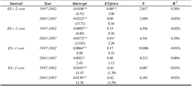
I test the possibility of lower ERCs for surprises in the [0, 1] by running separate
32
to +2 cents for the last two 5-year sub periods examined by KLS. The key difference
between my regression and KLS’s is that I allow intercepts to vary by bin while they do
not. In addition, I do not aggregate zero surprises with one cent surprises because there is
no variation in the independent variable for zero surprises. Scaling by price is required
because of the absence of variation in the independent variable in unscaled surprises.
The results of these regressions are shown in panel A of table 8. Unlike the results
in KLS, slope coefficients (i.e., ERCs) are never significant for any level of surprise in
either sub period once the intercepts are included. However, the y-intercept generally
decreases for the second sub periods for most intervals. This is consistent with the
presence of greater reporting bias in the second sub-period throughout a wide range of
earning surprises, which was also indicated by the results in panel B of table 2 and table 3.
That is, while not monotonically increasing over time larger negative reactions to small
surprises were observed on average in these years. Thus, inconsistent with KLS’s
hypothesis, the market seems to penalize all small earnings surprises, not just surprises of
zero or one cent. Furthermore, the penalty to these surprises appears through the average
abnormal return, not through the ERC.24
Panel B of table 8 presents regressions similar to those presented in panel A but
include the level of PPS as well as an interaction term between PPS and ES to test
hypothesis 2. These regressions tests a joint hypothesis implied by the rational
expectations framework. If investors penalize +1 cent earnings surprises by assigning
lower ERCs because they are more likely to be biased than other surprises, and if the
24
33
investors assess each firm’s possibility of the bias, then the PPS coefficient should be
positive while the PPS*ES coefficient should be negative in the second sub-period for +1
cent surprises. On the other hand, if investors penalize +1 cent earnings surprises by
assigning low average returns instead of low ERCs, then the PPS coefficient should be
negative while the PPS*ES coefficient should be positive in the second sub-period for +1
cent surprises. I find no evidence of an unusual penalty to +1 cent surprises in ERCs as
the interaction terms for all intervals are insignificant. Furthermore, the PPS coefficient
takes on mostly negative values for all intervals. These results indicate the penalty is
applied to high PPS firms in all surprise bins, however the penalty is applied through the
average stock return, in contrast to KLS’s hypothesis. I conclude that the absence of
significantly positive ERC interactions for most small surprises even in the presence of
significantly negative intercepts is attributable to the lack of meaningful variation in the
independent variables.
The evidence presented in table 8 suggests that tests for asymmetric price reactions
that compare the incremental slopes of adjacent bins without also controlling for the
propensity for a positive surprise and including incremental intercepts to capture the
effect predicted by hypothesis 1a or 2 will have low power and can result in incorrect
inferences. The argument is analogous to the discussion of potentially confounded
inferences when abnormal returns on either side of a bright line are compared but
generalized bias is present in all surprises.
34 5.3. The “Meet or Beat” literature
The notion that firms bias earnings or manage forecasts with the intent to “meet or
beat” analysts’ expectations (MBE) has gained greater credence with the growing number
of academic studies that presume or attempt to test the empirical validity of the claim
(Lopez and Rees 2002, Matsumoto 2002, Bartov et al. 2002, Kasznik and McNichols
2002, McVay, Nagar and Tang 2006, and Koh et al.2008). General acceptance of the
claim has been furthered by repeated anecdotes in the popular press and highly publicized
statements by policy makers concerned with what they term the “numbers game” (Levitt
1998). The increased attention to the MBE argument has, in turn, spawned a stream of
work that seeks to develop models that predict the ex ante probability that a firm will
report earnings with the specific intent of beating analysts’ expectations. Barton and
Simko (2002), Matsumoto (2002), Rees (2005) and Cheng (2006), for example, all
employ variations of the logit model describe in the appendix to estimate the ex ante
probability that a firm meets or beats expectations (PMBE).
However, the results in table 3 demonstrate zero earnings surprises generate, on
average, negative stock responses while small positive surprises generally produce
neutral or positive surprises. This evidence suggests the empirical definition of MBE,
which contemplates homogeneity of the market response to “on-cutoff” (i.e., zero
surprises) and “above-cutoff” (i.e., positive surprises) fails to account for the fact that the
former observations produce stock price reactions that are fundamentally different from
the latter. In addition, Barton and Simko (2002) show that the variables used to estimate
the MBE point in logit models perform similarly when the cutoff point selected for the