1Abstract—The mathematical model of load frequency control is established in the interconnected power system of hydro, thermal, and wind for solving the problem of frequency instability in this paper. Besides, the improved grey wolf optimization algorithm (GWO) is presented based on the offspring grey wolf optimizer (OGWO) search strategy to handle local convergence for the GWO algorithm in the later stage. The experimental results show that the improved grey wolf algorithm has a superior optimization ability for the standard test function. The traditional proportional integral derivative (PID) controller cannot track the random disturbance of wind power in the hydro, thermal, and wind interconnected power grid. However, the proposed OGWO dynamically adjusts the PID controller control parameters to follow the wind power random disturbance, regional frequency deviation, and tie-line power deviation.
Index Terms—Load frequency control; Area control error;
Hydro-thermal-wind interconnected power system; Improved grey wolf optimization algorithm.
I. INTRODUCTION
As the energy crisis becomes more and more serious, a large number of new energy sources, such as wind power, has an impact on the grid after being connected to it [1]. It brings about the frequency fluctuation of the grid. The load frequency control (LFC) is an important part of automatic power generation control (AGC). In the interconnected power grid, the varieties of power and frequency in some regions cause the fluctuation of tie-line power and consequently affect the stability of the entire interconnected power grid [2]. Therefore, load frequency control has been actively researched in different strategies, including the traditional proportional integral derivative (PID) control [3], auto-interference control [4], [5], optimal control [6], sliding mode control [7], robust control [8], [9], and adaptive control [10]. The best control strategy depends on the problem to be addressed. In addition, each strategy has different shortcomings, such that a linear model replaces the nonlinear control object mathematical model or the control effects are heavily dependent on the accuracy of model parameters, or
Manuscript received 12 August, 2020; accepted 11 October, 2020. This work was supported by National Natural Science Foundation of China under Grant No. 51167003 and by Guangxi Natural Science Foundation under Grant No. 2014GXNSFAA118320.
the controller cannot effectively restrain the random disturbance. Accordingly, the traditional PID controller is still widely used in most of the interconnected power grids.
With a significant advance in artificial intelligence algorithms, many intelligent algorithms were applied to load frequency control due to their robustness to parameters. Intelligent algorithms dynamically adjust the varied parameters of the PID controller in a suitable range through powerful search and iteration capabilities. Thus, the power grid has a stronger anti-interference ability, and the entire power system presents not bad dynamic performance. The hybrid method of genetic and particle swarm optimization (PSO) was proposed to eliminate frequency errors and suppress fluctuations in tie-line power for interconnected power grid [11]. In [12], the improved fruit fly optimization was proposed for interconnected power systems containing wind power and the frequency fluctuation. In [13], the firefly optimization algorithm was employed to revise the PID parameters to control the load frequency control of the multi-region interconnected power grid. In [14], [15], the GWO algorithm was used to adjust the controller parameters. The simulation results showed that the GWO algorithm could quickly suppress the power system frequency and power oscillation. However, in the later stage of the algorithm, the weight of the lead wolf becomes too large, so easy to fall into the local optimum. In [16], [17], the grey wolf algorithm was used to control and optimize multi-area load frequency control. However, it similarly faced the convergence problem. The proportion of the lead wolf became too large in the later stage, falling into local optima. In [18], the grey wolf optimization algorithm was used to optimize the load frequency control problem with time delay. In [19], the grey wolf algorithm with fixed weight showed a superior result in the optimal frequency control. However, the method led to slow convergence and low accuracy.
Those intelligent optimization strategies showed superior optimized control parameters than the traditional PID control strategy. However, the convergence accuracy and speed were different across different strategies. When a large frequency disturbance occurs in the power grid, the system should quickly increase the power generation or remove a specific load. In this paper, the model of a three-region interconnected power system with wind power is first established. Then, the
Multi-Area Load Frequency Control of
Hydro-Thermal-Wind Power Based on Improved
Grey Wolf Optimization Algorithm
Fannie Kong*, Jinfang Li, Daliang Yang
Department of Electrical Engineering, University of Guangxi, 530000, Nanning, Guangxi, China
actual data for wind farm power are integrated into the grid. The PID control parameters are optimized and regulated by the improved grey wolf algorithm based on offspring grey wolf optimizer (OGWO). The simulation results show that the improved grey wolf algorithm has a superior controlled performance response.
II. SYSTEM MODEL A. Load Frequency Control Model
Load frequency control is based on the control error of each area to achieve the control and adjustment of the generator units. By adjusting the active power output of the generator units, the frequency fluctuations between the areas
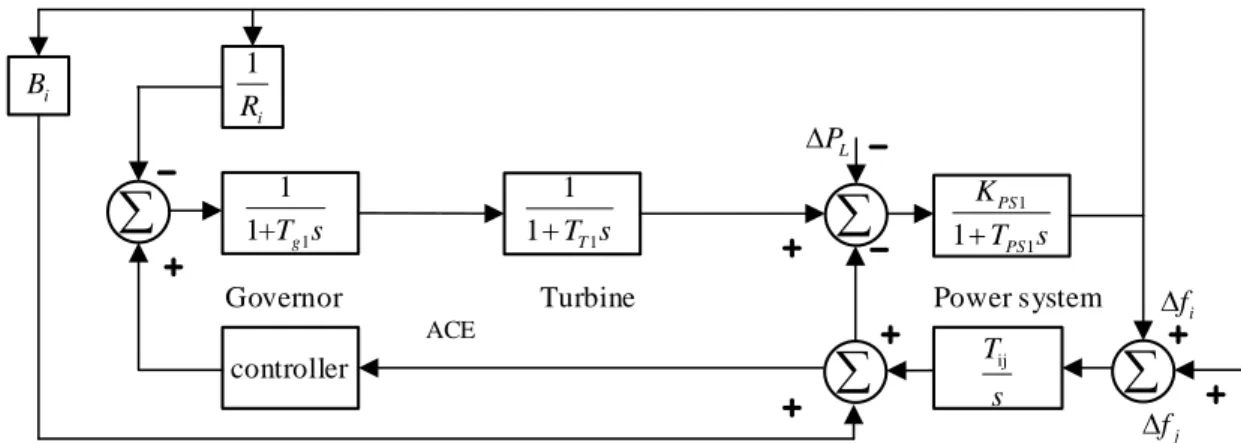
are decreased so that the regional control error will pass zero after a while to ensure the stability of the entire system. This paper constructs the model for three areas with hydro, thermal, and wind power. The IEEE standard mathematical model for hydro and thermal power used in this paper is composed of the governor, water turbine, steam turbine, and generator individually. The schematic diagrams of load frequency control models for thermal- and hydro-powers are shown in Fig. 1 and Fig. 2 [14]–[19].
As shown in Fig. 1, the model for thermal power is composed of a steam turbine governor, steam turbine, and synchronous generator. Tg1 is the steam turbine governor time
constant; TT1 is the steam turbine time constant; Kps1 is the
generator gain coefficient; Tps1 is the generator time constant.
controller i B 1 i R ij T s
Governor Turbine Power system
1 1 1+T sg 1 1 1T sT 1 1 1 PS PS K T s
ACE i f j f L P Fig. 1. Load frequency control model for thermal power.
controller 2 2 1 PS PS K T s
i B 1 i R 1 1T ss 2 1 1 R T s T s ij T s w w 1 s 1+0.5 T T s Governor Hydroturbine Power system
ACE fi L P j f Fig. 2. Load frequency control model for hydropower.As shown in Fig. 2, the model for the hydropower is composed of a speed governor with a compensator, turbine, and synchronous generator. Ts is the time constant of the
governor; TR, T2 are the time constants of the turbine control
valve; TW is the start-up time of water; Kps2 is the generator
gain coefficient; Tps2 is the generator time constant; Δfi is the
frequency deviation; Ri is the governor adjustment
coefficient; Bi is the area frequency deviation coefficient; Tij
is the tie-line power synchronization factor.
In Fig. 1 and Fig. 2, area control error (ACE) is the area control deviation, mainly composed of frequency and tie-line power deviation. It is defined as follows
Δ ij Δ ,
tie i
ACE = P + k f (1)
where Δfi is the area frequency deviation, and ΔPtie is the
tie-line power deviation between different areas. k is the control area deviation coefficient.
The structure of a PID controller is depicted in Fig. 3.
i K d K du dt 1 s p K ACE u
Fig. 3. The structure of PID.
The u1-u2 are the output of the PID controller defined by
following equations:
, p i d dACE u K ACE K ACE dt K dt
1 1 1 1 1 1 + 1 (2) 2 2 p2 1 i2 2 d2 dACE u = K ACE + K ACE dt + K . dt
(3)The control parameters of PID controller KP1-KP2, Ki1-Ki2,
and Kd1-Kd2 are selected by three different algorithms:
OGWO, GWO, and PSO, respectively. B. Wind Power Generator Model
For wind power generator, wind speed is the main parameter that affects the power output. The randomly varied wind speed causes the instability of generator output power; consequently, it affects the frequency of the system. At present, the four-component model is often used in the wind energy model. It comprises of basic wind, gust wind, gradual wind, and arbitrary wind [20].
The wind energy is converted into mechanical energy by the wind generator. The output power is defined as
3 1 , 2 W P P = ρSv C (4)
where Pw is the output mechanical power of the wind turbine.
CP is the utilization factor of wind energy, and the typical
value is CP = 0.593. S is the active area by the wind turbine,
and v is the wind speed.
III. GWOALGORITHM
An intelligent optimization search algorithm, GWO, was first proposed in [21]. The optimization process mainly includes the following steps.
A. Social Hierarchy System
The lead wolf is composed of three wolves α, β, and δ, whose characters are responsible for assigning the moving direction to the wolf ω. The wolf ω is mainly responsible for finding the optimal target solution and providing feedback to the head wolf simultaneously.
B. Surrounding Prey
After getting the instructions of wolf α, β,and δ, the wolf ω begin to surround its prey (optimum solution).The calculation method is modelled by following equations:
( ) ( ) ,
P
D = CX t - X t (5)
1 P ,
X(t + )= X (t)- A D (6)
where t is the number of iterations, A and C are coefficient vectors. XP(t) is the direction vector of the current target. X(t)
and X(t + 1) are the current position vector and the next moving direction vector. The coefficient vectors A and C are expressed as follows: 1 2 , A a r a (7) 2 2 , C r (8)
where a is linearly reduced from 2 to 0 as the number of iterations increases. The norm of r1 and r2 is a random
variable between [0, 1]. C. Attacking Prey
When the wolf group has been determined where is the location of prey, the α, β,and δ wolf lead the wolf group to surround the prey. These equations for position updating are shown as follows: 1 ( ) ( ) , D C X t X t (9) 2 ( ) ( ) , D C X t X t (10) 3 ( ) ( ) , D C X t X t (11) 1 1 , X X A D (12) 2 2 , X XA D (13) 3 3 , X XAD (14) 4( 1) 1 2 3/3, X t X X X (15)
where Dα, Dβ, and Dδ are direction vectors of wolves α, β, and
δ. X1, X2, and X3 are the next step moving direction vectors of
the wolf ω following wolves α, β, and δ.X4 is the final grey
wolf position.
During searching for the optimal goal, the lead wolf provides the individual with information about the intended target. However, only a few individuals play a role in the later period, and thus it is easy to fall into the local optima making the convergence slow. In order to overcome the problem, the offspring wolf is introduced in this paper. The algorithm of the final offspring grey wolf position is defined as in (16), (17), and (18). This improved strategy can further enhance the leadership ability of the wolves α, β, and δ and make the convergence fast. In addition, the local optima could be avoided to a certain extent. The calculation method is defined by following equations: min( ) min( ( )), { , , }, f X f X X X X1 2 X3 (16) min min min , ( ) ( ), ( ) , ( ) ( ), , ( ) ( ), X f X f X X t X f X f X X f X f X 1 1 5 2 2 3 3 (17)
, X6 t1 X5 t 1 X4 t (18) where the left side is the position of the final offspring grey wolf, (0, 0.5). In order to further verify the performance of the OGWO algorithm, a single-peak test function F1 and amulti-peak test function F2 are introduced. They are defined
as in (19) and (20): ( ) i , i F x1
x2 1 (19) ( ) i i cos( i ) . F x2
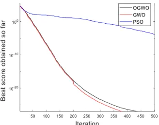
1x210 2x 10 (20) The test results on the conditions of x∈(-100, 100) in (19) and x∈(-5.12, 5.12) in (20) are shown in Fig. 4 and Fig. 5, where the iterative optimization of F1 and F2 are given,respectively.
As shown in Fig. 4 and Fig. 5, OGWO converged faster with high accuracy than GWO and PSO, proving the ability of OGWO in searching.
Fig 4. Convergence curves of OGWO, GWO, and PSO for test function F1.
Fig 5. Convergence curves of OGWO, GWO, and PSO for test function F2.
D. LFC Performance Index
The performance index of the system is mainly related to
the dynamic performance of the system, such as maximum overshoot, steady-state error, and rise time. Generally, the ITAE model can be selected as the performance index of the controller. Its definition is as follows
0 ( ) ,
ITAE
t e t dt (21)where the error e(t) is composed of frequency and tie-line deviations in the interconnected power system or ACE. In order to minimize the area control error, the frequency deviation and tie-line power deviation among different regions should be minimized. This can determine the performance index function of the LFC in this paper
, T ij i j tie J
f f P tdt 0 (22)where J is the performance index of LFC and T is integration time.
IV. CASE STUDY
In the actual power system, wind power is generally added to the interconnected power system as a disturbance source. The three-area interconnected power system composed of hydro, thermal, and wind power is researched in this paper as shown in Fig. 6. Area 1 is the IEEE standard thermal power unit, area 2 is the IEEE standard hydropower unit, and area 3 is the wind power. This is already described in Figs. 1 and 2 above. The used simulation parameters are as follows [14]–[19]: Tg1 = 0.08 s; Ts = 0.2 s; TT1 = 0.3 s; TR = 0.6 s; T2 = 5s; Kps1 = 120 Hz/p.u.MW; Kps2 = 75 Hz/p.u.MW; Tps1 = 20 s; Tps2 = 10 s; R1 = 2.4; R2 = 3.0; Tij = 0.545; B1 = 0.425; B2 = 0.425. controller controller
12 T s 2 1 1T sg
w pw 1 1 1T sg 1 1 1T sT 1 1 1 PS PS K T s Step 2 1 1T sT 2 2 1 PS PS K T s 2 B 2 1 R 1 1 R 1 B 2 1+ 1 R T s T s Fig 6. Three-area interconnected power.
V. RESULTS AND DISCUSSION
Without considering wind power, 10 % step load disturbance is exerted to the thermal power of area 1. PSO, GWO, and OGWO algorithms are applied to optimize the PID controller for balancing the area power grid. The
adjusting course curve of frequency deviation, ACE, and tie-line deviation of each area are shown in Figs. 7–12. In these mentioned figures, the red lines indicate the response of the OGWO based PID controller equipped power system; the blue line illustrates the response of the GWO based PID controller equipped power system, and the black line 35
indicates the response of the GWO based PID controller equipped power system.
The performance of OGWO is quantitatively compared with GWO and PSO in terms of the dynamic performance indexes and PID controller parameters in Table I and Table II.
TABLE I. PID CONTROLLER PARAMETER SETTINGS AND ITAE VALUE.
OGWO GWO PSO
Kp1 0.9934 0.9963 0.9911 Kp2 0.9564 0.9914 0.9956 Ki1 0.3234 0.3211 0.3196 Ki2 0.3699 0.3564 0.3711 Kd1 0.5169 0.5364 0.5456 Kd2 0.4175 0.4670 0.4943 ITAE 4.99 5.45 6.95
TABLE II. DYNAMIC RESPONSE VALUE OF DIFFERENT CONTROL AREA.
Settling time Peak overshoot/(10-1)
PSO GWO OGWO PSO GWO OGWO
Δf1 70.1 40.3 35.2 0.6178 0.2119 0.1007
Δf2 67.0 45.8 44.2 0.0191 0.0152 0.0112
ΔPtie 43.2 42.9 41.8 0.0473 0.0386 0.0250
ACE1 26.7 24.5 23.9 1.0711 0.8016 0.7663
ACE2 28.3 26.2 25.1 0.0578 0.5001 0.0476
Fig 7. Frequency deviation of thermal power area.
Fig. 8. Area control error of thermal power area.
Fig. 9. The frequency deviation of hydropower area.
Fig. 10. Area control error of hydropower area.
Fig. 11. The line power deviation.
When the step disturbance was exerted to the system, the PID controller parameters were optimized by the PSO, GWO, and OGWO algorithms. It is clear show in Figs. 7–11 and Table II that the OGWO algorithm optimized PID controller equipped power system achieved the least damping oscillations with the faster settled response, in addition to the minimal overshoot peak. Thus, it provided a superior controlled performance response compared to using GWO and PSO based PID controller equipped power system.
As shown in Fig. 11,under the disturbance of step signal, the traditional grey wolf optimization algorithm falls into local optimum after five iterations. It starts to jump out from 36
the local optimum after twenty-five iterations. The improved grey wolf optimization algorithm quickly reaches the optimal value at the beginning of the disturbance. As shown in Table I, minimum ITAE value is attained (4.99) using OGWO in comparison to GWO (5.45), and PSO (6.95). It is proved that the improved grey wolf algorithm can jump out from a local optimum quickly and consequently converge faster.
Fig. 12. Convergence curves of OGWO, GWO, and PSO.
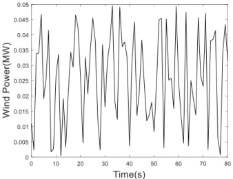
Taking into account the arbitrary nature of the wind, the disturbance source is supposed as the gust and random as shown in Fig. 13. PSO, GWO, and OGWO algorithms are applied to optimize the PID controller for balancing the area power grid. The curves of frequency and tie-line deviation are shown in Figs. 14–17.
Fig. 13. The wind power load disturbance.
When gust and random wind power are injected into the system, the system frequency deviation and tie-line power deviation become large. This is because wind power heavily affects the system and the system regulator cannot quickly adjust. The requirements of a stable system are satisfied when the frequency fluctuation of the system is between ± 0.5 Hz, and the fluctuation of the exchange power of the tie-line is between ±0.01 p.u. Although no algorithm can guarantee that the system frequency and tie-line power fluctuations are within the stable range, the OGWO is superior to GWO and PSO in control.
Fig. 14. The frequency deviation with gust power fluctuation.
Fig. 15. The line power deviation with gust power fluctuation.
Fig. 16. The frequency deviation with random wind power fluctuation.
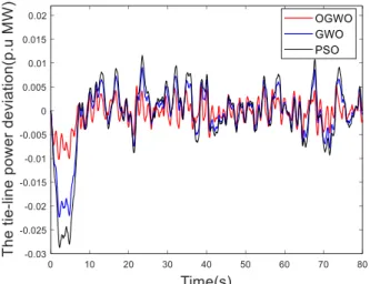
In Fig. 14 and Fig. 15, the proposed OGWO algorithm based controller can effectively reduce the peak undershoot and provide fast settled response compared to GWO and PSO based controller performance in the same investigated power system. As shown in Fig. 16 and Fig. 17 and Table III, the frequency and tie-line deviation are reduced to a smaller range (±0.03, ±0.01) to ensure the frequency stability of power system.
As shown in Fig. 18, the improved grey wolf optimization algorithm falls into local optimum after three iterations and jumps out from the local optimum until the 20th iteration.
The improved grey wolf optimization algorithm also falls 37
into local optimization in the optimization process, but it can escape quickly.
Fig. 17. The line power deviation with random wind power fluctuation.
Fig. 18. OGWO, GWO, and PSO convergence curves.
TABLE III. THE FREQUENCY AND TIE-LINE DEVIATION RANGE AND CONVERGENCE VALUE.
Frequency deviation range Tie-line deviation range ITAE OGWO ±0.03 ±0.01 46.4392 GWO ±0.06 ±0.025 55.3214 PSO ±0.05 ±0.03 57.3164
As show in Table III, minimum ITAE value is attained (46.4392) using OGWO in comparison to GWO (55.3214), and PSO (57.3164). From the view of the power system, smaller frequency and tie-line deviations can be obtained.
VI. CONCLUSIONS
The proposed work studied and developed a load frequency control of three-area interconnected hydro-thermal-wind power system by considering PID controller. The controller parameters, namely the proportional (KP), integral gain (Ki), and derivative gain (Kd),
are tuned by OGWO considering 10 % step load perturbation in area 1. The performance of proposed algorithm was compared to both the traditional grey wolf optimization algorithm (GWO) and the particle swarm optimization (PSO) technique based PID controller response. The superiority of the improved grey wolf optimization
algorithm was tested with different load disturbances. Finally, the simulation result obviously demonstrated that the OGWO algorithm tuned PID controller gained superiority (less damping oscillations, minimal settling time with less peak overshoot) compared to using the GWO and PSO tuned controller performances.
CONFLICTS OF INTEREST
The authors declare that they have no conflicts of interest. REFERENCES
[1] Y. Liu, Y. Chi, W. Wang, and H. Dai, “Impacts of large scale wind power integration on power system”, in Proc. of 2011 4th International Conference on Electric Utility Deregulation and Restructuring and Power Technologies (DRPT), Weihai, Shandong, 2011, pp. 1301–1305. DOI: 10.1109/DRPT.2011.5994096. [2] H. K. Shaker, H. El Zoghby, M. E. Bahgat, and A. M. Abdel-Ghany,
“Advanced control techniques for an interconnected multi area power system for load frequency control”, in Proc. of 2019 21st International Middle East Power Systems Conference (MEPCON), Cairo, Egypt, 2019, pp. 710–715. DOI: 10.1109/MEPCON47431.2019.9008158.
[3] A. Annamraju and S. Nandiraju, “Load frequency control of an autonomous microgrid using robust fuzzy PI controller”,in Proc. of 2019 8th International Conference on Power Systems (ICPS), Jaipur, India, 2019, pp. 1–6. DOI: 10.1109/ICPS48983.2019.9067613. [4] F. Liu, Y. Li, Y. Cao, J. She, and M. Wu, “A two-layer active
disturbance rejection controller design for load frequency control of interconnected power system”, IEEE Transactions on Power Systems, vol. 31, no. 4, pp. 3320–3321, Jul. 2016. DOI: 10.1109/TPWRS.2015.2480005.
[5] Md. M. Rahman and A. H. Chowdhury, “Parameterization of active disturbance rejection controller for load frequency control”, in Proc. of 8th International Conference on Electrical and Computer Engineering, Dhaka, 2014, pp. 552–555. DOI: 10.1109/ICECE.2014.7026976.
[6] N. Ch. Patel, M. K. Debnath, D. P. Bagarty, and P. Das, “Load frequency control of a non-linear power system with optimal PID controller with derivative filter”, in Proc. of 2017 IEEE International Conference on Power, Control, Signals and Instrumentation Engineering (ICPCSI), Chennai, 2017, pp. 1515–1520. DOI: 10.1109/ICPCSI.2017.8391964.
[7] Y. Mi, Y. Fu, Ch. Wang, and P. Wang, “Decentralized sliding mode load frequency control for multi-area power systems”, IEEE Transactions on Power Systems, vol. 28, no. 4, pp. 4301–4309, Nov. 2013. DOI: 10.1109/TPWRS.2013.2277131.
[8] H. Bevrani, Y. Mitani, and K. Tsuji, “Robust decentralised load-frequency control using an iterative linear matrix inequalities algorithm”, IEE Proceedings - Generation, Transmission and Distribution, vol. 151, no. 3, pp. 347–354, May 2004. DOI: 10.1049/ip-gtd:20040493.
[9] D. Rerkpreedapong, A. Hasanovic, and A. Feliachi, “Robust load frequency control using genetic algorithms and linear matrix inequalities”, IEEE Transactions on Power Systems, vol. 18, no. 2, pp. 855–861, May 2003. DOI: 10.1109/TPWRS.2003.811005.
[10] H. A. Yousef, K. AL-Kharusi, M. H. Albadi, and N. Hosseinzadeh, “Load frequency control of a multi-area power system: An adaptive fuzzy logic approach”, IEEE Transactions on Power Systems, vol. 29, no. 4, pp. 1822–1830, Jul. 2014. DOI: 10.1109/TPWRS.2013.2297432.
[11] C.-F. Juang and C.-F. Lu, “Load-frequency control by hybrid evolutionary fuzzy PI controller”, IEE Proceedings - Generation, Transmission and Distribution, vol. 153, no. 2, pp. 196–204, Mar. 2006. DOI: 10.1049/ip-gtd:20050176.
[12] J. Han, P. Wang, and X. Yang, “Tuning of PID controller based on Fruit Fly Optimization Algorithm”, in Proc. of 2012 IEEE International Conference on Mechatronics and Automation, Chengdu, 2012, pp. 409–413. DOI: 10.1109/ICMA.2012.6282878. [13] K. Jagatheesan, B. Anand, S. Samanta, N. Dey, A. S. Ashour, and V.
E. Balas, “Design of a proportional-integral-derivative controller for an automatic generation control of multi-area power thermal systems using firefly algorithm”, IEEE/CAA Journal of Automatica Sinica, vol. 6, no. 2, pp. 503–515, 2019. DOI: 10.1109/JAS.2017.7510436.
[14] D. Guha, P. K. Roy, and S. Banerjee, “A maiden application of modified grey wolf algorithm optimized cascade tilt-integral-derivative controller in load frequency control”, in Proc. of 2018 20th National Power Systems Conference (NPSC), Tiruchirappalli, India, 2018, pp. 1–6. DOI: 10.1109/NPSC.2018.8771738.
[15] A. Dogan, “Load frequency control of two area and multi source power system using grey wolf optimization algorithm”, in Proc. of 2019 11th International Conference on Electrical and Electronics Engineering (ELECO), Bursa, Turkey, 2019, pp. 81–84. DOI: 10.23919/ELECO47770.2019.8990643.
[16] M. K. Debnath, T. Jena, and R. K. Mallick, “Novel PD-PID cascaded controller for automatic generation control of a multi-area interconnected power system optimized by grey wolf optimization (GWO)”, in Proc. of 2016 IEEE 1st International Conference on Power Electronics, Intelligent Control and Energy Systems (ICPEICES), Delhi, India, 2016, pp. 1–6. DOI: 10.1109/ICPEICES.2016.7853271.
[17] D. Guha, P. K. Roy, and S. Banerjee, “Load frequency control of interconnected power system using grey wolf optimization”, Swarm
and Evolutionary Computation, vol. 27, pp. 97–115, 2016. DOI: 10.1016/j.swevo.2015.10.004.
[18] M. R. Shakarami and I. Faraji Davoudkhani, “Wide-area power system stabilizer design based on Grey Wolf Optimization algorithm considering the time delay”, Electric Power Systems Research, vol. 133, pp. 149–159, 2016. DOI: 10.1016/j.epsr.2015.12.019. [19] B. P. Sahoo and S. Panda, “Improved grey wolf optimization
technique for fuzzy aided PID controller design for power system frequency control”, Sustainable Energy, Grids and Networks, vol. 16, pp. 278–299, 2018. DOI: 10.1016/j.segan.2018.09.006.
[20] Sh. Yang-Wu et al., “Load frequency control strategy for wind power grid-connected power systems considering wind power forecast”, in
Proc. of 2019 IEEE 3rd Conference on Energy Internet and Energy System Integration (EI2), Changsha, China, 2019, pp. 1124–1128. DOI: 10.1109/EI247390.2019.9062084.
[21] Ch. Yan, J. Chen, and Y. Ma, “Grey wolf optimization algorithm with improved convergence factor and position update strategy”, in Proc. of 2019 11th International Conference on Intelligent Human-Machine Systems and Cybernetics (IHMSC), Hangzhou, China, 2019, pp. 41–44. DOI: 10.1109/IHMSC.2019.00018.
This article is an open access article distributed under the terms and conditions of the Creative Commons Attribution 4.0 (CC BY 4.0) license (http://creativecommons.org/licenses/by/4.0/).