Extending a Consensus-based Fuzzy Ordered Weighting Average (FOWA) Model in New Water Quality Indices

824

Extending a Consensus-Based Fuzzy Ordered Weighting Average (FOWA)

Model in New Water Quality Indices

Mohammad Ali Baghapour

, Mohammad Reza Shooshtarian

1) Research Center for Health Sciences, Institute of Health, Shiraz University of Medical Sciences, Shiraz, Iran

2) Department of Environmental Health Engineering, School of health, Shiraz University of Medical Sciences, Razi St, Shiraz, Iran

*Author for Correspondence:[email protected]

Received: 16 Jan. 2016, Revised: 10 March 2017, Accepted:07 May.2017

ABSTRACT

In developing a specific WQI (Water Quality Index), many quality parameters are involved with different levels of importance. The impact of experts’ different opinions and viewpoints, current risks affecting their opinions, and plurality of the involved parameters double the significance of the issue. Hence, the current study tries to apply a consensus-based FOWA (Fuzzy Ordered Weighting Average) model as one of the most powerful and well-known Multi-Criteria Decision- Making (MCDM) techniques to determine the importance of the used parameters in the development of such WQIs which is shown with an example. This operator has provided the capability of modeling the risks in decision-making through applying the optimistic degree of stakeholders and their power coupled with the use of fuzzy numbers. Totally, 22 water quality parameters for drinking purposes were considered in this study. To determine the weight of each parameter, the viewpoints of 4 decision-making groups of experts were taken into account. After determining the final weights, to validate the use of each parameter in a potential WQI, consensus degrees of both the decision makers and the parameters are calculated. The highest and the lowest weight values, 0.999 and 0.073 respectively, were related to Hg and temperature. Regarding the type of consumption that was drinking, the parameters’ weights and ranks were consistent with their health impacts. Moreover, the decision makers’ highest and lowest consensus degrees were 0.9905 and 0.9669, respectively. Among the water quality parameters, temperature (with consensus degree of 0.9972) and Pb (with consensus degree of 0.9665), received the highest and lowest agreement with the decision-making group. This study indicated that the weight of parameters in determining water quality largely depends on the experts’ opinions and approaches. Moreover, using the FOWA model provides results accurate and closer- to-reality on the significance of each of the water quality parameters. Thus, using this operator can be a precise and appropriate method to determine the parameters’ weights and importance in order to develop specific WQIs for drinking, industrial, and agricultural purposes.

Key words:

LIST of ABBREVIATIONS

WQI: (Water Quality Index)

NSFWQI: (National Sanitation Foundation Water Quality Index) MCDM: (Multi Criteria Decision Making)

GFDM: (Group Fuzzy Decision Making) AHP: (Analytical Hierarchy Process) SAW: (Simple Additive Weighting)

FOWA: (Fuzzy Ordered Weighting Average)

TOPSIS: (Technique for Order Preference by Similarity to Ideal Solution) RIM: (Regular Increasing Monotonous)

DM: (Decision Maker)

INTRODUCTION

Many environmental and health legislator institutions have used different water quality parameters as applicable and useful criteria to develop WQIs. The advantage of these indices is aggregating the

825 specific place in water resources management plans, especially in drinking section [4, 5]. So far, many global WQIs have been introduced for evaluating the water quality, but they may not be properly useful for all regions. Many researchers also believed that these indices are not appropriate to be used universally due to consideration of professionals’ opinions in specific regions of the world and improper distribution of the parameters’ weights [6-8]. Hence, developing specific and local WQIs has been welcomed in recent years. For instance, Prakirake et al., [9], developed a specific WQI for rivers in Thai region in Thailand, 2009. In order to determine parameters’ weights, they used the Delphi technique just like the NSFWQI method, but through benefiting from 24 experts’ opinions in Thailand. They selected and weighted 13 parameters, including turbidity, Fe, fecal coliforms, TDS, NO3, pH, DO, color, NH3, Mn, BOD5, total hardness, and total phosphorus.

Generally, the process of developing a standard WQI includes different stages, such as selecting and weighting the parameters, determining the sub-index of each parameter, and aggregating them to calculate the index value [10]. Among these stages, the weighting process is considered to be one of the most important and determinant ones. This process is affected by many factors, such as parameters type, water consumption, local standards, intensity of the resulting impacts due to their increased concentration, accessibility to water treatment facilities, and decision makers’ viewpoints, knowledge, and experiences. These factors lead to uncertainty and more complexity in the weighting process. Due to such ambiguities, in spite of the need for specifying WQIs by considering local conditions, many societies are still using conventional indices. These problems indicate the necessity to use accurate and powerful ways. Using MCDM techniques can be considered to be an appropriate way to solve such problems. These models have indicated a high potential in water resources management and environmental assessment [11]. In the recent years, researchers have benefitted from MCDM methods for weighting parameters in local WQIs. In 2012, Karbassi et al. [12], developed a specific WQI for Gorgan Rood River, Iran. They considered nine parameters, including pH, temperature deviation, PO4, NO3, DO, BOD5, fecal coliforms, turbidity, and TSS. Then, they weighted the parameters using the AHP method. In 2013, Kohanestani et al., [13], used the AHP model to weigh 9 parameters in order to evaluate the water quality in Zaringol Stream in Golestan Province, Iran.

Fuzzy theory is a robust way to deal with uncertainties in the weighting process. If this theory is used appropriately, it can be a useful tool to assess

environmental problems, Raman believes. This method, then, has been used by researchers for solving the complexities of issues in the field of water, especially when a large number of parameters are involved in water quality. Studies of hosseini-moghari et al., 2015, Kageyama et al., 2016, and Tavakoli et al., 2015 are some new researches in this field [14-19] . FOWA operator is one of the most powerful MCDM methods, which can model the risks and uncertainties in aggregating group opinions. On the other hand, very rarely applied researches about water quality issues have been conducted using this model. Therefore, the present study aimed to evaluate application of a consensus-based Fuzzy OWA model to determine water quality parameters’ weights in order to utilize them in specific WQIs which was illustrated as a case study.

MATERIALS AND METHODS

Background information

Fuzzy numbers

The infrastructure of fuzzy theory was developed by Zadeh in 1965. It was then established by Zadeh and Bellman in 1970. In recent years, increasing attention has been paid to utilization of this theory for analyzing and controlling complex systems. This is due to the fact that it is capable of being understood by humans and is considered to be a successful method in modeling non-linear functions based on the natural language [14, 20]. Fuzzy numbers are used for utilizing linguistic terms and considering uncertainties. If X is a non-empty set, the fuzzy set A in X is expressed as its membership function:

[ ]

Where μ_A (x) is interpreted as the membership degree of the element X in the fuzzy set A so that x ϵ X.

A fuzzy number like A is known by its membership function μ_A (x), which depends on each x of A as a real number. Membership functions of fuzzy numbers are expressible in triangular, trapezoidal, or Gaussian (bell shape) layouts. The examples of these functions are shown in Fig. 1. Triangular fuzzy numbers were used in the MCDM model in the present study.

826 A triangular fuzzy number is expressed as Eq. 1:

( )

{

( )

( ) ( )

( )

Eq(1)

Arithmetic functions in a triangular fuzzy number are as follows:

{

( ) ( )

( ) ( ) ( )

( _{( ) ( )}

Eq (2)

FOWA operator

OWA operator is one of the well-known MCDM models, which was extended by Yager in 1988. Thereafter, introducing the fuzzy theory in the model was an appropriate response to uncertainties in group decision making problems [20]. In order to approximate the decision- making process to real conditions and apply stakeholders’ opinions,

measures such as existing risks, including DMs’ optimistic and pessimistic views, as well as their power have been considered. Indeed, OWA method is a mapping of an n-dimensional to one-dimensional space in which, according to Eq. 3, there is a dependent weight vector of wj:

( ) ∑ Eq(3)

is the jth value in input dataset { }. In fact, vector b indicates the descending ordered values of the vector a, which are indeed the weight of a criterion from the viewpoint of each DM. In this equation, n is the number of DMs. shows the order weight and has the following conditions:

∑ Eq (4)

Optimistic degree

With changes in the orders’ weights, the OWA operator’s behavioral features change, as well. The orders’ weight change in this operator reflects DMs’ optimistic or pessimistic attitude. Larger values at the beginning and at the end of the vector of the orders’ weight indicate DMs’ optimistic and pessimistic attitude towards the issue, respectively. For modeling this feature, the term optimistic degree (θ) was introduced by Yager in 1988 as Eq. 5:

𝛉 ⁄ ∑ ( ) Eq (5)

Where, n is the number of criteria.

The value ranges from zero to 1. In addition, it can be defined through three modes as is shown in Fig.2.

Fig. 2: Different statuses for optimistic degree (20)

In this study, a fuzzy linguistic quantifier namely RIM operator was used to extract the orders’ weights (w_j). In this quantifier, linguistic terms are expressed by the fuzzy membership function of Q(r) in the range of. Eq. 6 is one of such quantifiers that has many applications in this regard:

( ) Eq (6)

In the current study, the strictly RIM operator was used according to eq. 9. Assuming that n → ∞, and merging Eq. 5 and Eq. 6, we have:

θ ∫

⁄

Eq (7)

The linguistic quantifiers and their equivalentθ are presented in Table 1.

Table 1: Family of RIM and its relevant θ values [20]

Optimism degree Optimism

status Parameter of

the quantifier Linguistic

quantifier

0.999

At least one of

them

0.909 Optimistic

0.1

Few of them

0.667 0.5

Some of them

0.500 Neutral

1.0

Half of them

0.333 2.0

Many of them

0.091 Pessimistic

10.0

Most of them

0.001

∞

All of them

Based on the optimistic degree, Eq. 3 can be defined as Eq. 8:

( ) ∑ [( ) ( ) ] Eq (8)

827

DM’s power

This term indicates the value of each stakeholder’s opinion about the criteria’s importance. Since DMs’ power has been defined by using linguistic terms, the fuzzy linguistic quantifiers in Table 2 should be utilized in order to change them into fuzzy numbers and use them in the model.

Table 2: Fuzzy numbers for DMs’ power [22]

Fuzzy numbers Label

Linguistic variables

(0.00, 0.00, 0.01) VL

Very low

(0.2, 0.10, 0.20) L

Low

(0.35, 0.20, 0.20) SL

Slightly low

(0.50, 0.20, 0.20) M

Medium

(0.65, 0.20, 0.20) SH

Slightly high

(0.80, 0.20, 0.10) H

High

(1.00, 0.10, 0.00) VH

Very high

If the numeric value of the jth criterion’s weight from the viewpoint of is equal to ( ), the value of the criterion’s weight with applying each DM’s power can be computed using Eq. 9: ( )

( ( ) ( ) ( )) Eq(9)

Consensus degree

In group decision problems, all stakeholders’ consensus on the criteria must be taken into account. This term indicates that only the criteria with the minimum agreement from DMs should be used in the decision-making process. According to Ashton’s remark in 1992, the minimum consensus threshold to accept the results of group opinions is 0.6 [23]. To determine this measure, first the non-consensus degree of each stakeholder is defined based on Eq. 10

:

( ) | ( ) ( )| Eq (10) Where ( ) is, the non-consensus index, ( ) is the DM’s opinion regarding the weight of criterion j, and ( ) is the numerical value of the group’s opinion on the importance of the criterion j (group weight of criteria j). In this study, the value of p is supposed to be equal to 1. The consensus degree of the criteria is calculated according to Eq. 11:

(

₎

⁄ ∑

(

)

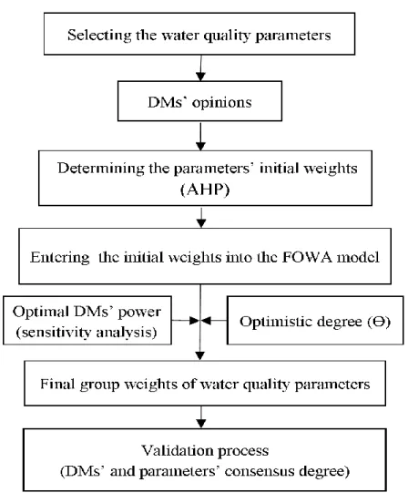
The proposed methodology

The proposed MCDM framework is shown in Fig. 3. In a WQI, lots of water quality parameters are

involved with different levels of importance. In the process of developing new WQIs, stakeholders’ opinions should be considered in a proper way to determine parameters’ weights. In this framework DMs’ viewpoint regarding each parameter’s importance is taken by using pairwise comparison matrix of AHP. Besides, initial weights are calculated using Expert Choice software. The consensus-based FOWA model consists of a group decision making section. By applying optimistic degree and DMs’ power, this model is used to aggregate group’s opinions and finalize parameters’ weights. After calculating the final weights of water quality parameters, they should be validated in order to make sure that they have received the minimum agreement from DMs. It should be considered by determining the consensus degree of each parameter. Generally, changes in each DM’s power results in a change in the weight of water quality parameters. In order to determine the optimal status of this factor, sensitivity analysis should be run. In this way, different scenarios are defined in which, specific powers are determined for DMs and extracted weights from each scenario, are normalized and compared. Calculations of FOWA and consensus degrees are performed using GFDM software. Acting as an expert system, this software has a smart module. In the case where a consensus degree of a parameter is under the minimum defined threshold, it will be automatically removed from the decision-making process.

An applied example

828

Fig. 3: The proposed decision-making framework

To find the optimal status of DMs’ power, in order to calculate the final group weights, the following sensitivity analysis has been performed. First, 7 scenarios were defined with specific powers for each group. For each scenario, parameters’ group weights were calculated using FOWA operator and have been normalized. Then, the scenarios were compared with each other regarding mean and standard deviation of weight change via 5 sensitivity analyses.

RESULTS

The present study dealt with integrating two MCDM models (AHP and FOWA) for weighting the water quality parameters used in new WQIs. To show how these models were used, a real numerical example as a case study in Shiraz, Iran was performed. Each DM was asked to determine the importance of each water quality parameter (initial weights). The initial weights were entered into the FOWA model is shown in Table 3. According to Table 1, the decision-making manager selected the term “half of them” (θ

829

Table 3: The matrix of DMs’ opinions for parameters’ weights

weight [ ( )]

DM25 DM24 DM23 DM22 DM21 DM20 DM19 DM18 DM17 DM16 DM15 DM14 DM13 DM12 DM11 DM10 DM9 DM8 DM7 DM6 DM5 DM4 DM3 DM2 DM1 0.055 0.143 0.059 0.107 0.109 0.102 0.124 0.129 0.097 0.107 0.083 0.070 0.138 0.109 0.082 0.086 0.054 0.038 0.122 0.083 0.093 0.068 0.144 0.125 0.108 Pb 0.056 0.102 0.054 0.09 0.118 0.086 0.091 0.110 0.142 0.136 0.119 0.122 0.115 0.105 0.082 0.104 0.057 0.057 0.097 0.084 0.122 0.113 0.132 0.119 0.085 Hg 0.056 0.083 0.051 0.069 0.108 0.089 0.098 0.074 0.121 0.095 0.109 0.096 0.086 0.105 0.082 0.085 0.026 0.059 0.053 0.111 0.122 0.093 0.106 0.099 0.113 Cd 0.089 0.062 0.085 0.087 0.107 0.100 0.069 0.081 0.088 0.124 0.096 0.123 0.110 0.105 0.082 0.082 0.046 0.070 0.070 0.080 0.122 0.120 0.065 0.080 0.109 As 0.065 0.054 0.079 0.053 0.058 0.087 0.043 0.036 0.046 0.055 0.048 0.057 0.055 0.058 0.047 0.033 0.112 0.021 0.037 0.066 0.045 0.060 0.055 0.029 0.023 NO3 0.041 0.038 0.021 0.033 0.022 0.009 0.023 0.024 0.021 0.045 0.045 0.010 0.011 0.020 0.021 0.013 0.023 0.031 0.020 0.019 0.010 0.023 0.008 0.028 0.016 NH4 0.016 0.029 0.021 0.019 0.020 0.009 0.019 0.023 0.028 0.025 0.022 0.015 0.015 0.021 0.013 0.013 0.024 0.039 0.011 0.039 0.011 0.023 0.007 0.013 0.019 PO4 0.015 0.026 0.021 0.019 0.007 0.009 0.017 0.010 0.005 0.008 0.006 0.010 0.009 0.010 0.010 0.013 0.041 0.023 0.011 0.016 0.011 0.013 0.008 0.011 0.009 SO4 0.139 0.034 0.076 0.066 0.019 0.107 0.046 0.040 0.057 0.023 0.032 0.087 0.081 0.040 0.048 0.104 0.069 0.032 0.070 0.063 0.024 0.094 0.034 0.040 0.077 FC 1

0.123 0.030 0.067 0.063 0.017 0.006 0.033 0.036 0.051 0.023 0.031 0.044 0.040 0.033 0.034 0.061 0.050 0.020 0.076 0.041 0.024 0.020 0.029 0.036 0.061 BOD5 0.007 0.018 0.020 0.011 0.015 0.009 0.018 0.011 0.010 0.016 0.016 0.023 0.021 0.008 0.025 0.016 0.027 0.047 0.020 0.017 0.023 0.013 0.016 0.025 0.011 Fe 0.005 0.016 0.015 0.009 0.016 0.009 0.040 0.011 0.009 0.018 0.032 0.023 0.021 0.008 0.025 0.016 0.020 0.054 0.017 0.012 0.022 0.014 0.011 0.013 0.011 Mn 0.027 0.013 0.019 0.024 0.008 0.009 0.015 0.014 0.007 0.006 0.004 0.012 0.010 0.008 0.010 0.014 0.039 0.024 0.012 0.014 0.013 0.008 0.008 0.008 0.009 TH 2

0.005 0.011 0.015 0.015 0.005 0.009 0.009 0.009 0.006 0.006 0.004 0.007 0.007 0.008 0.011 0.014 0.028 0.040 0.006 0.004 0.013 0.005 0.007 0.009 0.011 Alk 3

0.009 0.010 0.017 0.019 0.005 0.009 0.008 0.019 0.006 0.006 0.006 0.007 0.007 0.007 0.010 0.014 0.022 0.018 0.011 0.011 0.014 0.007 0.007 0.010 0.007 TDS 0.005 0.008 0.012 0.007 0.011 0.009 0.014 0.017 0.004 0.009 0.003 0.007 0.006 0.007 0.008 0.023 0.015 0.025 0.006 0.006 0.014 0.008 0.008 0.014 0.004 F 0.023 0.007 0.012 0.007 0.017 0.045 0.006 0.007 0.008 0.013 0.024 0.012 0.012 0.009 0.017 0.026 0.020 0.039 0.019 0.022 0.021 0.007 0.008 0.012 0.015 Cl 0.016 0.006 0.013 0.012 0.006 0.009 0.005 0.016 0.004 0.008 0.010 0.006 0.006 0.007 0.008 0.016 0.022 0.019 0.023 0.012 0.014 0.013 0.008 0.009 0.007 Turb4 0.012 0.007 0.032 0.020 0.006 0.021 0.009 0.017 0.009 0.005 0.015 0.023 0.020 0.014 0.039 0.024 0.018 0.021 0.066 0.004 0.008 0.009 0.009 0.011 0.004 DO 0.007 0.006 0.028 0.043 0.008 0.015 0.006 0.010 0.012 0.017 0.011 0.011 0.011 0.007 0.012 0.010 0.015 0.017 0.011 0.006 0.006 0.005 0.009 0.007 0.030 pH 0.006 0.005 0.015 0.015 0.004 0.008 0.003 0.018 0.009 0.006 0.007 0.008 0.007 0.011 0.038 0.012 0.015 0.026 0.026 0.004 0.006 0.004 0.008 0.010 0.033 Temp5 0.003 0.004 0.012 0.012 0.004 0.008 0.005 0.007 0.004 0.005 0.005 0.005 0.005 0.006 0.007 0.013 0.012 0.016 0.012 0.005 0.004 0.004 0.007 0.007 0.009 EC 6

830

Table 4: DMs’ powers in defined scenarios

DMs’ powers ( ) Scenario

Group 4 Group 3

Group 2 Group 1

L M

H VH

1

M M

VH VH

2

M H

H VH

3

M M

H VH

4

SH SH

H VH

5

SH SH

VH VH

6

M SH

H VH

7

Table 5: Absolute group weights of parameters in scenarios

Group weights in scenarios [ ( )]

1 2 3 4 5 6 7

Hg 0.659 0.771 0.781 0.727 0.784 0.828 0.750

Pb 0.619 0.739 0.743 0.699 0.760 0.800 0.719

As 0.586 0.694 0.696 0.654 0.706 0.746 0.671

Cd 0.581 0.680 0.684 0.645 0.694 0.729 0.662

FC 0.378 0.465 0.454 0.435 0.472 0.501 0.442

NO3 0.324 0.399 0.394 0.375 0.409 0.433 0.383

BOD5 0.259 0.320 0.315 0.300 0.327 0.347 0.303

NH4 0.137 0.169 0.167 0.159 0.171 0.184 0.164

PO4 0.126 0.151 0.152 0.142 0.154 0.163 0.146

Fe 0.123 0.145 0.140 0.134 0.142 0.153 0.136

Mn 0.120 0.145 0.139 0.133 0.142 0.153 0.135

Turb 0.113 0.138 0.130 0.125 0.134 0.146 0.127

F 0.107 0.130 0.125 0.121 0.130 0.139 0.122

pH 0.087 0.104 0.101 0.098 0.106 0.113 0.099

SO4 0.084 0.102 0.099 0.096 0.104 0.111 0.097

TH 0.082 0.101 0.098 0.093 0.099 0.106 0.095

DO 0.076 0.095 0.095 0.090 0.099 0.104 0.092

Cl 0.074 0.088 0.086 0.082 0.088 0.094 0.084

Alk 0.071 0.086 0.083 0.080 0.087 0.093 0.082

TDS 0.070 0.085 0.081 0.079 0.084 0.091 0.080

EC 0.066 0.078 0.077 0.073 0.079 0.084 0.075

831

Table 5: Absolute group weights of parameters in scenarios

Group weights in scenarios [ ( )]

1 2 3 4 5 6 7

Hg 0.659 0.771 0.781 0.727 0.784 0.828 0.750

Pb 0.619 0.739 0.743 0.699 0.760 0.800 0.719

As 0.586 0.694 0.696 0.654 0.706 0.746 0.671

Cd 0.581 0.680 0.684 0.645 0.694 0.729 0.662

FC 0.378 0.465 0.454 0.435 0.472 0.501 0.442

NO3 0.324 0.399 0.394 0.375 0.409 0.433 0.383

BOD5 0.259 0.320 0.315 0.300 0.327 0.347 0.303

NH4 0.137 0.169 0.167 0.159 0.171 0.184 0.164

PO4 0.126 0.151 0.152 0.142 0.154 0.163 0.146

Fe 0.123 0.145 0.140 0.134 0.142 0.153 0.136

Mn 0.120 0.145 0.139 0.133 0.142 0.153 0.135

Turb 0.113 0.138 0.130 0.125 0.134 0.146 0.127

F 0.107 0.130 0.125 0.121 0.130 0.139 0.122

pH 0.087 0.104 0.101 0.098 0.106 0.113 0.099

SO4 0.084 0.102 0.099 0.096 0.104 0.111 0.097

TH 0.082 0.101 0.098 0.093 0.099 0.106 0.095

DO 0.076 0.095 0.095 0.090 0.099 0.104 0.092

Cl 0.074 0.088 0.086 0.082 0.088 0.094 0.084

Alk 0.071 0.086 0.083 0.080 0.087 0.093 0.082

TDS 0.070 0.085 0.081 0.079 0.084 0.091 0.080

EC 0.066 0.078 0.077 0.073 0.079 0.084 0.075

Temp 0.048 0.058 0.056 0.053 0.057 0.061 0.054

Table 6: Statistical comparison of sensitivity analyses

SD Mean

Compared scenarios Analysis

0.014076 0.022661

7 to 1 1

0.014879 0.020865

4 to 1 2

0.008776 0.009992

4 to 2 3

0.009503 0.010522

6 to 5 4

0.009140 0.012703

4 to 3 5

Table 7: Final weights of water quality parameters

Table 8: DMs’ consensus degrees

DM ( )

DM11 0.9905

DM18 0.9898

DM2 0.9892

DM6 0.9887

DM19 0.9887

DM10 0.9886

DM12 0.9884

DM14 0.9881

DM24 0.9880

DM13 0.9879

DM4 0.9878

DM22 0.9875

DM23 0.9874

DM5 0.9869

DM7 0.9869

DM15 0.9868

DM16 0.9866

DM3 0.9863

DM17 0.9863

DM21 0.9856

DM20 0.9850

DM8 0.9828

DM25 0.9824

DM9 0.9822

DM1 0.9669

Parameter Weight

Hg 0.999

Pb 0.961

As 0.899

Cd 0.887

FC 0.598

NO3 0.516

BOD5 0.412

NH4 0.219

PO4 0.195

Fe 0.184

Mn 0.183

Turb 0.172

F 0.166

SO4 0.135

TH 0.132

pH 0.128

DO 0.124

Cl 0.113

TDS 0.110

Alk 0.109

EC 0.102

832

Table 9: Consensus degree of water quality parameters

DM ( )

DM11 0.9905

DM18 0.9898

DM2 0.9892

DM6 0.9887

DM19 0.9887

DM10 0.9886

DM12 0.9884

DM14 0.9881

DM24 0.9880

DM13 0.9879

DM4 0.9878

DM22 0.9875

DM23 0.9874

DM5 0.9869

DM7 0.9869

DM15 0.9868

DM16 0.9866

DM3 0.9863

DM17 0.9863

DM21 0.9856

DM20 0.9850

DM8 0.9828

DM25 0.9824

DM9 0.9822

DM1 0.9669

DISCUSSION

As shown in the results (Table 7), Hg, Pb, As, and Cd had the highest weight values. On the contrary, temperature, EC, alkalinity, and TDS were the least significant ones. Parameters, such as FC, NO3, BOD5, and PO4 had medium to slightly high weights. According to the discoveries, the parameters with the highest weight were all heavy metals. Regarding the proposed consumption type (drinking), it seems that the parameters’ weight and ranks have been consistent with their health effects. However, distribution of the parameters’ weights in the present study was identified different from that of Prakirake

et al. in 2009 [9]. In their study, turbidity was the most important parameter with the weight of 0.09, Fecal Coliforms, TDS, NO3, pH, DO, and Fe gained the second rank with the weight of 0.08, and total hardness, NH3, Mn, BOD5, and phosphate were the least important parameters with the weight of 0.07. In the current study, on the other hand, turbidity was ranked at the 12th level and Mn, phosphate, NH3,

BOD5, and total hardness obtained the 11th, 9th, 8th, 7th, and 15st ranks, respectively. NO3 was also the 6th important parameter.

Because the DMs’ power was determined by the manager in the decision-making group, this may create some ambiguities in the way one’s attitudes and thoughts affect determination of DMs’ powers. This has been considered by using sensitivity analysis. In the present study, the scenario No. 4 was considered to be the most stable one and its weights were used as the final ones. For explaining the rationale of selecting this scenario, it must be mentioned that if the power of all decision-making groups would be considered equal, weight change standard deviation value would become zero. This indicates that in case a lower variety of impacts or attitudes in the decision-making group results in lower criteria’s weight change, the model showed less sensitivity to these impacts. In addition to having a higher variety of powers (impacts) compared to scenario 2, scenario 4 showed lesser sensitivity to change in the parameters’ weights. Therefore, despite more differences in DMs’ powers compared to scenario 2, this scenario had lower impacts on the parameters’ weight change. Consequently, this scenario was more robust compared to scenario No. 2 and was selected as the best DMs’ power status. Choosing the best mode of water quality parameters’ weights in their proposed WQI, Karbassi et al., 2012, [12], carried out sensitivity analysis. Doing this, they omitted the opinions with the highest incompatibility rate with the average value of the group’s opinion that was equal to 0.15. Sensitivity analysis carried out in the current study is to some extent different from that of Karbassi et al. In this study, however, none of the DMs’ opinions were omitted and just the power of each DM changed in different scenarios. For determination of group weights in the FOWA model, factors such as DMs’ power and optimistic degree were applied, which helped to have better access to the minimum required group consensus degree in the decision-making. This is one of the strong points of the present study in comparison to that of mentioned study.

833 in these two areas regarding the importance of water quality parameters. Although they used the MCDM method and benefitted from its positive features, the FOWA model seems to be closer –to-real decision- making conditions due to consider decision-making risks as well as application of DMs’ powers. Therefore, the weights calculated by this method seem to be much more accurate than those computed by the AHP model.

Both consensus degrees of DMs and parameters met the minimum required value (0.6). According to Table 8, all DMs’ consensus degrees were above 0.9 in the very first survey. This indicates that the DMs had very close perspectives to each other. Moreover, the results presented in Table 9 demonstrate that the consensus degrees of all water quality parameters were above 0.9 from the DMs’ points of view. This implies that the decision-making team had a high agreement on the importance (weight) of each parameter. It should be noticed that the consensus degree of a parameter is independent from its weight. This degree expresses that, whether with low or high weight, the criteria must achieve the minimum consensus level from the viewpoint of the decision-making team in order to be applied in the process of decision-making. On the other hand, parameters’ group weight indicates the intensity of the impact of each parameter on the overall water quality. The results of computation of the two consensus degrees clearly showed the logical answers of DMs, their profession and experience as well as the true use of parameters in evaluating the water quality, which is another strong point of the current study.

CONCLUSION

In the recent years, researchers have shown that due to different conditions ruling different regions of the world, the common water quality indices cannot be used publicly. In order to evaluate the water quality of each region, properly, through indices, it is better to determine the type and importance (weight) of the involved parameters regarding local policies and standards using the opinions of regional experts. This has led many health and environmental researchers to take steps towards the development of specific indices for their own region. On the other hand, the existing ambiguities and complexities can make the process more difficult. Thus, the importance of using accurate and appropriate models in this field is quite evident. The results of the current study indicated that the weights of the parameters involved in determination of water quality were depended on experts’ opinions and attitudes. In this study using a consensus-based FOWA model caused the parameters’ weights and priorities to become different, but closer-to-real conditions, in comparing

to other studies, such as those of Karbasi, Kohanestani, and Prakirake. The highest and the lowest weight values were related to Hg and temperature, respectively. Furthermore, ranking the parameters based on their weights indicated that they were consistent with their effects on the overall water quality and consumers’ health.

Considered to be one of the most important stages in development of WQIs, since most difficulties and ambiguities occur during the determination of parameters’ weights, the related calculations need to be highly accurate. On the other hand, impact of different experts’ opinions and attitudes on this stage as well as the existing risks in decision-making double the significance of the issue. The current study indicated the potential of the FOWA model for calculating the weights of water quality parameters well. Therefore, this model is recommended to be used by environmental and health researchers and experts all over the world in order to determine the parameters’ weights and importance in the process of developing new and specific WQIs for drinking, industrial, or agricultural purposes.

ETHICAL ISSUES

E

CONFLICT OF INTEREST

There is no conflict of interest for any of the authors

AUTHORS’ CONTRIBUTIONS

In this article M. A. Baghapour was the supervisor of the study and M. R. Shooshtarian collected and analyzed the data, prepared the article, and was the corresponding author.

FUNDING/ SUPPORTING

This work was financially supported by the Shiraz University of Medical Sciences grant numbers 7523

.

ACKNOWLEDGEMENT

This work was extracted from MS thesis written by Mohammad Reza Shooshtarian. Hereby, the authors would like to thank Ms. A. Keivanshekouh at the Research Improvement Center of Shiraz University of Medical Sciences for improving the use of English in the manuscript.

REFERENCES

834 [2] Said A, Stevens DK, Sehlke G. An innovative index for evaluating water quality in streams. Environmental management. 2004;34(3):406-14. [3] Al-Mashagbah AF. Assessment of surface water quality of king abdullah canal, using physico-chemical characteristics and water quality index, Jordan. Journal of Water Resource and Protection. 2015;7(04):339-352.

[4] Nasseri M, Tajrishy M, Nikoo Mr, Zaherpour J. Recognition and Spatial Mapping of Multivariate Groundwater Quality Index using Combined Fuzzy Method. Iran J water and waste 2011;1:82-93. [5] Nikoonahad A, Moazed H, Kazembeigi F. Comparing Inices for Selecting the Best Index for Karkheh Dam. Iran J water res. 2010;4:69-73. [6] Mohebbi MR, Saeedi R, Montazeri A, Vaghefi KA, Labbafi S, Oktaie S, et al. Assessment of water quality in groundwater resources of Iran using a modified drinking water quality index (DWQI). Ecological indicators. 2013;30:28-34.

[7] Poonam T, Tanushree B, Sukalyan C. Water quality indices—important tools for water quality assessment: a review. International Journal of Advances in Chemistry. 2013;1(1):15-28.

[8] Tomer T. Water quality indices used for groundwater quality assessment. International Journal of Research in Environmental Science and Technology. 2015;5(3):76-80.

[9] Prakirake C, Chaiprasert P, Tripetchkul S. Development of specific water quality index for water supply in Thailand. Songklanakarin J Sci Technol. 2009;31(1):91-04.

[10] Boyacioglu H. Development of a water quality index based on a European classification scheme. Water Sa. 2007;33(1):101-06.

[11] Mianabadi H, Afshar A. A New Consensus-based Fuzzy Group Decision-Making Algorithm Case Study: Groundwater Resource Management. Iran-Water Resources Research. 2008 Fall;4(2):1-13. [12] Karbassi A, Hosseini FMM. Development of Water Quality Index (WQI) for River Water Quality Assessment (Case study: Gorganrood River ). National Conference on Water Flow and Pollution; University of Tehran, Iran: Water Institiution; 2012. p. 1-10.

[13] Kohanestani Z, Ghorbani R, Fazel A. Evaluation of water quality using TOPSIS method in the Zaringol Stream (Golestan Province, Iran). International Journal of Aquatic Biology. 2013;1(5):202-08.

[14] Gharibi H, Sowlat MH, Mahvi AH, Mahmoudzadeh H, Arabalibeik H, Keshavarz M, et al. Development of a dairy cattle drinking water quality index (DCWQI) based on fuzzy inference systems. Ecological Indicators. 2012;20:228-37. [15] Hosseini-Moghari S-M, Ebrahimi K, Azarnivand A. Groundwater quality assessment with respect to fuzzy water quality index (FWQI): an application of expert systems in environmental monitoring. Environmental Earth Sciences. 2015;74(10):7229-38. [16] Kageyama Y, Izumi A, Nishida M, Yokoyama H. Application of fuzzy C‐means for understanding water quality in Lake Hachiroko, Japan. IEEJ Transactions on Electrical and Electronic Engineering. 2016;11(6):835-37.

[17] Ocampo-Duque W, Ferré-Huguet N, Domingo JL, Schuhmacher M. Assessing water quality in rivers with fuzzy inference systems: A case study. Environment International. 2006;32(6):733-42. [18] Semiromi FB, Hassani A, Torabian A, Karbassi A, Lotfi FH. Water quality index development using fuzzy logic: A case study of the Karoon River of Iran. African Journal of Biotechnology. 2011;10(50):10125-33.

[19] Tavakoli A, Nikoo MR, Kerachian R, Soltani M. River water quality management considering agricultural return flows: application of a nonlinear two-stage stochastic fuzzy programming. Environmental monitoring and assessment. 2015;187(4):158,doi:10.1007/s10661-015-4263-6 [20] Ardakanian R, Zarghami M. Multi criteria and group decision making. Managing Water Resources Development Projects. 1. 1st ed. Tehran: Jihad Daneshgahi; 2010. p. 40-2.

[21] Yetkin ME, Simsir F, Ozfirat MK, Ozfirat PM, Yenice H. A fuzzy approach to selecting roof supports in longwall mining. South African Journal of Industrial Engineering. 2016;27(1):162-77. [22] Zarghami M, Szidarovszky F, editors. Group decision support system for ranking of water resources projects. The 3rd International Conference on Water Resources and Arid Environments and the 1st Arab Water Forum, The King Fahd Cultural Center, Riyadh, Saudi Arabia; 2008.