Sharif University of Technology
Scientia IranicaTransactions B: Mechanical Engineering http://scientiairanica.sharif.edu
Application of AG method and its improvement to
nonlinear damped oscillators
M. Mohammadian
a;and M. Shariati
ba. Department of Mechanical Engineering, Kordkuy Center, Gorgan Branch, Islamic Azad University, Kordkuy, P.O. Box 488164-4479, Iran.
b. Department of Mechanical Engineering, Faculty of Engineering, Ferdowsi University of Mashhad, Mashhad, P.O. Box 91775-1111, Iran.
Received 19 May 2016; received in revised form 18 September 2016; accepted 29 October 2018
KEYWORDS Nonlinear frequency; Akbari-Ganji's Method (AGM); Variational Iteration Method (VIM); Semi-analytical technique; Damped Dung oscillator;
Flexible beam with damping;
Transversal vibration; Quintic nonlinear beam.
Abstract.In this paper, a new and innovative semi-analytical technique, namely Akbari-Ganji's Method (AGM), is employed for solving three nonlinear damped oscillatory systems. Applying this method to nonlinear problems is very simple because, in the solving process of only a trial solution, the main dierential equation and its derivatives are required. The analytical solutions obtained by AGM are utilized to study the impact of amplitude on nonlinear frequency and damping ratio. It is found that AGM produces acceptable results for the problems considered in this paper. Moreover, in order to obtain a more accurate solution, instead of using a trial solution with higher-order terms that may result in complicated and time-consuming mathematical calculations, the solution obtained by AGM is improved via Variational Iteration Method (VIM). The usefulness and eectiveness of the approach is demonstrated through the comparison of the obtained results and those achieved by the numerical method. Hence, AGM can be applied to nonlinear problems consisting of signicant nonlinear damping terms and, if necessary, can be easily improved. © 2020 Sharif University of Technology. All rights reserved.
1. Introduction
Studying nonlinear damped oscillatory systems is an important issue for researchers because there are so many phenomena in structural mechanics and physics that can be modeled like a nonlinear oscillator in-cluding strong nonlinearities and damping terms [1{ 3]. For example, studying the transverse vibration of a simply supported exible beam subjected to an axial force leads to a governing nonlinear dierential equation containing cubic-quintic nonlinearities and
*. Corresponding author. Tel.: +98 1732173717 E-mail addresses: [email protected] (M. Mohammadian); [email protected] (M. Shariati) doi: 10.24200/sci.2018.21093
linear and nonlinear damping terms [4]. When an oscillatory system includes damping, there is a non-conservative system and, in contrast to the non-conservative one [5{8], the amplitude of oscillations decreases over time. Most of analytical approaches such as max-min approach [9,10], Hamiltonian approach [11], and modied variational technique [12] are unable to handle non-conservative systems.
Baltanas et al. [13] studied the impact of a nonlinear term proportional to the power of velocity and energy dissipation over a cycle in double-well Dung oscillator. Liao [14] developed the Homotopy Analysis Method to positively damp the vibrations of oscillators, and showed that the method was valid for systems with small or large parameters. Study-ing oscillators with nonlinear elastic and dampStudy-ing forces was performed by Cveticanin [15]. He derived a
second-order dierential equation for the problem, and showed that the obtained analytical solutions were in good agreement with the numerical results. Shamsul Alam et al. [16] combined the Krylov-Bogoliubov-Mitropolskii (KBM) and harmonic balance methods to obtain approximate solution of damped oscillatory systems. They reported that the combination of extended KBM and harmonic balance methods led to the desired results. In another work, Newton's method and harmonic balance method were combined by Wu and Sun [17] for obtaining the analytical approximate solutions of strongly nonlinear damped oscillators. The proposed method can approach very accurate solutions in a few iterations even if damping and nonlinearities are high in the system. Nourazar and Mirzabeigy [18] applied Dierential Transform Method (DTM) to a nonlinear Dung oscillator with damping eect under dierent boundary conditions. They showed that the results of DTM were only valid within a small range of time domains. Hence, they improved the results by combining the DTM with Laplace transform and Pade technique. Numerical results conrmed the accuracy of their approach. Cveticanin [19] applied harmonic balance method to study the nonlinear damped-van der Pol oscillator. He obtained a second-order dierential equation with nonlinear terms and, also, linear and nonlinear damping terms. The comparison of the re-sults and those obtained numerically conrmed his pro-cedure. An exponential non-viscous damped oscillator was investigated by Ene et al. [20]. They proposed an Optimal Homotopy Perturbation Method to solve the nonlinear oscillator. They showed that their method was very accurate and, thus, the existing small or large parameters in the system were not necessary. In addition, the same method was employed by Herisanu and Marinca [21] and applied to the non-conservative system of a rotational electrical machine. Further to that, Razzak and Molla [22] combined Struble's method with Homotopy Perturbation Method (HPM) and proposed a new analytical approach for obtaining approximate solutions of a nonlinear oscillator with considerable damping eect.
Recently, a new semi-analytical approach, which is called the Akbari-Ganji' Method (AGM), has been proposed for solving nonlinear equations. In this method, a trial solution is assumed for the problem and, then, through a set of algebraic calculations, the constant parameters of trial solution such as angu-lar frequency and phase angle are determined. In comparison with other semi-analytical techniques such as the DTM [23,24], the optimal homotopy pertur-bation method [25], and the Adomian decomposition method [26], AGM has a very simple solving process such that only the initial conditions, the main dieren-tial equation, and its derivatives are required. Hence, the method can be easily implemented even by students
with intermediate mathematical knowledge. Further-more, in contrast to the perturbation method [27], the presence of small parameters is not required. The application of AGM can be found in some strong nonlinear problems such as Dung, Vanderpol and Rayleigh equations [28,29]. Further, Akbari et al. [30] applied AGM to two complicated nonlinear dierential equations. In the rst one, they analyzed the structures with the variable cross-section and materials and, in the second problem, they studied one-dimensional heat transfer with various logarithmic surfaces and heat generation. In another work, the nonlinear dierential equation governing on a rigid beam on the viscoelastic foundation was investigated by AGM [31].
Besides all the advantages of AGM, in some cases, it may need to be improved. For example, in the solving process of Dung equation with cubic nonlinearities, Mirgolbabaee et al. [32] assumed a trial function up to three terms to obtain an accurate solution. The same authors in another work [29] supposed a solution up to four terms for large values of amplitude to increase the precision of solution. This treatment using higher-order terms for trial solution led to a set of equations, including seven equations with seven unknowns and nine equations with nine unknowns in [32] and [29], respectively. Solving such a set of equations, which are nonlinear with respect to unknowns, may be sometimes cumbersome or impossible. Moreover, the situation may be more complicated when the quadratic, quin-tic nonlinearities and nonlinear damping terms exist together in the problem.
In the current paper, AGM is applied to non-conservative oscillators. Three damped systems with strong nonlinearities are considered, and their nonlin-ear frequency, displacement, and phase plane diagrams are obtained. In addition, the eciency of AGM is examined for non-zero initial conditions. It is shown that using a trial solution with only one term leads to accurate results for problems considered here. In situations where a more accurate solution is required, contrary to the previously published papers that have utilized a trial solution with higher-order terms, it is shown that AGM can be easily improved by Variational Iteration Method (VIM). Moreover, the eects of am-plitude and system parameters on nonlinear frequency and damping ratio are studied. The comparison of the results obtained by AGM and those predicted by the numerical method reveals the correctness and usefulness of the approach.
2. Basic idea of the AGM
In general, the nonlinear governing dierential equation of a vibrational system can be dened as follows:
where !0 and F0are the angular frequency and
ampli-tude of the external harmonic force, respectively. The initial conditions are as follows:
u(0) = A; _u(0) = B: (2) The answer of Eq. (1) is introduced as the sum of the particular solution (up) and the harmonic solution (uh)
as follows:
u(t) =uh+ up= e atfC cos(!t) + D sin(!t)g
+ M cos(!0t) + N sin(!0t): (3)
Eq. (3) can be expressed as in the following form: u(t) = e atfb cos(!t + ')g + d cos(!
0t + ); (4)
where b = pC2+ D2, d = pM2+ N2, ' =
arctan(D=C), and = arctan(N=M). In order to increase the accuracy of Eq. (3), one can add another term in the form of cosine to it. Hence, the exact solution of Eq. (1) will be obtained in the following form:
u(t)=e at
(1 X
i=1
bicos(i!t+'i)
)
+d cos(!0t + );
(5) where fa; b1; b2; ; '1; '2; ; !; d; g are the
coef-cients that will be obtained by AGM. If there are n unknowns, n equations are required to determine all unknowns. In AGM, the initial conditions are employed to construct the required equations as in the two following steps:
Step 1. The initial conditions given in Eq. (2) are substituted into Eq. (5). Therefore, we have:
(1 X
i=1
bicos('i)
)
+ d cos() = A; (6)
a (1
X
i=1
bicos('i)
) +
1
X
i=1
i!bisin('i)
+ d!0sin() = B: (7)
Now, there are only two equations and, therefore, (n 2) equations are still required that will be constructed in the next step;
Step 2. In this step, the initial conditions are applied to the main dierential equation and its derivatives. After choosing a trial function as the answer of Eq. (1), which is given in its general form by Eq. (5), it is substituted into the main dierential equation instead of its dependent variable u. Considering the trial function as g(t) and substituting it into Eq. (1) instead of u, we have:
f(t) = f (g00(t); g0(t); g(t); F
0sin(!0t)) : (8)
Now, the initial conditions are substituted into Eq. (8) and its derivatives as follows:
f(IC) = f (g00(IC); g0(IC); g(IC); ) ;
f0(IC) = f (g00(IC); g0(IC); g(IC); ) ;
f00(IC) = f (g00(IC); g0(IC); g(IC); ) ;
(9)
The higher-order derivatives of Eq. (1) must be applied until the number of yielded equations in Eq. (9) is equal to (n 2). According to Eqs. (6), (7), and (9), a set of algebraic equations including n equations and n unknowns is created. By solving these equations simultaneously, the unknowns are determined.
For a vibrational system without any harmonic external force, the simplest form of trial function regarding Eq. (5) is as follows:
u(t) = e atfb cos(!t + ')g; (10)
where a, b, !, and ' are the unknowns that should be determined. Considering the initial conditions as Eq. (2) and regarding Eqs. (6), (7), and (9), the required equations for obtaining the aforementioned unknowns are summarized as follows:
b cos(') = A;
ab cos(') + !b sin(') = B; f(IC) = f (u00(IC); u0(IC); u(IC)) ;
f0(IC) = f (u00(IC); u0(IC); u(IC)) : (11)
Therefore, if the trial function is considered as Eq. (10), only four equations are required to obtain the un-knowns. To increase the precision of the obtained solution, one can choose a trial function with higher-order terms, resulting in more unknowns. However, as expressed in the introduction section, this treatment is sometimes conducted on a set of algebraic equa-tions with a cumbersome and even impossible solving process. Hence, in the current paper, the VIM is employed to improve the solution obtained by AGM. In the following section, the basic idea of the VIM is briey explained.
3. Application of the VIM to damped oscillatory systems
The variational iteration method, which was rst proposed by He in 1997 [33], introduces a powerful approximate analytical technique for solving nonlinear dierential equations. The main characteristic of this method is to create a correction functional using a general Lagrange multiplier. In order to illustrate
the main concept of this method, a general nonlinear dierential equation is considered as follows:
L[u(t)] + N[u(t)] = g(t); (12) where L and N are the linear and nonlinear operators, respectively. Moreover, g(t) is an inhomogeneous term. According to the VIM, the correction functional is as follows [34,35]:
un+1(t) =un(t) + t
Z
0
()L(un()) + N (~un())
g() d; (13)
where is the Lagrange multiplier that can be deter-mined optimally through the variational method. In addition, un is the nth approximate solution and ~un is
considered as a restricted variation, i.e., ~un = 0. For
a damped system, Eq. (12) can be rewritten as follows: mu + c _u + ku + N[u(t)] = g(t): (14) Substituting Eq. (14) into Eq. (13) and, then, calculat-ing the variation of the governed equation, we have:
un+1(t) = un(t) + t
Z
0
()mu00+ cu0+ ku
+ N (~un()) g() d = un(t)
+ ( m0+ c) u
n()jt=0+ mu0n()jt=0
+
t
Z
0
(m00 c0+ k) u
n()d = 0: (15)
Since the values of u and _u are specic in t = 0, their variations are equal to zero, i.e., un(0) = u0n(0) = 0.
Hence, the stationary conditions of Eq. (15) result in the following equations:
m00() c0() + k() = 0;
1 m0(t) + c(t) = 0;
(t) = 0: (16)
By solving Eq. (16), the Lagrange multiplier can be determined as in the following form:
() = sin((m t))e2mc ( t); (17)
where: =
p
4mk c2
2m : (18)
By using the correction functional and the Lagrange multiplier given in Eqs. (13) and (17), respectively, the solution of AGM can be improved. In the following, the procedure with three examples is illustrated.
4. Illustrative examples
In this section, three examples are presented to illus-trate the usefulness and eectiveness of the current approach.
Example 1. Consider the damped Dung oscillator as follows:
f(t) = u(t) + _u(t) + u(t) + u3(t) = 0: (19)
As explained in Section 2, the answer of Eq. (19) is considered as follows:
u(t) = e atfb cos(!t + ')g;
u(0) = A; _u(0) = 0: (20) According to Step 1 in Section 2, the initial conditions are applied to Eq. (20) as follows:
u(0) = A ! b cos ' = A; (21) _u(0) = 0 ! ab cos ' + !b sin ' = 0: (22) After substituting Eq. (20) into Eq. (19), according to Step 2 in Section 2, the initial conditions are applied to the main dierential equation (i.e., Eq. (19)) and its derivative as follows:
f(0) !a2b cos ' + 2ab! sin ' !2b cos '
+ b cos ' + ( ab cos ' b! sin ')
+ b3cos3' = 0; (23)
f0(0) ! a3b cos ' 3a2b! sin ' + 3a!2b cos '
+ b!3sin ' ab cos ' b! sin '
+ (a2b cos ' + 2ab! sin ' !2b cos ')
3ab3cos3' 3!b3cos2' sin ' = 0: (24)
By solving Eqs. (21){(24), the constant coecients of Eq. (20) are obtained as follows:
a =12; b = A s
4 + 4A2
4 + 4A2 2;
! =12p4 + 4A2 2; ' = arctan a
!
: (25) By substituting the above constants into Eq. (20), AGM solution is obtained as follows:
u(t) =e 0:5t
( A
s
4 + 4A2
4 + 4A2 2
cos 1 2
p
4 + 4A2 2t
tan 1 p
4 + 4A2 2
!!)
: (26)
Considering the physical values for Eq. (19) as = 1, = 20, = 2, the solution for A = 0:6 is depicted in Figure 1 and compared by the numerical solution. Good agreement can be seen between the two methods. The term e !t in a vibrational dierential
equa-tion is the main factor for damping. In Eq. (20), the term e at is the damping factor and, therefore,
damping ratio () can be found as follows: e !t e at! = a
!: (27)
Hence, for the current problem, we have: = p
4 + 4A2 2t: (28)
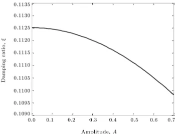
Using the analytical expressions obtained through Eqs. (25) and (28), one can investigate the inuence of system physical parameters on the frequency and damping ratio. For example, Figures 2 and 3 illustrate the variation of frequency and damping ratio with respect to the amplitude for the mentioned physical parameters, respectively. Further, by increasing the amplitude, the nonlinear frequency and damping ratio increase and decrease, respectively.
The investigations showed that for A > 1 and the same coecients as those mentioned before, the
Figure 1. The solutions obtained by Akbari-Ganji's Method (AGM) and numerical method for Example 1, A = 0:6.
Figure 2. The variation of frequency with respect to the initial amplitude for Example 1.
Figure 3. The variation of damping ratio with respect to the initial amplitude for Example 1.
obtained solution in Eq. (26) is of low accuracy. For instance, if the amplitude is selected as A = 1:5, the following solution will be obtained by AGM:
u(t) = 1:5077e 0:5tcos(4:92443t 0:10119): (29)
Figure 4 illustrates the above solution and indicates that it requires to be improved. In the current paper, the VIM is employed to improve AGM solution. For this problem, we have m = c = 1 and k = 20. After determining through Eq. (18), the Lagrange multiplier is obtained by Eq. (17) as follows:
() = sin(4:4441( t))
4:4441 e0:5( t): (30) By considering Eq. (29) as the zero-order solution (u0(t)) and substituting it into Eq. (13), the improved
solution (uIAGM) can be obtained through the following
Figure 4. The solutions obtained by Akbari-Ganji's Method (AGM), Improved AGM (IAGM), and numerical method for Example 1, A = 1:5.
uIAGM(t) = u0(t) + t
Z
0
sin(4:4441( t))
4:4441 e0:5( t)
u00
0() + u00() + u0() + u30() d: (31)
The solution and the phase plane diagrams of the current problem for A = 1:5 are illustrated in Figures 4 and 5, respectively. The improved solution obtained by Eq. (31) is in good agreement with the corresponding numerical solution. It should be noted that the phase plane diagram illustrates the oscillator displacement with respect to its velocity. For a conservative system, there is an equilibrium point in which the oscillator has a periodic motion around it. However, for a non-conservative system, the oscillation starts based on the assumed initial conditions and, then, the total
Figure 5. The phase plane diagram obtained by
Akbari-Ganji's Method (AGM), Improved AGM (IAGM), and numerical method for Example 1, A = 1:5.
energy of the system gradually decreases due to existing damping in the system. As can be seen, in the phase plane diagram (see Figure 5), the velocity of the system gradually decreases and, eventually, the oscillator comes to rest.
In the following, to investigate the eciency of AGM with respect to the non-zero initial velocity, the initial conditions are assumed as u(0) = 0:2 and _u(0) = 2. After solving Eq. (11) for the mentioned system parameters, the following solution is achieved:
u(t)= 0:46959e 0:50727tcos(4:46856t+1:130834):
(32) The above solution and its phase plane diagram are depicted in Figures 6 and 7, respectively. As can be seen, there is good agreement between the solution achieved by AGM and the numerical results. For the current problem and the same physical parameters, Nourazar and Mirzabeigy [18] obtained the following solution by the modied dierential transform method:
u(t) =e 2:0169t(0:00045 cos(12:6572t)
+ 0:0009614 sin(12:6572t)
+ e 0:4965t( 0:20045 cos(4:4826t)
+ 0:4239 sin(4:4826t)): (33) The comparison of the two solutions achieved through Eqs. (32) and (33) indicates that AGM solution is more concise.
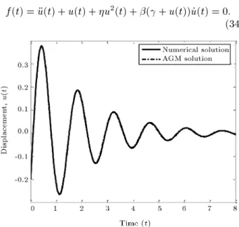
Example 2. Consider the dierential equation of a quadratic nonlinear damped oscillator as follows:
f(t) = u(t) + u(t) + u2(t) + ( + u(t)) _u(t) = 0:
(34)
Figure 6. The solutions obtained by Akbari-Ganji's Method (AGM) and numerical method for Example 1, A = 0:2, _u(0) = 2.
Figure 7. The phase plane diagram obtained by
Akbari-Ganji's Method (AGM) and numerical method for Example 1, A = 0:2, _u(0) = 2.
Eq. (34) that can present a kinetic model of abrin binding in an Epstein-Barr virus-transformed lympho-cyte culture [36] is solved by AGM. In this example, a non-zero value is supposed for the initial velocity. Therefore, the initial conditions are characterized by u(0) = A, _u(0) = B. Considering Eq. (10) as the trial solution of Eq. (34) and regarding the two steps given in Section 2, we have:
u(0) = A ! b cos ' = A; (35) _u(0) = B ! ab cos ' + !b sin ' = B; (36) f(0) !a2b cos ' + 2ab! sin ' !2b cos '
+b cos '+(+b cos ')( ab cos ' b! sin ') + b2cos2' = 0; (37)
f0(0) ! a3b cos ' 3a2b! sin ' + 3a!2b cos '
+ b!3sin ' ab cos ' b! sin '
2b2a cos2' 2!b2cos ' sin '
+ ( ab cos ' b! sin ')2+ ( + b cos ')
(a2b cos ' + 2ab! sin ' b!2cos ') = 0: (38)
Considering the physical values of Eq. (34) as A = 0:1, B = 0:05, = 1:1, = 0:7, and = 1:2, the solution to Eq. (34) is determined as follows:
u(t) = 0:1411e 0:4569tcos(0:961425t 0:78304): (39)
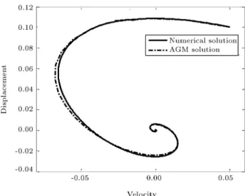
The solution and phase plane diagram obtained by AGM are illustrated in Figures 8 and 9, respectively.
Figure 8. The solutions obtained by Akbari-Ganji's Method (AGM) and numerical method for Example 2, A = 0:1, _u(0) = 0:05.
Figure 9. The phase plane diagram obtained by
Akbari-Ganji's Method (AGM) and numerical method for Example 2, A = 0:1, _u(0) = 0:05.
The comparison of AGM and numerical method reveals the high accuracy of AGM solution. Considering the current problem with such parameters as A = 0:5, B = 0, = 1, = 0:54, and = 1:435, AGM produces the following solution:
u(t) = 0:6305e 0:7462tcos(0:9712t 0:6551): (40)
As is depicted in Figure 10, the above solution has low accuracy. Similar to Example 1, the solution obtained by AGM is improved by the VIM. For the current problem, the Lagrange multiplier is as follows:
() = sin(0:9219(0:9219 t))e0:3875( t): (41)
Considering Eq. (40) as the zero-order solution (u0(t))
Figure 10. The solutions obtained by Akbari-Ganji's Method (AGM), Improved AGM (IAGM), and numerical method for Example 2, A = 0:5, _u(0) = 0.
Figure 11. The phase plane diagram obtained by Akbari-Ganji's Method (AGM), Improved AGM (IAGM), and numerical method for Example 2, A = 0:5, _u(0) = 0.
(uIAGM) can be obtained from the following correction
functional:
uIAGM(t)=u0(t) + t
Z
0
sin(0:9219( t))
0:9219 e0:3875( t)
u00
0()+(+u0())u00()+u0()+u20() d:
(42) Figures 10 and 11, which show the comparison between the achieved solutions and the numerical method, reveal that the solution of AGM can be easily improved by the VIM.
Example 3. For the last example, the transversal vibration of a exible beam with simply supported ends subjected to a constant axial load is considered. The
governed nonlinear dierential equation including non-linear terms in the damping coecient is as follows [4]:
f(t) =u(t) + ( u2(t) + u4(t)) _u + 2u(t)
u3(t) "u5(t) = 0: (43)
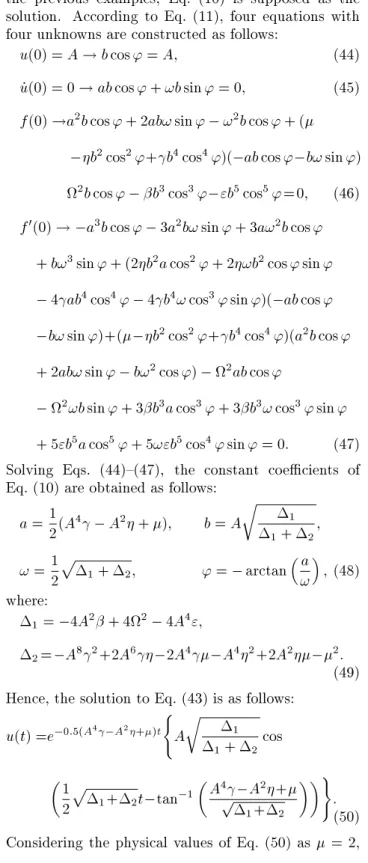
The initial conditions are supposed as u(0) = A, _u(0) = 0. To solve Eq. (43) via AGM, similar to the previous examples, Eq. (10) is supposed as the solution. According to Eq. (11), four equations with four unknowns are constructed as follows:
u(0) = A ! b cos ' = A; (44) _u(0) = 0 ! ab cos ' + !b sin ' = 0; (45) f(0) !a2b cos ' + 2ab! sin ' !2b cos ' + (
b2cos2'+b4cos4')( ab cos ' b! sin ')
2b cos ' b3cos3' "b5cos5'=0; (46)
f0(0) ! a3b cos ' 3a2b! sin ' + 3a!2b cos '
+ b!3sin ' + (2b2a cos2' + 2!b2cos ' sin '
4ab4cos4' 4b4! cos3' sin ')( ab cos '
b! sin ')+( b2cos2'+b4cos4')(a2b cos '
+ 2ab! sin ' b!2cos ') 2ab cos '
2!b sin ' + 3b3a cos3' + 3b3! cos3' sin '
+ 5"b5a cos5' + 5!"b5cos4' sin ' = 0: (47)
Solving Eqs. (44){(47), the constant coecients of Eq. (10) are obtained as follows:
a =1
2(A4 A2 + ); b = A r
1
1+ 2;
! =12p1+ 2; ' = arctan a!
; (48) where:
1= 4A2 + 42 4A4";
2= A82+2A6 2A4 A42+2A2 2:
(49) Hence, the solution to Eq. (43) is as follows:
u(t) =e 0:5(A4 A2+)t
( A
r 1
1+ 2cos
1 2
p
1+2t tan 1
A4 A2+
p
1+2
) : (50) Considering the physical values of Eq. (50) as = 2,
= 1:5, = 2:5, = 8, = 3:5, and " = 2, the displacement and phase plane diagrams for A = 0:5 are depicted and compared by numerical solution in Figures 12 and 13, respectively. Good agreement between the two methods can be seen. According to Eq. (27), the damping ratio () for the current problem can be found as follows:
= A4p A2 +
1+ 2 ; (51)
where 1 and 2 are given in Eq. (49). Eqs. (48)
and (51) can be utilized for studying the inuence of system physical parameters on the frequency and damping ratio. For example, the variation of frequency and damping ratio with respect to the amplitude for the mentioned physical parameters under dierent values of are illustrated in Figures 14 and 15, respectively.
Figure 12. The solutions obtained by Akbari-Ganji's Method (AGM) and numerical method for Example 3, A = 0:5.
Figure 13. The phase plane diagram obtained by Akbari-Ganji's Method (AGM) and numerical method for Example 3, A = 0:5.
Figure 14 reveals that, by increasing the amplitude, the nonlinear frequency decreases. In addition, for a specic value of amplitude, increasing results in a smaller frequency. Regarding Figure 15, it can be seen that, by increasing the amplitude, damping ratio decreases rstly and, then, increases. Moreover, for a specic value of the amplitude, by increasing , the damping ratio increases.
The investigations showed that, for A > 0:8, the obtained solution in Eq. (50) has low accuracy. For instance, if the amplitude is selected as A = 1, the following solution will be obtained by AGM:
u(t) = 1:02e 1:5tcos(7:5t 0:1974): (52)
The above solution, which is compared with the nu-merical solution in Figure 16, has low accuracy and, consequently, it should be improved in the same man-ner as the previous examples. According to Eq. (17),
Figure 14. The variation of frequency with respect to the initial amplitude for Example 3.
Figure 15. The variation of damping ratio with respect to the initial amplitude for Example 3.
the Lagrange multiplier is obtained as follows:
() = sin(7:9373(7:9373 t))e( t): (53)
Considering Eq. (52) as the zero-order solution (u0(t))
and substituting it into Eq. (13), the improved solution (uIAGM) can be obtained through the following
correc-tion funccorrec-tional:
uIAGM(t)=u0(t)+ t
Z
0
sin(7:9373( t)) 7:9373 e( t)
u00
0()
+ ( u2
0() + u40())u00()
+ 2u
0() u30() "u50() d: (54)
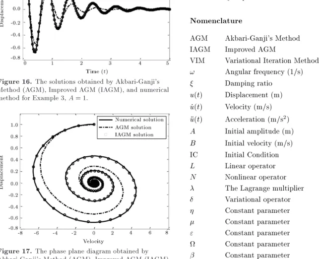
As is clear in Figures 16 and 17, AGM improved solu-tion (uIAGM) is in good agreement with the numerical
results.
Figure 16. The solutions obtained by Akbari-Ganji's Method (AGM), Improved AGM (IAGM), and numerical method for Example 3, A = 1.
Figure 17. The phase plane diagram obtained by Akbari-Ganji's Method (AGM), Improved AGM (IAGM), and numerical method for Example 3, A = 1.
5. Conclusion
In this paper, Akbari-Ganji's Method (AGM) was employed for solving three damped oscillatory systems with linear and nonlinear terms in damping coecients. Considering a simple trial solution for the correspond-ing dierential equation and, then, by applycorrespond-ing the initial conditions to the supposed answer, the main dierential equation, and its derivatives, the constant coecients of trial solution can be determined. AGM is a very simple procedure, because it can be easily implemented and does not need to introduce a new independent variable, which is common in some ana-lytical techniques such as harmonic balance method. Although AGM produces accurate solutions, in some problems, lower accuracy is achieved. In such cases, in contrast to the previously published papers proposed by a trial solution with higher-order terms, it was suggested that the solution obtained by AGM could be improved through the variational iteration method. The comparison of the results and those obtained by the numerical method conrmed the correctness and usefulness of the approach. Hence, AGM can be extended to other strong nonlinear problems with or without damping terms and, if necessary, its accuracy can be easily improved.
Nomenclature
AGM Akbari-Ganji's Method IAGM Improved AGM
VIM Variational Iteration Method ! Angular frequency (1/s) Damping ratio
u(t) Displacement (m) _u(t) Velocity (m/s) u(t) Acceleration (m/s2)
A Initial amplitude (m) B Initial velocity (m/s) IC Initial Condition L Linear operator N Nonlinear operator The Lagrange multiplier Variational operator Constant parameter Constant parameter " Constant parameter Constant parameter Constant parameter Constant parameter
References
1. Afsharfard, A. and Farshidianfar, A. \Design of nonlin-ear impact dampers based on acoustic and damping be-havior", International Journal of Mechanical Sciences, 65(1), pp. 125{133 (2012).
2. Leung, A.Y.T., Guo, Z., and Yang, H.X. \Residue harmonic balance analysis for the damped Dung resonator driven by a van der Pol oscillator", Inter-national Journal of Mechanical Sciences, 63(1), pp. 59{65 (2012).
3. Mansoori Kermani, M. and Dehestani, M. \Solving the nonlinear equations for one-dimensional nano-sized model including Rydberg and Varshni potentials and Casimir force using the decomposition method", Applied Mathematical Modelling, 37(5), pp. 3399{3406 (2013).
4. Zhang, W., Wang, F.-X., and Zu, J.W. \Local bifur-cations and codimension-3 degenerate bifurbifur-cations of a quintic nonlinear beam under parametric excitation", Chaos, Solitons & Fractals, 24(4), pp. 977{998 (2005).
5. Mohammadian, M. and Shariati, M. \Approximate analytical solutions to a conservative oscillator using global residue harmonic balance method", Chinese Journal of Physics, 55(1), pp. 47{58 (2017).
6. Mohammadian, M. and Akbarzade, M. \Higher-order approximate analytical solutions to nonlinear oscilla-tory systems arising in engineering problems", Archive of Applied Mechanics, 87(8), pp. 1317{1332 (2017).
7. Mohammadian, M. \Application of the global residue harmonic balance method for obtaining higher-order approximate solutions of a conservative system", Inter-national Journal of Applied and Computational Math-ematics, 3(3), pp. 2519{2532 (2017).
8. Mohammadian, M., Pourmehran, O., and Ju, P. \An iterative approach to obtaining the nonlinear frequency of a conservative oscillator with strong nonlinearities", International Applied Mechanics, 54(4), pp. 470{479 (2018).
9. Ganji, S.S., Ganji, D.D., Davodi, A.G., and Karim-pour, S. \Analytical solution to nonlinear oscillation system of the motion of a rigid rod rocking back using max-min approach", Applied Mathematical Modelling, 34(9), pp. 2676{2684 (2010).
10. Yazdi, M.K., Ahmadian, H., Mirzabeigy, A., and Yildirim, A. \Dynamic analysis of vibrating systems with nonlinearities", Communications in Theoretical Physics, 57(2), pp. 183{187 (2012).
11. De Rosa, M.A. and Lippiello, M. \Nonlocal Timo-shenko frequency analysis of single-walled carbon nan-otube with attached mass: An alternative Hamiltonian approach", Composites Part B: Engineering, 111, pp. 409{418 (2017).
12. Yazdi, M.K., Mirzabeigy, A., and Abdollahi, H. \Non-linear oscillators with non-polynomial and discontinu-ous elastic restoring forces", Nonlinear Science Letters A, 3(1), pp. 48{53 (2012).
13. Baltanas, J.P., Trueba, J.L., and Sanjuan, M.A.F. \Energy dissipation in a nonlinearly damped Dung oscillator", Physica D: Nonlinear Phenomena, 159(1{ 2), pp. 22{34 (2001).
14. Liao, S.-J. \An analytic approximate technique for free oscillations of positively damped systems with algebraically decaying amplitude", International Jour-nal of Non-Linear Mechanics, 38(8), pp. 1173{1183 (2003).
15. Cveticanin, L. \Oscillators with nonlinear elastic and damping forces", Computers & Mathematics with Ap-plications, 62(4), pp. 1745{1757 (2011).
16. Shamsul Alam, M., Roy, K.C., Rahman, M.S., and Mossaraf Hossain, M. \An analytical technique to nd approximate solutions of nonlinear damped oscillatory systems", Journal of the Franklin Institute, 348(5), pp. 899{916 (2011).
17. Wu, B.S. and Sun, W.P. \Construction of approximate analytical solutions to strongly nonlinear damped os-cillators", Archive of Applied Mechanics, 81(8), pp. 1017{1030 (2011).
18. Nourazar, S. and Mirzabeigy, A. \Approximate solu-tion for nonlinear Dung oscillator with damping ef-fect using the modied dierential transform method", Scientia Iranica, 20(2), pp. 364{368 (2013).
19. Cveticanin, L. \On the truly nonlinear oscillator with positive and negative damping", Applied Mathematics and Computation, 243, pp. 433{445 (2014).
20. Ene, R.D., Marinca, V., and Marinca, B. \Free oscilla-tions of a nonlinear oscillator with an exponential non-viscous damping", Applied Mechanics and Materials, 801, pp. 38{42 (2015).
21. Herisanu, N. and Marinca, V. \An optimal homotopy asymptotic approach to a damped dynamical system of a rotating electrical machine", Applied Mechanics and Materials, 801, pp. 202{206 (2015).
22. Razzak, M.A. and Molla, M.H.U. \A new analyti-cal technique for strongly nonlinear damped forced systems", Ain Shams Engineering Journal, 6(4), pp. 1225{1232 (2015).
23. Sheikholeslami, M. and Ganji, D.D. \Nanouid ow and heat transfer between parallel plates considering Brownian motion using DTM", Computer Methods in Applied Mechanics and Engineering, 283, pp. 651{663 (2015).
24. Mohammadian, M., Hosseini, S.M., and Abolbashari, M.H. \Lateral vibrations of embedded hetero-junction carbon nanotubes based on the nonlocal strain gradi-ent theory: Analytical and diergradi-ential quadrature el-ement (DQE) methods", Physica E: Low-dimensional Systems and Nanostructures, 105, pp. 68{82 (2018).
25. Sheikholeslami, M. and Ganji, D.D. \Magnetohy-drodynamic ow in a permeable channel lled with nanouid", Scientia Iranica, B, 21(1), pp. 203{212 (2014).
26. Ebaid, A., Rach, R., and El-Zahar, E. \A new analyti-cal solution of the hyperbolic Kepler equation using the Adomian decomposition method", Acta Astronautica, 138, pp. 1{9 (2017).
27. Pakdemirli, M. \Perturbation-iteration method for strongly nonlinear vibrations", Journal of Vibration and Control, 23(6), pp. 959{969 (2017).
28. Akbari, M.R., Ganji, D.D., Majidian, A., and Ahmadi, A.R. \Solving nonlinear dierential equations of Van-derpol, Rayleigh and Dung by AGM", Frontiers of Mechanical Engineering, 9(2), pp. 177{190 (2014).
29. Mirgolbabaee, H., Ledari, S.T., and Ganji, D.D. \New approach method for solving Dung-type nonlinear oscillator", Alexandria Engineering Journal, 55(2), pp. 1695{1702 (2016).
30. Akbari, M.R., Ganji, D.D., Nimafar, M., and Ahmadi, A.R. \Signicant progress in solution of nonlinear equations at displacement of structure and heat trans-fer extended surface by new AGM approach", Frontiers of Mechanical Engineering, 9(4), pp. 390{401 (2014).
31. Akbari, M.R., Ganji, D.D., Rostami, A.K., and Nima-far, M. \Solving nonlinear dierential equation gov-erning on the rigid beams on viscoelastic foundation by AGM", Journal of Marine Science and Application, 14(1), pp. 30{38 (2015).
32. Mirgolbabaee, H., Ledari, S.T., and Ganji, D.D. \An assessment of a semi analytical AG method for solving nonlinear oscillators", New Trends in Mathematical Sciences, 4(1), pp. 283{299 (2016).
33. He, J. \A new approach to nonlinear partial dierential equations", Communications in Nonlinear Science and Numerical Simulation, 2(4), pp. 230{235 (1997).
34. Daeichi, M. and Ahmadian, M. \Application of varia-tional iteration method to large vibration analysis of slenderness beams considering mid-plane stretching", Scientia Iranica. Transactions B, Mechanical Engi-neering, 22(5), pp. 1911{1917 (2015).
35. Mohammadian, M. \Application of the variational iteration method to nonlinear vibrations of nanobeams induced by the van der Waals force under dierent boundary conditions", The European Physical Journal Plus, 132(4), p. 169 (2017).
36. Witten, M. and Siegel, D. \A kinetics model of abrin binding in a virus transformed lymphocyte cell culture", Bulletin of Mathematical Biology, 44(4), pp. 453{476 (1982).
Biographies
Mostafa Mohammadian received his BSc degree in Mechanical Engineering from Ferdowsi University of Mashhad, Iran in 2007 and the MSc degree in applied Mechanical Engineering from Semnan Univer-sity, Semnan, Iran in 2009. Also, he received his PhD degree in Mechanical Engineering from Ferdowsi University of Mashhad, Iran in 2019. Moreover, he is a faculty member and the Head of the Department of Mechanical Engineering in Islamic Azad University, Gorgan branch, Kordkuy center, Iran. His research interests include nonlinear dynamics and vibration, numerical methods, optimization and approximate an-alytical methods.
Mahmoud Shariati is a Full Professor in Ferdowsi University of Mashhad, Iran. He was educated in the mechanical engineering eld and, now, is teaching at the Department of Mechanical Engineering in Ferdowsi University of Mashhad, Iran. His research focuses on the nonlinear dynamics, fracture mechanics and fatigue, stress analysis, design of mechanical structures, and nano-mechanics. He has published more than 250 scientic papers and books.