The effects of stress and sex on selection, genetic covariance,
and the evolutionary response
L . H O L M A N * & F . J A C O M B†
*School of BioSciences, University of Melbourne, Parkville, VIC, Australia
†Research School of Biology, Australian National University, Canberra, ACT, Australia
Keywords: B matrix;
environmental stress; fitness landscape; G matrix; Robertson–Price.
Abstract
The capacity of a population to adapt to selection (evolvability) depends on whether the structure of genetic variation permits the evolution of fitter trait combinations. Selection, genetic variance and genetic covariance can change under environmental stress, and males and females are not geneti-cally independent, yet the combined effects of stress and dioecy on evolv-ability are not well understood. Here, we estimate selection, genetic (co)variance and evolvability in both sexes ofTribolium castaneumflour bee-tles under stressful and benign conditions, using a half-sib breeding design. Although stress uncovered substantial latent heritability, stress also affected genetic covariance, such that evolvability remained low under stress. Sexual selection on males and natural selection on females favoured a similar phe-notype, and there was positive intersex genetic covariance. Consequently, sexual selection on males augmented adaptation in females, and intralocus sexual conflict was weak or absent. This study highlights that increased heri-tability does not necessarily increase evolvability, suggests that selection can deplete genetic variance for multivariate trait combinations with strong effects on fitness, and tests the recent hypothesis that sexual conflict is weaker in stressful or novel environments.
Introduction
Evolvability refers to the capacity of a population to undergo adaptation. Identifying the main factors responsible for variation in evolvability is a key chal-lenge for biologists, with ramifications for conservation biology and selective breeding. Firstly, the structure of genetic variance and covariance in the population is a key predictor of evolvability. Genetic variance is essen-tial for evolution, and genetic covariance among differ-ent traits can hamper adaptation by constraining their independent evolution. However, genetic covariance can also accelerate adaptation if it happens to align with the trait combination under selection, by allowing adaptation in one trait to augment adaptation in another (Blows & Hoffmann, 2005; Agrawal & Stinch-combe, 2009; Walsh & Blows, 2009).
Secondly, genetic (co)variance sometimes changes when measured in different environments (reviewed in Wood & Brodie, 2015), meaning that the environment (abiotic or biotic) might be another important predictor of evolvability. In particular, stressful environments have been proposed to either increase or decrease genetic variance (reviewed in Hoffmann & Meril€a, 1999), and to change the strength of selection (Agrawal & Whitlock, 2010). Presently there is no empirical con-sensus about the effect of stress on evolvability (Char-mantier & Garant, 2005; Wood & Brodie, 2015).
Genetic covariance between the sexes represents a third factor influencing evolvability. For example, ‘in-tralocus sexual conflict’ is the concept that some traits have sex-specific optimal values, but the evolu-tion of adaptive sexual dimorphism is constrained by intersex genetic covariance, leading to a maladaptive phenotypic compromise (e.g. Lande, 1980; Bondurian-sky & Chenoweth, 2009; Lewis et al., 2011; Gosden
et al., 2012; Stearns et al., 2012; Wyman et al., 2013;
Berger et al., 2014a; Ingleby et al., 2014). Literature reviews suggest that genetic covariance between male
Correspondence:Luke Holman, School of BioSciences, University of
Melbourne, Parkville, VIC 3010, Australia.
and female traits is often strong and positive (Poissant
et al., 2010) and that roughly 20% of traits that have
been the subject of two-sex selection analyses are under sexually antagonistic selection (Morrissey, 2016), implying that intralocus sexual conflict is com-mon. Additionally, some studies have found that measures of male and female fitness are negatively genetically correlated (e.g. Chippindale et al., 2001; Fedorka & Mousseau, 2004; Delcourt et al., 2009; Poissant et al., 2010; Berger et al., 2014a), which implies that the majority of genetic variance in fitness is sexually antagonistic. However, genetic links between the sexes can also increase evolvability. For example, if both sexes are selected for large body size, female body size (and therefore fitness) will evolve upwards more rapidly when there is positive intersex genetic covariance for body size (e.g. Lande, 1980; Agrawal & Stinchcombe, 2009; Wyman et al., 2013). In theory, selection on males can even increase evolvability enough to counteract the ‘two-fold cost of sex’, explaining the predominance of sex-ual reproduction over asexsex-uality (e.g. Agrawal, 2001; Siller, 2001).
Recently, researchers have begun to consider the effects of stress and sex on genetic (co)variance simulta-neously, and to examine how they interact to affect evolvability. Theoretical models (e.g. Lande, 1980; Con-nallon, 2015; Connallon & Hall, 2016) predict that intralocus sexual conflict should be stronger in environ-ments to which the population is well adapted, because persistent selection depletes variation at loci with sexu-ally concordant fitness effects, elevating the relative importance of sexually antagonistic genetic variation. Accordingly, some empirical studies have found that the intersex genetic correlation for fitness becomes more positive in comparatively stressful environments (e.g. Long et al., 2012; Berger et al., 2014b; Punzalan
et al., 2014). However, not all results have supported
this prediction (Delcourt et al., 2009; MacLellan et al., 2012), and much remains unknown. For example, there are insufficient data to determine whether male and female traits become more or less genetically corre-lated under stress, if sex differences in selection change under stress, or how the combination of these factors affects evolvability.
Here, using a multivariate quantitative genetic approach (e.g. Steven et al., 2007; Lewis et al., 2011; Gosdenet al., 2012; Stearns et al., 2012; Reddiexet al., 2013; Wymanet al., 2013; Berger et al., 2014b;
Punza-lan et al., 2014; Walling et al., 2014), we investigate
selection and genetic (co)variance in both sexes, across both stressful and benign conditions, inTribolium casta-neumflour beetles. We test for sex differences in selec-tion, describe how stress alters genetic (co)variance within and between sexes and finally combine these data to ascertain how stress, sex and their interaction affect evolvability.
Materials and methods
Beetle culturing
We used a population of T. castaneumin long-term lab-oratory culture, named QTC4 (Collins, 1998). The QTC4 culture was maintained at a population size ofc. 400 breeding adults in 1-L glass jars filled with 700 g 20 : 1 organic wholemeal flour and yeast (progeny are mixed across jars each generation). Virgins were obtained by collecting and sexing pupae from the stocks and allowing them to mature in single-sex Petri dishes filled with yeasted flour. Beetles were kept in a climate room at 29 °C on a 12 : 12-h photocycle. T. castaneum
is a promiscuous species in which both sexes can mate several times per day, and has last-male sperm prece-dence (Michalczyk et al., 2010). Thus, we hypothesize that fitness differences between adult males are largely determined by scramble competition for access to females and their gametes, whereas female fitness hinges on laying many viable eggs. We are not aware of any direct measurements of intralocus sexual conflict in this species, although males and females differ phe-notypically (this study), which implies that sex-specific selection is present, or was present in the past (Bon-duriansky & Chenoweth, 2009).
Breeding design and trait measurements
We conducted a split-brood paternal half-sib breeding design, in which 36 ‘sires’ were mated to three ‘dams’ each. The eggs from each dam were divided evenly between two dietary treatments, termed ‘high food’ and ‘low food’. All sires and dams were 10–11 days old post-eclosion. We aimed to measure four variables (ely-tra length, body mass and development time – chosen due to their likely selective importance – as well as male- and female-specific metrics of fitness) in four sons and four daughters per dam. Occasionally, we were unable to measure eight offspring per dam, or to measure all four variables on a given offspring. In total, we obtained complete measurements of 1301 offspring and incomplete measurements of 1355 offspring (or
n =3576, if counting offspring for which we only mea-sured development time; see below), from 36 sires and 104 dams. Incomplete measurements occurred in a ran-dom fashion when beetles were lost or damaged.
The low food diet contained a 4 : 1 ratio of micro-crystalline cellulose to flour; the cellulose has a similar particle size to flour and served as a nutritive, non-toxic ‘filler’. Previous experiments demonstrated that larvae developing in flour containing higher propor-tions of cellulose develop more slowly and eclose into adults that are comparatively light for their size (Lewis
et al., 2012), illustrating that the low food treatment is
‘stressful’. The high food diet contained a 1 : 4 ratio of filler to flour.
Pairs of beetles were mated by placing them on filter paper under a 35-mm Petri dish. After copulating, dams were moved to a 50-mL Petri dish filled with 4 g of diet; the type of diet was alternated such that every other female was placed in low food diet. After 24 h, dams were moved into a new Petri dish containing 4 g of the other type of diet. The dams were moved to new dishes four more times every 24 h, alternating the type of diet in the new Petri dish each time. Therefore, all dams were given 24 h to lay eggs in six different Petri dishes, three for each diet treatment. Females were removed from their final Petri dish after 24 h. This pro-cedure ensured that larval density was low for all females (median: 11 adults eclosing per dish), that the order of mating and laying was balanced across food treatments and that the laying date of all progeny was known to the nearest 24 h. To minimize the number of dams that failed to lay eggs due to incomplete sperm transfer, the sires were housed with one of their dams throughout the egg laying period. Every 12 h, the sires were transferred to a dish holding one of their other dams, ensuring that the amount of male contact was equal for all dams. The Petri dishes were moved daily around the climate room, preventing any microclimatic differences from systematically influencing any particu-lar dish.
The Petri dishes were scanned daily for pupae, which were removed and sexed, and placed in individual gel capsules with a pinch of flour–yeast mixture. The pupae were checked daily to record the date of eclosion into adults. We thus determined egg-to-adult develop-ment time to the nearest day for all progeny from every dam. We selected four sons and four daughters per dam using a random number generator and collected additional trait data (besides development time) on them.
We assayed the fitness of 9-day-old female offspring by placing them in a Petri dish containing 4 g 1 : 1 flour and cellulose, along with two 9- to 15-day-old virgin males from the stocks. All three beetles were removed after 5 days, and we later counted the num-ber of adult progeny that emerged as a proxy for female fitness.
Nine days after eclosion, male beetles were placed in a 55-mm Petri dish with two randomly chosen virgin females (aged 9–15 days) for 1 h. The two females were then placed in gel capsules filled with flour and kept for a month before being frozen. We then inspected the contents of the capsules for developing offspring, which indicated whether the focal male had successfully inseminated each female. We used the number of females inseminated (0, 1 or 2) as a proxy for male fit-ness (thus, we assume that males that can rapidly find and mate with females would sire more offspring over their lives).
Males and females were freeze-killed immediately after completion of their fitness assays. We later
recorded their dry mass to the nearest 0.01 mg using a Mettler Toledo XS105DU balance and then measured the length of the elytra to the nearest 0.02 mm using a microscope eyepiece graticule. Trait measurements were blind to food treatment, sex and parentage.
Statistical analysis
Measuring sex-specific selection
We performed a multivariate selection analysis follow-ing Lande & Arnold (1983). We first calculated relative fitness, by dividing each individual’s absolute fitness by mean absolute fitness (calculated from members of the same sex from the same food treatment). For each combination of sex and food treatment, we fitted a regression with relative fitness as the dependent vari-able and the three phenotypic traits as linear predictors, each of which was scaled to have a mean of zero and standard deviation of one. The three slope estimates for males and females provided our estimates of the vectors of sex-specific standardized directional selection gradi-ents, termed bm and bf, respectively, for both of the food treatments.
We then fitted two more regressions (one for each sex) using the same three linear predictors, as well as the three quadratic terms and the three cross-product terms. After doubling our quadratic regression coeffi-cients (Stinchcombe et al., 2008), we obtained our esti-mates of all elements ofcm and cf, that is the matrices of quadratic and correlational selection gradients for males and females.
As relative fitness was non-normal, we used permu-tation tests (rather than P-values from regression) to test which elements of b and c differed significantly from zero. The test involved randomly permuting rela-tive fitness among same-sex individuals, recalculating
bm,bf,cm andcf, repeating 105times, then comparing the observed values with the null distribution to obtain two-tailedP-values.
Comparing multivariate selection between sexes and environments
We tested whether sex and food treatment affected the strength and form of directional and nonlinear selection on the three phenotypic traits using an approach inspired by Chenoweth & Blows (2005), but using AIC model selection (Anderson, 2007) instead of multiple
F-tests.
Specifically, we began by listing the set of models we wished to compare (Anderson, 2007). For directional selection, the simplest model in the set contained sex, food and the three phenotypic traits as predictors, which represents the hypothesis that selection is nei-ther sex- nor treatment-specific. The onei-ther models addi-tionally contained all three food-by-trait interactions, all three sex-by-trait interactions or both set of interac-tions, representing the hypotheses that selection is
affected by sex, food treatment or both. The most com-plex model additionally contained the food-by-sex-by-trait interactions, which represents the hypothesis that selection is sex-specific in a manner that depends on food treatment.
We used a similar approach to investigate whether food and sex affected nonlinear selection; here, the model set began with the most complex model from the previous exercise, plus the three quadratic terms for the three traits. The more complex models added inter-actions between food and sex to the quadratic terms.
Finally, we also calculated the angle, in degrees, between bm and bf as cos1 b
mbf=
ffiffiffiffiffiffiffi b2
m
q ffiffiffiffiffi b2 f
q
180=p, where large angles indicate that males and females are selected for different trait combinations. To test whether these two angles were significantly greater than expected under the null hypothesis that selection is not sex-specific, we used a permutation test in which the sex of each individual was randomly shuffled, and the angle was recalculated. We calculated the one-tailed
P-value as the proportion of 10 000 permutations in which the angle was larger than expected. We also tested whether the angle differed between high and low food treatments, by randomly shuffling the food treatments across individuals to obtain the null distribution for the difference in angles, and comparing it to the observed difference.
Estimating additive genetic (co)variance for phenotypic traits
When traits are measured in two sexes, the additive genetic variance–covariance matrix (G) can be decom-posed as follows:
G¼ Gf B BT G
m
(1)
where Gf and Gm are the within-sex additive genetic
variance–covariance matrices for females and males, B describes the additive genetic covariance for each trait between the sexes and T denotes matrix transposition (Lande, 1980).
We estimated G for our six phenotypic traits (i.e. female and male elytra length, mass and development time) using Bayesian mixed models implemented in the MCMCGLMM package for R (Hadfield, 2010). The
trait values were first scaled to have a mean of zero and a standard deviation of one, and G was esti-mated as the posterior mode of the sire-level (co)vari-ances multiplied by four (as half-sibs share, on average, a quarter of their alleles through common descent). Thus, the genetic variances presented in Table 2 are equivalent to narrow-sense heritability, h2
(i.e. the proportion of phenotypic variance attributa-ble to additive genetic effects). For all MCMCglmm
models in this study, we assumed a Gaussian distribu-tion for all traits and used parameter-expanded priors with prior means set to zero and a diagonal prior covariance matrix with variances set to 1000 (multi-ple alternative priors were tested, and gave very simi-lar results throughout). As individuals cannot be both sexes, residual covariance was estimated among male traits and among female traits, but not between male and female traits. All models were run for 500 000 iterations with a thinning interval of 450 and a burn-in of 50 000. We ran models multiple times to verify convergence and checked for autocorrelation in the chains.
First, to measure and compare G in high and low food conditions, we estimated G using two separate models, which each used individuals from a single treatment. These model fit Sire, Dam and Dish as ran-dom intercepts. Thus, we estimated the degree of simi-larity among individuals that shared the same father after controlling for similarity among individuals that shared the same mother, or were raised in the same Petri dish.
To test for genotype-by-environment interactions (G9E) for our six phenotypic traits, we fit another MCMCglmm model that used all of data (i.e. high and low food individuals). As well as containing the random effects Sire, Dam and Dish, this model additionally con-tained a sire9food random regression slope. If the effect of some genotypes on the phenotype differs between food treatments, we expect some of the ran-dom slope effects to differ from zero.
Estimating additive genetic (co)variance for male and female fitness components
As before, we first split the data by food treatment and fit an MCMCglmm model of male relative fitness and female relative fitness (both scaled to mean 0 and vari-ance 1) with the random effects Sire, Dam and Dish. This allowed measurement of the heritability of fitness and the genetic covariance between them, under high and low food conditions. Additionally, we again fit a model of all the data (high and low food together) that additionally contained a sire9food random slope, to test for G 9E effects on fitness.
Estimating the response to selection
To quantify the ability of the population to respond to selection (i.e. evolvability), we calculated the response to selection using two complementary methods, namely the multivariate breeder’s equation (also called the Lande equation), and the Robertson–Price identity (also called the Secondary Theorem of Natural Selection). These two approaches are contrasted in Morrissey et al.
(2012) and Stinchcombe et al.(2014). Both approaches yield an estimate of, that is the vector of changes in population mean phenotype resulting from selection, measured in standard deviations.
Following Lande (1980), we estimated the evolution-ary response for a population in environmentjas
DZfj
DZmj
¼1 2Gj
bfj
bmj
(2) whereZij represents the predicted evolutionary change in the population mean trait values for sex i in envi-ronment j, Gj is the additive genetic variance–
covari-ance matrix (eqn 1) as measured in environmentjand thebterms are the corresponding vectors of sex-specific directional selection measured in environment j. The factor 1/2 appears because male and female parents are assumed to make equal genetic contributions to both sexes of offspring (i.e. we assume a negligible amount of sex-linked genetic variance for the focal traits).
To estimate the confidence limits on DZ, we calcu-lated eqn 2 using the 1000 samples of the posterior
dis-tribution of G from the appropriate MCMCglmm
model. To ensure that the confidence limits onDZalso incorporated uncertainty in our estimation of b, we generated 1000 estimates b values by bootstrap resam-pling of the data set and paired each one with a ran-domly chosen posterior estimate of G. The 95% quantiles on DZ were used as estimates of the 95% confidence limits.
The Robertson–Price identity states that the response to selection of a trait, z, is equivalent to the additive genetic covariance between that trait and relative fit-ness, denoted rA(w, z). We thus estimated rA(w, z) via 12 separate bivariate MCMCglmm models, one for each of the six traits and two food treatments. Each model used data from the focal environment only and had the scaled trait value and unscaled relative fitness as the response variables, and sire, dam and dish as random effects. We used the posterior mode and 95% credible intervals ofrA(w,z) to derive our estimate ofDZ. Testing for genetic variation in the trait combination under selection
We first estimated the amount of additive genetic vari-ance for the linear trait combination under directional selection, which we termzb, by projectingbonto theG matrix via the projection equation bTGb (Blows et al., 2004). We performed this analysis using estimates of b and G from the high and low food treatments. To obtain confidence limits on VA(zb), we used the 1000 posterior estimates ofGfrom the relevant MCMCglmm model and generated 1000 paired estimates of b by bootstrapping (just as for the breeder’s equation analy-sis; see above), giving the estimated distribution of VA(zb) values supported by the data. We then took the mode and 95% quantiles of this distribution.
We next measured the angle between the major axis of genetic variance (i.e. gmax, the leading
eigen-vector of G) and the vector of selection, providing a complementary measure of genetic variance for the selectively favoured trait combination. To obtain
confidence limits on this angle, we obtained the poste-rior distribution of gmax from the posterior of G,
generated 1000 paired estimates of b by bootstrapping (as in the previous analysis) and estimated the distribu-tion of angles supported by the data as cos1 bg
max= ð
ffiffiffiffiffi b2
p ffiffiffiffiffiffiffiffiffiffi
g2 max
p
Þ 180=p.
Identifying genetic covariances that constrain or augment adaptation
A key aim of this study is to test whether genetic covari-ance between the sexes assists or hinders adaptation, under both stressful and benign conditions. We there-fore calculated the magnitude of genetic constraints using two complementary metrics, namely R (Agrawal & Stinchcombe, 2009) andh(Walsh & Blows, 2009).
In short,R is the ratio between the increase in aver-age fitness due to adaptation that is predicted when entering the observed value of G into eqn 2, and the fitness increase that is predicted when entering a modi-fied version ofGin which some or all of the covariance terms have been set to zero. R<1 indicates that the focal set of covariances is constraining adaptation, whereasR >1 suggests it is augmenting adaptation. We calculated R after setting to zero: (a) the within-sex genetic covariance, (b) the between-sex genetic covari-ance or (c) both; this analysis reveals which compo-nents ofGassist or hinder adaptation.
By contrast,h is the angle between the evolutionary response vector and the vector of directional selection
b. A value of h=0 indicates that evolutionary change is proceeding in precisely the direction that maximizes the increase in fitness, whereas positivehsuggests that constraints in G are deflecting evolutionary change away from the optimal direction (Walsh & Blows, 2009). As before, we investigated the effects onhof set-ting the within-sex genetic covariance, the between-sex genetic covariance or both, to zero; this allows us to determine which components ofGare most responsible for deflecting the evolutionary response away from the direction that maximizes the increase in fitness.
We estimated the posterior distribution of R and h from the posterior distribution of G provided by the
MCMCglmmmodel, again paired with values ofb
gener-ated by bootstrap resampling of the data. This allowed calculation of 95% credible intervals for all estimates of
R and hthat incorporate uncertainty in our estimation of both Gand b, facilitating hypothesis testing. Appen-dix 1 gives a detailed explanation of the calculation of R andh.
Results
Sexual dimorphism, environmental effects and phenotypic correlations
Females were heavier than males (means SE:
beetles from the low food treatment were 7% lighter than those from the high treatment (1.330.010 mg, 1.240.010 mg). The effects of sex (t1336=9.70,
P<0.0001), food (t1336=6.58, P<0.0001) and the sex9diet interaction (t1336 =2.30, P =0.021) were significant in a linear model. The interaction indicated that the low food diet had a stronger effect on female mass than male mass.
Females had a slightly longer elytrum than males (2.530.004 mm and 2.500.004 mm; t1193=5.19,
P<0.0001), and elytrum length was 3% lower in bee-tles reared in low food conditions (2.55 0.004 mm and 2.480.004 mm; t1193=9.77, P<0.0001). There was no sex9diet interaction (t1193 =1.76,P =0.079).
Egg-to-adult development time was shorter in
females than males, but not significantly so
(37.84 0.06 and 37.920.06 days; t3572=1.95,
P=0.051), and was 4% longer in the low food
treat-ment (37.21 0.05 and 38.720.06 days;
t3572 =14.3, P<0.0001). There was no sex9food interaction (t3572=1.69,P =0.092).
Female fitness was elevated by 5% in the high food treatment (Poisson GLM: z648=2.02, P=0.043; 13.20.4 vs. 12.60.4 offspring). Male fitness was also elevated, but not significantly so (Mann–Whitney
U=59 605, n=675, P=0.21; 1.050.03 vs. 1.000.03 matings).
Phenotypic covariance among the three traits was mostly positive, except that fast-developing males tended to be slightly larger than slow-developing ones (Table S1). As expected, elytra size and body mass covaried, but there was nevertheless substantial varia-tion in mass among beetles of similar length (regres-sion: R2=0.24), justifying treating mass and elytra length as separate traits.
Sex differences in directional and nonlinear phenotypic selection
We performed phenotypic selection analyses on the subset of individuals for which fitness plus all three traits were successfully measured (n=1301). In both sexes and food treatments, there was positive direc-tional selection on body mass (Table 1). There was neg-ative directional selection on elytra length in females, whereas selection on male elytra length was either weaker or reversed, depending on food treatment. Selection on development time was negative (i.e. fast development was favoured), except in males raised on high food.
When comparing different models of fitness, the top model in our model set contained the three food-by-trait interactions and the three sex-by-food-by-trait interactions, illustrating that selection differed significantly between sexes and also between food treatments (Table S2; DAIC=4.94 relative to the next best-fitting model). Specifically, directional selection favoured a different
combination of elytra length and mass in each sex, and selection for faster development appeared stronger in females (Table 1). Additionally, directional selection was weaker in the low food treatment, and in some cases changed direction (Table 1). The model contain-ing the three food-by-sex-by-trait interaction terms was substantially worse than the model that lacked these terms (DAIC=7.81), indicating that the effect of sex on selection did not vary significantly across food treat-ments (or alternatively, that selection was not more environment-dependent in one sex than the other).
In the high food treatment, the angle betweenbfand
bmwas 25°(bootstrapped 95% CIs: 7°–53°), whereas in low food this angle was 62° (22°–125°); the change in angle was not significant (permutation test: one-tailed
P =0.053). Neither of these angles differed significantly from the distribution of angles predicted under the null hypothesis that selection is not sex-specific (permuta-tion test; one-tailed P=0.14 in high food andP=0.09 in low food).
The diagonal elements ofcmandcfwere mostly neg-ative, suggesting the operation of stabilizing selection in both sexes (Table 1). The exception was male elytra length, which was under nonsignificant disruptive selection in both food treatments. All three of the off-diagonal elements differed in sign between males and females, although these differences were small in mag-nitude. Moreover, most elements of cm and cf did not differ significantly from zero (permutation test; a=0.05); the exceptions were the negative quadratic effects of female mass in high food (P=0.021) and male development time in low food (P=0.024). AIC model selection suggested that nonlinear selection did not differ significantly between sexes or food treat-ments (Table S3).
Effects of diet and sex on genetic variance and covariance
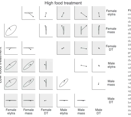
We first estimated G in the high and low food treat-ments, by splitting the data by food treatment and run-ning two separate MCMCglmm models (n =1994 and 1582 in high and low food, respectively). Figure 1 and Table 2 illustrate that all heritabilities and genetic covariances were close to zero in the high food treat-ment, except for female mass. By contrast, heritabilities were higher in the low food treatment, and some of the genetic covariances were significantly positive. Here, mass and elytra length were positively genetically correlated, and the intersex genetic correlations were of a similar magnitude to the within-sex correlations. Ely-tra length and body mass were more heritable than development time, and genetic (co)variance was slightly more positive in females than males. The addi-tive genetic correlations (not shown) were universally positive on low food, and their 95% CIs often excluded zero (Table S4). Under high food, genetic correlations
could not be measured accurately due to the low genetic variances.
The eigenvalue of the leading eigenvector of G (‘gmax’) was 4.6-fold larger when G was estimated in
the low food relative to high, reflecting the greater genetic variance in low food conditions. Moreover, gmax captured 98% of the variance in G in low food
(95% credible intervals estimated from the posterior of G: 75–99%) and 85% (54–98%) in high food. Thus, even though low food conditions elevated genetic vari-ance, the dimensionality ofGwas low in both environ-ments (Fig. 1), such that evolution was largely only possible along a single trait axis, namelygmax.
To test for G9E effects on our six phenotypic traits, we fit another model that used all the data, that is all individuals from both food treatments for which we had measured at least one trait (n=3576). There was considerable genetic (co)variance in the random slopes for male development time, female development time and their covariance, suggesting that some of the alleles underlying variance in development time have effects that depend on the presence/absence of food stress (Fig. S1).
Additive genetic (co)variance for fitness components
We found that in high food conditions, the narrow-sense heritability (h2) of female relative fitness was 0.004 (95% CIs: 0.000–0.58), whereas that of male mating success was 0.002 (0.000–0.30); the genetic covariance between them was 0.12 (0.78 to 0.92).
The situation was similar in the low food treatment:h2
was 0.003 (0.000–0.46) for females and 0.001 (0.000– 0.19) in males, and the genetic covariance was 0.79 (0.73 to 0.99).
Although these measures of genetic variance in fit-ness are imprecise, we had good statistical power to measure the alignment of genetic variance with selec-tion (via the projecselec-tion equaselec-tion bTGb). There was minimal genetic variance for the linear trait combina-tion under direccombina-tional seleccombina-tion, zb, in both the high food (VA(zb) =0.010, 95% CIs: 0.0008–0.051) and low food treatments (0.002, 0.0001–0.021). Additionally, the vector of directional selection b was misaligned with the major axis of genetic variance,gmax: the angle
betweenb andgmaxwas 61°(95% CIs: 36–85) in high
food and 70°(49–90) in low food.
Using random regression, we found that G9E for fitness was either absent or weak. The additive genetic variance in regression slopes was 0.0006 (0.000–0.16) for female fitness, 0.0004 (0.000–0.11) for male fitness and 0.0002 for their genetic covariance (0.027 to 0.053).
Magnitude of the response to selection
The estimated change in mean phenotype in response to selection was on the order of 0–0.02 standard devia-tions when measured with the multivariate breeder’s equation, and even closer to zero when using the Robertson–Price identity (Table S5). The fact that the breeder’s equation produced larger estimates of than did the Robertson–Price identity might indicate the
Table 1 The vector of directional phenotypic selection gradients,b, and the matrix of nonlinear phenotypic selection gradients,c, for each
sex, as measured in the high food and low food treatments.
b
c
Elytra length Body mass DT
Females (high)
Elytra length 0.141 (0.034) 0.049 (0.053) 0.018 (0.045) 0.030 (0.039)
Body mass 0.170 (0.035) 0.116 (0.048) 0.022 (0.041)
DT 0.034 (0.032) 0.080 (0.049)
Males (high)
Elytra length 0.068 (0.036) 0.003 (0.051) 0.029 (0.040) 0.046 (0.044)
Body mass 0.191 (0.036) 0.046 (0.051) 0.066 (0.041)
DT 0.021 (0.036) 0.063 (0.064)
Females (low)
Elytra length 0.068 (0.040) 0.038 (0.060) 0.003 (0.049) 0.044 (0.050)
Body mass 0.084 (0.038) 0.058 (0.063) 0.039 (0.039)
DT 0.063 (0.034) 0.005 (0.038)
Males (low)
Elytra length 0.035 (0.039) 0.021 (0.053) 0.016 (0.051) 0.019 (0.047)
Body mass 0.086 (0.037) 0.113 (0.066) 0.011 (0.047)
DT 0.012 (0.033) 0.108 (0.047)
Significance of each element was assessed using a permutation test. Bold estimates differ significantly from zero, and parentheses give the standard error (n=328 high females, 340 high males, 314 low females, 319 low males).
presence of environmentally induced covariance between trait values and fitness, despite the controlled laboratory setting of our study (Morrissey et al., 2012; Stinchcombeet al., 2014).
We also tested for G9E effects on fitness by fitting a model containing a sire9food random slope. The genetic (co)variance in random slopes had 95% CIs that overlapped or abutted zero (0.000–0.16 for female fit-ness, 0.000–0.12 for male fitness, and0.026 to 0.053 for their covariance), suggesting that genetic variance for fitness had similar effects on fitness in both food treatments.
Effects of food treatment and genetic covariance on evolvability
Our analyses of Log2(R) found that a hypothetical pop-ulation with no intersex genetic covariance (i.e. zeroes in theBmatrix) would adapt slower than one with the observed values ofB, in both food treatments (Fig. 2a). Similarly, the intersex genetic covariance caused little or no deflection of the evolutionary response away from the direction that maximized fitness (Fig. 2b). Thus, despite the fact that selection was sex-specific and the sexes were not genetically independent, we found no evidence of intralocus sexual conflict. Instead, these results suggest that selection on one sex aug-ments the response to selection in the other via
intersex genetic covariance, accelerating adaptation. The beneficial effect of intersex genetic covariance on adaptation was stronger in stressful conditions (Fig. 2), matching our prediction, although this effect was not significant.
By contrast, within-sex covariance terms appeared to impose a genetic constraint on adaptation, particularly in the low food treatment (Fig. 2). The main driver of this effect is presumably the positive genetic covariance between female mass and elytra length, which are under selection in opposing directions (Fig. 1). The net effect of within- and between-sex genetic covariance was to constrain adaptation, at least in low food condi-tions (Fig. 2).
Discussion
As expected, the low food treatment was stressful, in the sense that it produced smaller, lighter, slower-developing beetles with lower fecundity and nonsignifi-cantly worse mating success. We also confirmed that some of the phenotypic traits under study were sexu-ally dimorphic, consistent with past or ongoing sex-spe-cific selection (Bonduriansky & Chenoweth, 2009).
Regression analyses revealed that fecundity selection favoured heavier females with short elytra. Sexual selection on males also favoured heavy but small indi-viduals, but selection on male elytra length was either
Fig. 1Additive genetic variance and
covariance for each pair of phenotypic traits (ellipses), accompanied by arrows showing the direction and magnitude of bivariate directional selection. The ellipses were generated by Cholesky decomposition of the appropriate components ofG. Traits associated with thin ellipses (e.g. development time, DT) have comparatively low genetic variance. Diagonal ellipses indicate genetic covariance. Misalignment of the selection vector with the major axis of the ellipse indicates cases where genetic covariance is constraining adaptation, whereas alignment denotes a genetic covariance that is augmenting
adaptation. All ellipses are shown to the same scale (both axes run from0.8 to +0.8), and the selection vectors have been multiplied by 3.5 for clarity. The upper triangle uses the estimates ofG andbfrom the high food treatment, whereas the lower triangle shows the low food treatment. Shaded plots show intersex genetic correlations (theB matrix), whereas unshaded plots show within-sex genetic correlations.
weaker or reversed relative to females, depending on the food treatment. Thus, selection favoured a some-what different phenotype in each sex, fulfilling one of the requirements for intralocus sexual conflict (Bon-duriansky & Chenoweth, 2009). We also detected sig-nificant stabilizing selection on body mass and development time and showed that selection differed significantly between food treatments. Specifically, the direction of selection on male elytra length changed sign under stress, and several other elements ofb were of smaller magnitude in the low food treatment, sug-gesting relaxed selection on these three traits under stress.
There were also differences in G between the two environments: food stress unmasked considerable addi-tive genetic variance and covariance in elytra length and mass. However, development time displayed low heritability in both environments. We also observed intersex genetic covariance in the low food environ-ment. These results highlight that genetic (co)variance, and thus the capacity of populations to respond to selection, is sensitive to the environment, echoing many past studies finding environmental effects on genetic variances and covariances (reviewed in Hoff-mann & Meril€a, 1999; Sgro & Hoffmann, 2004; Char-mantier & Garant, 2005; Wood & Brodie, 2015).
Interestingly, the extra genetic variance uncovered by stress had little effect on evolvability. Even though the stressful low food treatment revealed abundant additive genetic variance, genetic variance for fitness was low in both environments, for both sexes. Simi-larly, the trait combination under directional selection (zb) had scant genetic variance in either food treatment, and all estimates of the predicted response to selection (i.e. evolvability) were low. We found that the major axis of genetic variance gmax explained >85% of the
genetic variance (i.e. G was ‘ill-conditioned’) and that gmaxwas oriented away from the direction of selection
in both food treatments. This result illustrates that although genetic variance was present (at least in the low treatment), the multivariate phenotype could most easily evolve in directions that had little effect on fit-ness, such that adaptation was slow in either food envi-ronment. Inspection of G illustrates that the positive genetic correlation between size and mass was an important genetic constraint, as these traits were some-times selected in opposite directions.
Because evolvability was low despite the presence of selection and additive genetic variance, our findings are consistent with the hypothesis that selection depletes genetic variance in the multivariate trait combination under selection (Blows & Hoffmann, 2005; Walsh & Blows, 2009). In particular, we note that even though the low food treatment uncovered latent additive genetic variance, evolvability did not increase under low food because genetic covariance simultaneously changed in a manner that constrained adaptation. One
Table 2 The additive genetic variance – covariance matrix ( G ), estimated as four times the proportion of sire (co)variance, for beetles reared in high food (upper triangle) and low food (lower triangle). Female elytra Female mass Female DT Male elytra Male mass Male DT 0.002 (0.00 – 0.49) 0.001 ( 0.23 to 0.24) 0.001 ( 0.17 to 0.17) 0.002 ( 0.08 to 0.20) 0.000 ( 0.13 to 0.22) 0.000 ( 0.11 to 0.14) Female elytra 0.287 (0.00 – 0.74) 0.001 ( 0.04 to 0.40) 0.001 ( 0.07 to 0.33) 0.003 ( 0.05 to 0.37) 0.001 ( 0.07 to 0.28) Female mass Female elytra 0.257 (0.07 – 0.79) 0.003 (0.00 – 0.40) 0.000 ( 0.05 to 0.23) 0.000 ( 0.04 to 0.24) 0.000 ( 0.05 to 0.17) Female DT Female mass 0.318 (0.09 – 0.81) 0.410 (0.11 – 1.04) 0.002 (0.00 – 0.30) 0.000 ( 0.04 to 0.24) 0.000 ( 0.04 to 0.16) Male elytra Female DT 0.000 ( 0.12 to 0.17) 0.000 ( 0.12 to 0.19) 0.000 (0.00 – 0.08) 0.002 (0.00 – 0.38) 0.000 ( 0.04 to 0.21) Male mass Male elytra 0.210 (0.04 – 0.56) 0.298 (0.03 – 0.61) 0.001 ( 0.1 to 0.13) 0.214 (0.01 – 0.64) 0.002 (0.00 – 0.22) Male DT Male mass 0.233 (0.02 – 0.52) 0.255 (0.03 – 0.60) 0.000 ( 0.08 to 0.13) 0.146 (0.00 – 0.48) 0.129 (0.00 – 0.55) Male DT 0.024 ( 0.10 to 0.20) 0.001 ( 0.10 to 0.26) 0.000 ( 0.02 to 0.06) 0.001 ( 0.08 to 0.18) 0.002 ( 0.08 to 0.18) 0.000 (0.00 – 0.12) The numbers in parentheses show the 95% credible interval (CI) for the associated estimate, and estimates that are > 0.1 and also have CIs that exclude zero are shown in bold. The shaded parts of G are termed B and show intersex genetic correlations. DT: development time.
implication of these results is that studies that only test for environmental effects on genetic (co)variance (re-viewed in Hoffmann & Meril€a, 1999; Charmantier & Garant, 2005; Wood & Brodie, 2015) tell us little about the evolvability of the focal trait(s). Instead, we advo-cate measuring the genetic covariance between fitness and the phenotype of interest in different environ-ments, and then comparing the population’s capacity to respond to selection (i.e. evolvability) within each envi-ronment. Evolvability can be estimated either via the breeder’s equation or the Robertson–Price identity, although we believe the latter is generally preferable (reviewed in Morrissey et al., 2012; Stinchcombeet al., 2014).
We also investigated the effects of within- and between-sex genetic covariance on adaptation. Con-trary to several recent papers (e.g. Prasad et al., 2007; Delcourt et al., 2009; Lewis et al., 2011; Berger et al., 2014b; Ingleby et al., 2014), our data suggest that genetic covariance between the sexes did not constrain adaptation and instead had a positive effect. Males and females were under quite similar selection for the traits that we measured, and traits were positively genetically correlated across sexes, such that adaptation in one sex was predicted to increase fitness in the other (cf. Agra-wal, 2001; Siller, 2001). By contrast, we found that genetic covariance between different traits within sexes constrained adaptation, principally because mass and
elytra length were selected in opposing directions yet were positively genetically correlated.
Recent studies (e.g. Long et al., 2012; Berger et al., 2014b; Punzalan et al., 2014) have found evidence that the proportion of genetic variance that is sexually antagonistic differs between benign and stressful envi-ronments, as predicted by theory (Lande, 1980; Con-nallon, 2015; Connallon & Hall, 2016). For example,
Long et al. (2012) found that high-fitness males
pro-duced superior sons and inferior daughters in benign conditions, whereas in a novel, stressful environment these males produced superior offspring of both sexes, illustrating that the strength of sexual conflict depends upon the environment and selective history of the pop-ulation. We found that intersex genetic correlations had a more beneficial effect on adaptation in the low food treatment relative to the high treatments, consis-tent with the prediction that intralocus sexual conflict is diminished under stress. However, this effect was quite small and was not statistically significant.
Conclusion
We detected significant directional and stabilizing phe-notypic selection on males (via sexual selection) and females (via variance in fecundity), and directional selection differed significantly between sexes and envi-ronmental contexts. Surprisingly, even though selection
(a) (b)
Fig. 2Examining the effect of within- and between-sex covariances on adaptation using two different metrics, Log2(R) andh. In panel (a),
positive values of Log2(R) indicate that the focal set of covariances augments adaptation, whereas negative values mean it hinders adaptation. Each boxplot shows the effect of each set of covariances on adaptation. For example, the within-sex covariances appear to constrain adaptation, whereas the between-sex covariances augment it, especially in the low food treatment. In panel (b), larger values of
hdenote a larger deflection of the response to selection away from the direction of greatest fitness increase (note reversed y axis; units are degrees). The different boxplots show the degree of deflection using the observedGmatrix, or versions ofGin which some or all covariances have been set to zero. For example, one can see that within-sex covariances impose stronger constraints on adaptation than do between-sex covariances. All boxplots show an estimate of the posterior distribution of Log2(R) andh; this estimate incorporates
favoured a different combination of phenotypic trait values in each sex, we found that selection on one sex had no detrimental effect on the rate of adaptation in the other. In fact, selection on one sex appeared to aug-ment the response to selection in the other (and vice
versa), as previously hypothesized (e.g. Agrawal, 2001;
Siller, 2001). Although environmental stress affected genetic variance and covariance, these two changes appeared to cancel out, such that evolvability was simi-lar in both stressful and benign environments. A princi-pal aim of this study was to test whether the effect of intersex genetic covariance on adaptation changes under stress as hypothesized (Lande, 1980; Connallon, 2015; Connallon & Hall, 2016), but the results were equivocal.
Acknowledgments
This manuscript benefitted greatly from the input of Loeske Kruuk, Jarrod Hadfield and Mark Blows. The project was supported by a DECRA fellowship to LH (DE140101481).
Data accessibility
The raw data and R code used to produce all analyses and figures are archived as supplementary material to this article.
References
Agrawal, A.F. 2001. Sexual selection and the maintenance of sexual reproduction.Nature411: 692–695.
Agrawal, A.F. & Stinchcombe, J.R. 2009. How much do genetic covariances alter the rate of adaptation?Proc. R. Soc. B276: 1183–1191.
Agrawal, A.F. & Whitlock, M.C. 2010. Environmental duress and epistasis: how does stress affect the strength of selection on new mutations?.Trends Ecol. Evol.25: 450–458.
Anderson, D.R. 2007. Model Based Inference in the Life Sciences. Springer, New York.
Berger, D., Berg, E.C., Widegren, W., Arnqvist, G. & Mak-lakov, A.A. 2014a. Multivariate intralocus sexual conflict in seed beetles.Evolution68: 3457–3469.
Berger, D., Grieshop, K., Lind, M.I., Goenaga, J., Maklakov, A.A. & Arnqvist, G. 2014b. Intralocus sexual conflict and environmental stress.Evolution68: 2184–2196.
Blows, M.W. & Hoffmann, A.A. 2005. A reassessment of genetic limits to evolutionary change. Ecology 86: 1371– 1384.
Blows, M.W., Chenoweth, S.F. & Hine, E. 2004. Orientation of the genetic variance-covariance matrix and the fitness sur-face for multiple male sexually selected traits.Am. Nat.163: 329–340.
Bonduriansky, R. & Chenoweth, S.F. 2009. Intralocus sexual conflict.Trends Ecol. Evol.24: 280–288.
Charmantier, A. & Garant, D. 2005. Environmental quality and evolutionary potential: lessons from wild populations. Proc. R. Soc. B272: 1415–1425.
Chenoweth, S.F. & Blows, M.W. 2005. Contrasting mutual sexual selection on homologous signal traits inDrosophila ser-rata.Am. Nat.165: 281–289.
Chippindale, A.K., Gibson, J.R. & Rice, W.R. 2001. Negative genetic correlation for adult fitness between sexes reveals ontogenetic conflict in Drosophila.PNAS98: 1671–1675. Collins, P.J. 1998. Inheritance of resistance to pyrethroid
insec-ticides inTribolium castaneum(Herbst).J. Stored Prod. Res.34: 395–401.
Connallon, T. 2015. The geography of sex-specific selection, local adaptation, and sexual dimorphism. Evolution 69: 2333–2344.
Connallon, T. & Hall, M.D. 2016. Genetic correlations and sex-specific adaptation in changing environments.Evolution 70: 2186–2198.
Delcourt, M., Blows, M.W. & Rundle, H.D. 2009. Sexually antagonistic genetic variance for fitness in an ancestral and a novel environment.Proc. R. Soc. B276: 2009–2014.
Fedorka, K.M. & Mousseau, T.A. 2004. Female mating bias results in conflicting sex-specific offspring fitness. Nature
429: 65–67.
Gosden, T.P., Shastri, K.-L., Innocenti, P. & Chenoweth, S.F. 2012. The B-matrix harbours significant and sex-specific constraints on the evolution of multi-character sexual dimorphism.Evolution66: 2106–2116.
Hadfield, J.D. 2010. MCMC methods for multi-response gener-alized linear mixed models: the MCMCglmm R package.J. Stat. Softw.33: 1–22.
Hoffmann, A. & Meril€a, J. 1999. Heritable variation and evolu-tion under favourable and unfavourable condievolu-tions. Trends Ecol. Evol.14: 96–101.
Ingleby, F.C., Innocenti, P., Rundle, H.D. & Morrow, E.H. 2014. Between-sex genetic covariance constrains the evolu-tion of sexual dimorphism inDrosophila melanogaster.J. Evol. Biol.27: 1721–1732.
Lande, R. 1980. Sexual dimorphism, sexual selection, and adaptation in polygenic characters.Evolution34: 292–305. Lande, R. & Arnold, S.J. 1983. The measurement of selection
on correlated characters.Evolution37: 1210–1226.
Lewis, Z., Wedell, N. & Hunt, J. 2011. Evidence for strong intralocus sexual conflict in the Indian meal moth, Plodia interpunctella.Evolution65: 2085–2097.
Lewis, S.M., Tigreros, N., Fedina, T. & Ming, Q.L. 2012. Genetic and nutritional effects on male traits and reproduc-tive performance inTriboliumflour beetles.J. Evol. Biol.25: 438–451.
Long, T.A.F., Agrawal, A.F. & Rowe, L. 2012. The effect of sex-ual selection on offspring fitness depends on the nature of genetic variation.Curr. Biol.22: 204–208.
MacLellan, K., Kwan, L., Whitlock, M.C. & Rundle, H.D. 2012. Dietary stress does not strengthen selection against single deleterious mutations in Drosophila melanogaster. Heredity 108: 203–210.
Michalczyk, Ł., Martin, O.Y., Millard, A.L., Emerson, B.C. & Gage, M.J.G. 2010. Inbreeding depresses sperm competitive-ness, but not fertilization or mating success in maleTribolium castaneum.Proc. R. Soc. B277: 3483–3491.
Morrissey, M.B. 2016. Meta-analysis of magnitudes, differences and variation in evolutionary parameters. J. Evol. Biol. 29: 1882–1904.
Morrissey, M.B., Parker, D.J., Korsten, P., Pemberton, J.M., Kruuk, L.E.B. & Wilson, A.J. 2012. The prediction of
adaptive evolution: empirical application of the secondary theorem of selection and comparison to the breeder’s equa-tion.Evolution66: 2399–2410.
Poissant, J., Wilson, A.J. & Coltman, D.W. 2010. Sex-specific genetic variance and the evolution of sexual dimorphism: a systematic review of cross-sex genetic correlations.Evolution
64: 97–107.
Prasad, N.G., Bedhomme, S., Day, T. & Chippindale, A.K. 2007. An evolutionary cost of separate genders revealed by male-limited evolution.Am. Nat.169: 29–37.
Punzalan, D., Delcourt, M. & Rundle, H.D. 2014. Comparing the intersex genetic correlation for fitness across novel envi-ronments in the fruit fly, Drosophila serrata. Heredity 112: 143–148.
Reddiex, A.J., Gosden, T.P., Bonduriansky, R. & Chenoweth, S.F. 2013. Sex-specific fitness consequences of nutrient intake and the evolvability of diet preferences.Am. Nat.182: 91–102.
Sgro, C.M. & Hoffmann, A.A. 2004. Genetic correlations, tradeoffs and environmental variation.Heredity93: 241–248. Siller, S. 2001. Sexual selection and the maintenance of sex.
Nature411: 689–692.
Stearns, S.C., Govindaraju, D.R., Ewbank, D. & Byars, S.G. 2012. Constraints on the coevolution of contemporary human males and females.Proc. R. Soc. B7: 4836–4844. Steven, J.C., Delph, L.F. & Brodie, E.D. 2007. Sexual
dimor-phism in the quantitative-genetic architecture of floral, leaf, and allocation traits inSilene latifolia.Evolution61: 42–57. Stinchcombe, J.R., Agrawal, A.F., Hohenlohe, P.A., Arnold,
S.J. & Blows, M.W. 2008. Estimating nonlinear selection gradients using quadratic regression coefficients: double or nothing?Evolution62: 2435–2440.
Stinchcombe, J.R., Simonsen, A.K. & Blows, M.W. 2014. Esti-mating uncertainty in multivariate responses to selection. Evolution68: 1188–1196.
Walling, C.A., Morrissey, M.B., Foerster, K., Clutton-Brock, T.H., Pemberton, J.M. & Kruuk, L.E.B. 2014. A multivariate analysis of genetic constraints to life history evolution in a wild population of red deer.Genetics198: 1735–1749. Walsh, B. & Blows, M.W. 2009. Abundant genetic
varia-tion+strong selection=multivariate genetic constraints: a geometric view of adaptation.Annu. Rev. Ecol. Evol. Syst.40: 41–59.
Wood, C.W. & Brodie, E.D. 2015. Environmental effects on the structure of the G-matrix.Evolution69: 2927–2940. Wyman, M.J., Stinchcombe, J.R. & Rowe, L. 2013. A
multi-variate view of the evolution of sexual dimorphism.J. Evol. Biol.26: 2070–2080.
Supporting information
Additional Supporting Information may be found online in the supporting information tab for this article: Appendix 1Calculation of R andh
Table S1 The phenotypic variance-covariance matrices for the three phenotypic traits and relative fitness, for females and males.
Table S2 Comparison of the fit of five different models of food and sex effects on directional selection, as mea-sured by the Akaike Information Criterion (AIC), the difference in AIC between each model and the top model (DAIC), and the Akaike weight (w; w is the probability that the focal model is the best-fitting model in the model).
Table S3 Comparison of the fit of five different models of food and sex effects on quadratic selection.
Table S4 Genetic correlations between the three phe-notypic traits, as measured in high food (upper triangle) and low food (lower triangle).
Table S5 The predicted evolutionary change in mean phenotype Dz for each male and female trait in the high and low food environments.
Figure S1The posterior modes and 95% credible inter-vals for the sire9food random slope terms.
Data S1R script used to produce all figures and statis-tical analyses.
Data S2 Raw data for each individual beetle, stored as a .csv file.