Plant Growth Form Effects on North and South Carolina
Species Abundance Distribution Patterns
Katie Orndahl
Honor’s Essay
Curriculum for the Environment and Ecology
University of North Carolina-Chapel Hill
1
ABSTRACT
The distribution of species abundance throughout a flora begs important questions about how communities are organized which can in turn lead to important discoveries about how communities are organized. Many studies have investigated the distribution of species abundance at a number of different scales, but none have made a clear distinction between the relative abundances of woody and herbaceous taxa within a flora. I investigated the species abundance distribution of the Carolina Vegeation Survey data for North and South Carolina, with a specific eye on the previously noted
2
INTRODUCTION
Species Abundance Distribution Patterns and Scales
3
Woody vs. Herbaceous Taxa—What’s the Difference?
This project focuses specifically on the differences between how woody and herbaceous taxa assemble in the vegetation of North and South Carolina. As such it becomes imperative to look at how these two groups of plants differ generally. Generally speaking, woody species tend to be larger than herbaceous species, with larger rooting systems. Walter (1971) has proposed a two-layer model based on these rooting differences in which woody species use water resources from deeper soil layers and herbaceous species use water resources from upper soil layers. This model has been tested and supported by many subsequent studies (Knoop and Walker 1985; Brown and Archer 1990; Lauenroth et al. 1993; Walker and Langridge 1997; Dodd et al. 1998; Breshears and Barnes 1999; Daly et al. 2000). Stems and buds of woody species, however, are more susceptible to and easily damaged by colder temperatures.
Herbaceous species demonstrate cold tolerance by being annual (and therefore dormant at susceptible times of year), or by being perennial from underground buds and stems (Qian et al. 2014). Among woody taxa, a number of studies have found that lianas tend to have wider vessel diameters (and thus more vulnerability to cavitation) than other woody taxa (Ayensu and Stern 1964; Carlquist 1975; Klotz 1978; Van Vliet 1981; Bamber 1984; Ter Welle 1985; Ewers 1985). These differences in vessel diameter may be an important factor in affecting plant growth, development and distribution according to evidence presented by Hellkvist et al. (1974), Schultz and Matthews (1988), Tyree (1988), Ewers (198)5 and Ewers et al. (1989).
4
narrower range of habitats and conditions that they tolerate (i.e. are habitat specialists). This pattern has been supported by studies within North Carolina. For example, Oosting (1942) found that in the Piedmont of North Carolina, 60% of herb genera were restricted to single location out of nine, whereas only 20% of woody genera were restricted in this way. Within these locations, many more herb genera (over 50%) were restricted to a single quadrat out of ten than woody genera (20%).
Ricklefs and Lantham (1992) postulate that woody and herbaceous species are sensitive to different scales of environmental heterogeneity. Woody taxa average over and are thus not responsive to small-scale environmental heterogeneity. Instead, they respond to large-small-scale environmental heterogeneity. Herbaceous species, on the other hand, are sensitive to small-scale environmental heterogeneity, particularly edaphic factors. Ricklefs and Lantham (1992) further suggest that these differences in ecological specialization are related to evolutionary stasis of traits related to ecological distribution. Disjunct herbaceous genera display correlation in range sizes indicating evolutionary stasis in traits determining range. Woody genera lack this correlation. The authors suggest that these traits have remained unchanged in herbaceous taxa because these herbs have such narrowly transcribed niches— despite large-scale changes in physical environment, the particular microclimates that these herbs occupy still persist and thus the herbs remain unchanged. Woody taxa, on the other hand do not select microclimates on this small scale and thus larger scale environmental changes caused changes in traits affecting their ranges.
What Causes Rarity and Commonness?
5
through a species range should follow a normal distribution. Kunin and Gaston (1993) compiled literature on the effects of reproductive and dispersal characteristics on rarity and found that rare species tend to favor self-fertilization, be dependent on vegetative reproduction, have poor dispersion, produce smaller seeds and have shorter flowering seasons. Böhning-Gaese et al. (2006) more recently found that species with better dispersal abilities tend to have larger range sizes. Many studies have shown that rare species tend to have smaller niche breadths/exhibit more specialization in habitat (Hodgson 1986, Thompson 1999).
Combining this trend of larger niche breadths indicating higher abundance with the tendency of woody species to be habitat generalists will be one of the main focuses of this paper.
METHODOLOGY
The Data
Data for this project was taken from the Carolina Vegetation Survey (CVS) database (Peet et al. 2011). This database contains over 3,500 plant species observed in over 8,200 vegetation plots across the Southeastern United States. For over 5,300 of these plots, level-5 CVS protocol was used, which means these plots incorporate a large range of spatial scales. For all plots, extensive data were collected on plant species, abundance, cover, soil properties, woody stem diameters, community type, and other relevant environmental attributes. A more extensive description of the CVS database and data collection methodology can be found in Peet et al. (2011).
6
identified to the genus level were also excluded, except in the case of determining plot species richness for seedling/non-seedling maps. In this case it was assumed that a specimen found in a plot but only identified to genus indicated a unique species, regardless of whether or not the specific species name was known. The USDA and short form growth form designations found in the database contained too many categories to be useful for the purposes of this study. In order to easily make comparisons between growth forms, species were grouped into four categories: herbs, shrubs, trees and lianas (subshrubs did not constitute a big enough group to be significant and were therefore excluded from this study). The data were aggregated to obtain a list of all the North and South Carolina species in the database, along with a number of relevant aggregated characteristics.
Species Abundance Distribution
A simple graph of the number of species at each abundance level (abundance being the number of plots a particular species occurs in) was created to take a preliminary look at the species abundance
distribution of the North and South Carolina flora.
Small Scale and Large Scale Abundance Patterns
7
compared to the other species in the plot. These aggregate ranks were then compared to percentage of plots occupied to once again examine the pattern between small and large scale abundance (see
appendix 1 for R code). For the remainder of this paper, abundance will indicate large-scale abundance (i.e., proportion of plots occupied) unless otherwise noted.
Seedling/Non-Seedling Analysis
The CVS database contains diameter at breast height values for woody taxa. These data were used to analyze the proportion and distribution of woody plants represented exclusively as seedlings in the vegetation. Woody species with recorded diameter at breast height data were assumed to be non-seedling. Woody species with cover percentages in a particular plot, but no diameter at breast height data were then assumed to be represented exclusively by seedlings. For each plot the total species richness, richness of just seedlings and richness of just non-seedlings were calculated. Using latitude and longitude data from the CVS plot data, these richness values were graphed in ArcMap10. The richness values were also used to determine the average percentage seedlings and average percentage non-seedlings for each woody growth form.
Growth Form Abundance Comparisons
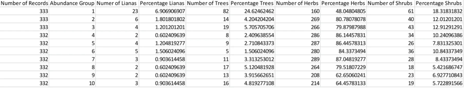
The aggregated data containing all North and South Carolina species in CVS plots was ranked according to large scale abundance (how many plots each species occurred in). This ranked list was divided into 10 equal groups, each containing about 332 species. The first group contained the 333 most abundant species (Abundance Group 1), the second group the 333 next most abundant species and so on. Using these groups, the percentage of each group that consisted of lianas, trees, herbs and shrubs was
8
abundance group). In addition, a multinomial regression model was fit to determine if plot abundance of species was a significant predictor of growth form (see appendix 1 for R code).
Ecological Amplitude Comparisons
The CVS plot data set has information on several different soil properties as recorded for each plot. For each species an aggregate of all the different soil property values for each of the plots that that species occurred in was created. From this aggregation, the 25th and 75th percentile of these soil property
values were calculated (these values were used instead of maximums and minimums in order to avoid outliers driving the data). The difference between the 75th and 25th percentiles was then determined for
each species (this value will be referred to as the range). These values represent a proxy for ecological amplitude. These ranges were then compared across growth forms to determine if certain growth forms had consistently larger or smaller ranges. For each growth form these ranges were then plotted against percent of plot occupied to determine whether having broader or narrower ranges for resource use/environmental tolerance influenced abundance.
RESULTS
Species Abundance Distribution
9
Small and Large Scale Abundance
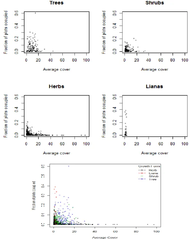
Contrary to the bulk of the literature, there did not seem to be a pattern between small and large scale abundance for the North and South Carolina CVS flora. Graphs of fraction of plots occupied and average cover show that herbs and shrubs run a wide range of cover values but never exceed 30% of plots covered (Fig. 2). Lianas, on the other hand, have consistently low cover (never more than 5%) but cover
10
a wide range of fraction of plots occupied. Trees cover a wide range of both values, remaining slightly less abundant regionally (fraction of plots occupied) than lianas, but much more abundant locally (average cover).
11
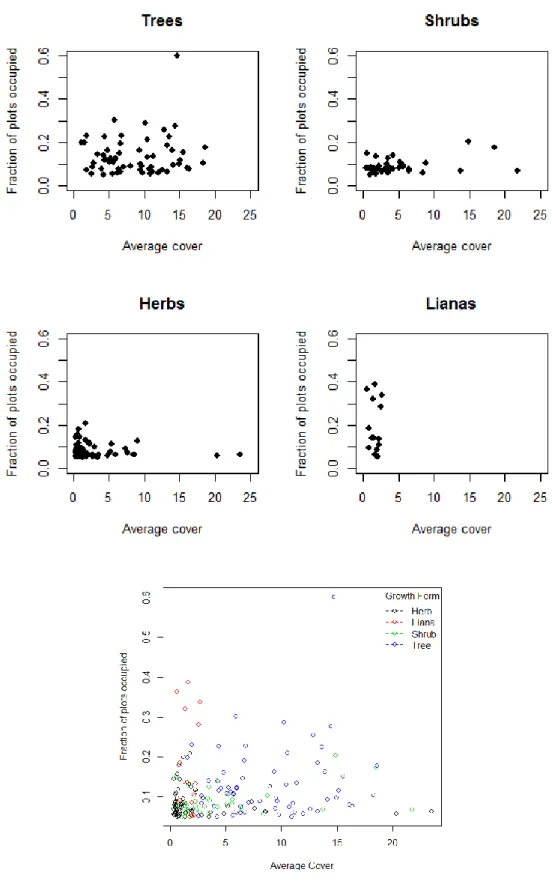
Figure 3 restricts the data to plants that only occur in 5% or more of plots in order to more clearly illustrate these patterns.
12
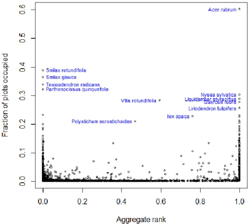
It is important to note, however, that these average cover values do not correct for plant size. As such a few large trees could have an equivalent cover value to numerous herbs even though the herbs would clearly have more individuals. The aggregation of ranks method takes into account the plot community in which a species occurs. It is a measure of a species cover relative to all of the other species in a plot and thus approximates dominance rather than raw percent cover. When this method was considered, a different pattern was discovered, although still not a positive correlation. Looking at the flora in general (Fig. 4), this comparison reveals two peaks. Species are mostly concentrated at low plot occupancy levels, but are able to reach higher fractions of plots occupied when they either 1) have low cover values compared to others, or 2) are very dominant in the plots that they occur in. Many lianas congregate in this first group, indicated by the spike on the left, whereas many trees congregate in this second group, indicated by the spike on the right.
13
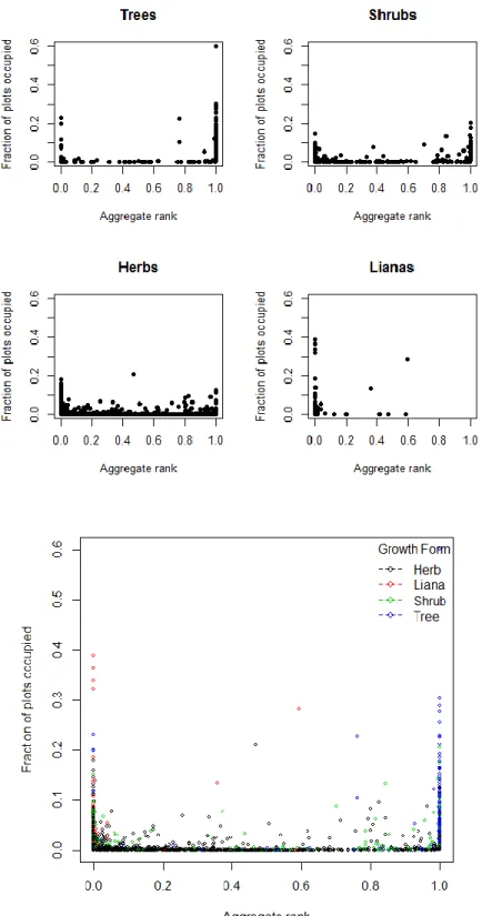
By growth form (Fig. 5), herbs and shrubs congregate at low proportions of plots occupied, trees show a large spike where proportion plots occupied and aggregate rank are both high and lianas show a large spike where the proportion plots occupied is high but aggregate rank is low.
14
Seedling/Non-Seedling Analysis
From a map of liana richness in all CVS plots in North and South Carolina one might expect a latitudinal gradient whereby lianas are most abundant and speciose at lower latitudes and decrease in richness as latitude increases. This does not appear to be the case for North and South Carolina lianas. Instead, liana richness is concentrated in the northeast, in plots that occur along the floodplain of the Roanoake River. Patterns of just seedling lianas and just non-seedling lianas track this same pattern (see appendix 2 for maps). One concern raised about the high abundance of lianas in the flora is that it might be inflated by high proportion of seedlings that don’t necessarily indicate establishment in a given plot. Based on the values of total seedling and non-seedling richness for the CVS plots, non-seedlings constitute 77.19% of all lianas diversity, whereas seedlings constitute 22.81% of all liana diversity. This unremarkable percentage of seedlings and the similarity of the geographic distribution of the total richness and seedling richness suggest that plots do not have artificially inflated liana richnesses.
Growth Form Abundance Comparison
15
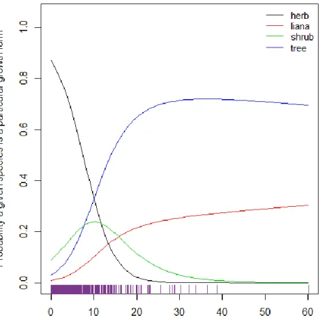
A multinomial regression model fitted to the data describes a similar pattern. Abundance (represented by percent of plots occupied) was used as a predictor of the multinomial response variable growth form (consisting of 4 levels: herb, liana, shrub and tree). Herb was taken to be the reference group. This model outperformed the null with AICs of 3615.951 and 3303.389, respectively. The Pr(Chi) value of an ANOVA test comparing the null and multinomial models indicated that the percent of plots occupied predictor was highly significant (p<0.0001). The odds ratios and 95% confidence intervals of this model are displayed in Table 3. Herb was taken as the reference group for this model. The odds ratios thus indicate that a 1 percent increase in percent plots occupied causes a 1.41 times increase in the odds of being a liana over being an herb, a 1.21 times increase in the odds of being a shrub over being an herb and a 1.40 times increase in the odds of being a tree over being an herb. Put another way, given a Table 2: Growth Form Groups with Abundance Breakdowns
Percentages represent the percent of the specific growth form that is found in each abundance group. For example, 42.6% of all lianas are found in the first abundance group.
Abundance Group Percentage of All Lianas Abundance Group Percentage of All Trees Abundance Group Percentage of All Herbs Abundance Group Percentage of All Shrubs 1 42.59259259 1 42.26804124 1 6.341656758 1 18.59756098 2 11.11111111 2 7.216494845 2 10.66191042 2 12.19512195 3 7.407407407 3 9.793814433 3 10.54300436 3 13.1097561 4 3.703703704 4 4.12371134 4 11.33571145 4 10.36585366 5 7.407407407 5 4.639175258 5 11.37534681 5 7.926829268 6 9.259259259 6 2.577319588 6 11.09789933 6 10.97560976 7 5.555555556 7 5.670103093 7 11.45461752 7 8.536585366 8 3.703703704 8 8.762886598 8 10.46373365 8 5.487804878 9 3.703703704 9 6.701030928 9 8.244153785 9 7.012195122 10 5.555555556 10 8.24742268 10 8.481965914 10 5.792682927
Table 1: Abundance Groups with Growth Form Breakdowns
Top row represents the top 333 most abundant species, the most abundant group. Percentages represent the percent of the specific abundance group that consists of the specific growth form. For example, 6.9% of the first abundance group is made up of lianas
16
species A with abundance X% plots occupied and species B with (X+1)% plots occupied, the odds that species B will be a liana over an herb is 1.41 times the odds that species A will be a liana over an herb. Thus, we can see that as abundance increases, the probability of being woody (and especially of being a tree or liana) increases.
These probabilities are displayed graphically in Figure 6. As the percent of plots occupied increases, the probability of a particular species being a liana or tree increases rapidly and then levels off. Lianas level off around 20% plots occupied at 0.2 probability, but continue to increase slightly afterward reaching an ultimate probability around 0.3 for 60% plots occupied. Trees level off around 20% plots occupied at about 0.7 probability and then decrease slightly for the remaining percentages. The probability of being an herb drops off rapidly; by 20% plots occupied the probability of being an herb is nearly zero and stays there for all higher abundances. Shrubs exhibit a more normal distribution, reaching peak probability at 10% plots occupied (Fig. 6).
Table 3: Odds Ratios of Multinomial Regression Model Estimate 2.50% 97.50%
17
Ecological Amplitudes Comparison
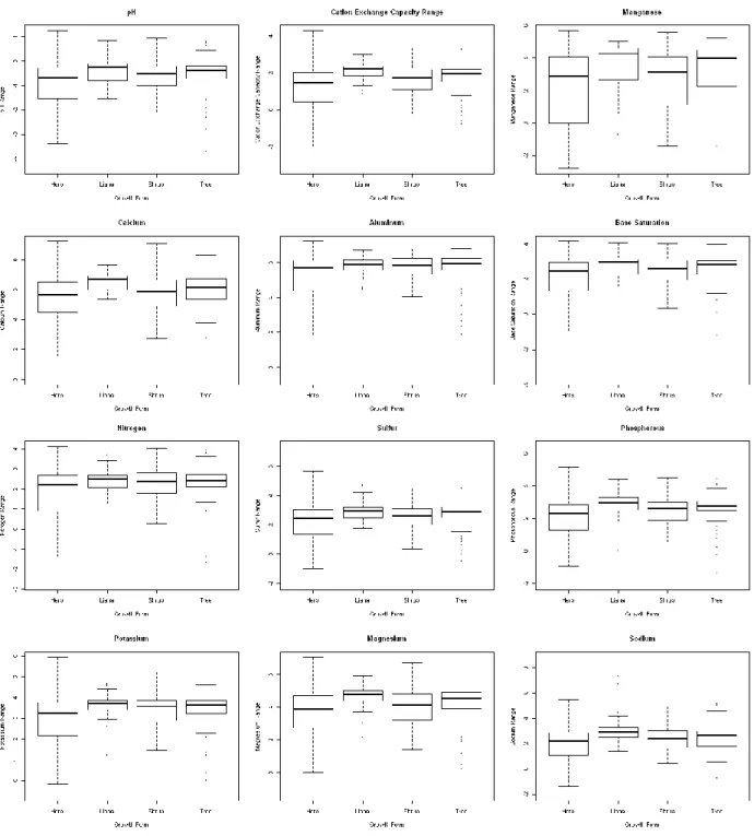
The differences between the 3rd and 1st quartile of a variety of soil properties (pH, cation exchange
capacity, Manganese, Calcium, Aluminum, Nitrogen, Sulfur, Phosphorus, Potassium, Magnesium, Sodium and base saturation) were calculated and will be referred to as ranges. This was done so that outliers would not drive the data as would be a risk if maximum and minimum values were used. Figure 7 shows that lianas and trees consistently had larger ranges for these soil properties than did herbs,
18
indicating that these woody taxa generally have a larger range of soil conditions in which they can thrive i.e. larger ecological amplitude/niche breadth/habitat generalism.
19
20
All of the significant predictors show an increase in proportion of plots occupied with range up until a certain peak after which proportion plots occupied drops off. Figure 7 indicates that trees and lianas have overall larger ranges for these soil properties, whereas herbs have overall smaller ranges with a handful of exceptionally large ranges. Figure 8 shows that lianas and trees cluster around this peak of proportion plots occupied. The tail that drops off after this peak consists of the larger ranges of these herb outliers. Since these herbs with large ranges do not show the large proportion of plots occupied that would be expected, it seems as if there is another factor driving the phenomenon of woody taxa having higher abundances than herbaceous taxa.
DISCUSSION
Results indicate that woody taxa (particularly trees and lianas) are indeed more abundant (as measured by percent of plots occupied by a particular species) than herbaceous taxa in the North and South Carolina CVS flora. Lianas and trees both had the bulk of their species (nearly 50%) aggregated in the top tier of abundance, with this percentage decreasing as abundance group decreased. Herbs had a more spread-out pattern with no one abundance class containing a significant percentage of species. A multinomial regression model demonstrated a similar pattern: as abundance (percent of plots occupied) increased, the probability of being woody (and especially of being a tree or liana) increased (Fig. 6). Maps of total richness of lianas, just seedling liana richness and just non-seedling liana richness show a similar pattern, with richness being highest in the Piedmont and the northeast corner of North Carolina
21
(Appendix 2). None of the maps showed a latitudinal gradient (decreasing richness with latitude) as might be expected. The fact that non-seedling richness is highest in the same places as total richness indicates that there are not plots where a high proportion of seedlings are artificially driving up the richness values while not actually establishing. This along with the fact that seedlings only contribute an unremarkable 23% to liana richness dispels some fears about potential lack of liana establishment in plots.
22
scales of heterogeneity, but more likely is a factor of trees being generally larger than the other growth forms and thus having higher cover values per same number of individuals. It may also be the case that liana cover is underrepresented due to overhead cover not being accurately accounted for in which case lianas might exhibit a pattern more like that shown by trees. A comparison of proportion plots occupied and aggregate rank abundance for the flora in general revealed two peaks. Species are mostly
concentrated at low plot occupancy levels, but are able to reach higher fractions of plots occupied when they either 1) have low cover values compared to others, or 2) are very dominant in the plots that they occur in. We can see 1) with Smilax rotundifolia, Smilax glauca, Toxicodendron radicans and
Parthenocissus quinquefolia which occur in a high percentage of plots but are never very dominant and 2) with the ubiquitous Acer rubrum which occurs in a high percentage of plots and is highly dominant in the plots it occupies (Fig. 4). Strikingly, the entire top portion of the left tail consists of lianas, whereas the entire top portion of the right tail consists of trees. When the flora is broken down into growth forms (Fig.5) we can see these same patterns. Herbs and shrubs concentrate mainly at low fractions of plots occupied with small spikes at high and low local dominance. Trees have a large spike where average cover and fraction of plots occupied are both high. Lianas have a similar spike, but where average cover is low and fraction of plots occupied is high. It is worth noting again, however, that trees are generally larger than lianas and thus would have higher cover values for the same number of individuals—that may be what is driving this last pattern. Regardless, however, here we have more graphical evidence that lianas and trees tend to inhabit higher numbers of plots.
23
properties (pH, cation exchange capacity, Manganese, Calcium, Aluminum, Potassium, Magnesium and base saturation) are significant predictors of proportion of plots occupied.
Figure 8 displays the relationship between soil property ranges and proportion of plots occupied. All of the significant predictors show an increase in proportion of plots occupied with range up until a certain peak after which proportion plots occupied drops off. Figure 7 indicates that trees and lianas have overall larger ranges for these soil properties, whereas herbs have overall smaller ranges with a handful of exceptionally large ranges. Figure 8 shows that trees and lianas cluster around this peak of
proportion of plots occupied. The tail that drops off after this peak consists of the larger ranges of these herb outliers. Since these herbs with large ranges do not show the large proportion of plots occupied that would be expected, it seems as if having a large range for one of these individual soil properties does not translate directly into higher abundance. It is still true that lianas and trees have higher abundance and, on average, higher ranges for all of these soil properties. What we may be seeing then, is a trend whereby lianas and trees having high ranges for a number of soil properties (again, high ecological amplitude) contributes to higher abundance whereas a specific herb having a broad range for one or a few soil properties does not. Identification of specific species on these graphs reveals that the herb species constituting these long right tails of wide range and low proportion plots occupied are different for each soil property, whereas the same species of trees and lianas occur at these high range widths across all soil properties.
24
studies that contain both woody and herbaceous taxa and investigate the drivers of the abundance of each. Walker and Langridge 1997, Breshars and Barnes 1998, Brown and Archer 1990, Daly et al. 2000, Dodd et al. 1998, Knoop and Walker 1985, Lauenroth et al. 1993 have all suggested—drawing from Walter’s two-layer theory—that the ratio of subsoil to top soil moisture is a significant determinant of woody: herbaceous biomass ratio (specifically woody: grass biomass). High amounts of subsoil moisture across North and South Carolina could therefore contribute to an overabundance of woody taxa that are able to utilize these resources, but unfortunately the CVS database does not contain this type of data.
The relationship between vessel diameter and susceptibility to cavitation by freezing found by Davis et al. (1999) runs contrary to the pattern we see in the North and South Carolina CVS data. We would expect that woody taxa, and particularly lianas, with their larger vessel diameters would be vulnerable to cavitation by freezing and therefore less abundant in areas prone to low temperatures and freezing, such as the mountains.
Lianas, as species that eventually climb, have the potential to invest less resource in support and more resource in light gathering, thereby ‘poaching’ light from other species with minimal self-investment. This life style habit of lianas could give them a competitive advantage over other species, thus helping explain their abundance in the flora. This phenomenon has been studied in tropical forests.
25
Another consideration in the saga of woody vs. herbaceous abundance is that of seed dispersal. It has been oft cited that niche assembly (i.e. habitat generalism/specialism) and dispersal ability are the main drivers of plant distribution with some studies claiming niche assembly as the most important factor (Tuomisto et al. 2003; Jones et al. 2006, Thompson 1999) and some claiming dispersal as the most important (Hubbell 2001; Nekola and White 1999). Recently many studies have posited that the relative importance of niche assembly and dispersal may vary by plant type, spatial scale and region (Pärtel et al. 1996; Zobel 1997; Gravel et al. 2006; Normand et al. 2006; Pärtel and Zobel 2006; Legendre et al. 2009). Unfortunately, data limitations prohibited a clear investigation into woody vs. herbaceous seed
dispersal.
It is recommended that further research be done on subsoil vs. top soil moisture and its effects on woody vs. herbaceous abundance, light competition and ‘poaching’ by lianas and differences between dispersal abilities of woody and herbaceous taxa in order to more definitely explain the high abundance of woody species in the North and South Carolina taxa.
CONCLUSION
1) Lianas and trees are more abundant than herbaceous species in the North and South Carolina CVS data.
2) Lianas and trees have wider ranges than herbaceous species for most soil properties which suggests that they have larger ecological amplitudes.
26
4) This indicates that the additive effect of having numerous large soil ranges might be the key and/or that there are other factors at play in explaining tree and liana overabundance.
WORKS CITED
Antos, Joseph A. 1988. Underground Morphology and Habitat Relationships of Three Pairs of Forest Herbs. American Journal of Botany 75: 106-113.
Ayensu, Edward S., and William Louis Stern. 1964. Systematic anatomy and ontogeny of the stem in Passifloraceae. Contr. U.S> Herbarium 34: 45-71.
Bamber, RK. 1984. Wood anatomy of some Australian rainforest vines. Proceedings of Pacific Regional Wood Anatomy Conference 1: 214-221.
Bock, Carl E., and Robert E. Ricklefs. 1983. Range Size and Local Abundance of Some North American Songbirds: A Positive Correlation. The American Naturalist 122.2: 295.
Breshears, David D. , and Fairley J. Barnes. 1999. Interrelationships between plant functional types and soil moisture heterogeneity for semiarid landscapes within the grassland/forest continuum: a unified conceptual model. Landscape Ecology 14: 465-478.
Brown, James H.. 1984. On The Relationship Between Abundance And Distribution Of Species. The American Naturalist 124.2: 255.
Brown, Joel R., and Steve Archer. 1990. Water Relations of a Perennial Grass and Seedling vs Adult Woody Plants in a Subtropical Savanna, Texas. Oikos 57.3: 366. Print.
27
Carlquist, Sherwin John. 1975. Ecological strategies of xylem evolution. Berkeley: University of California Press.
Cole, Elizabeth C., and Michael Newton. 1986. Nutrient, moisture, and light relations in 5-year-old Douglas-fir plantations under variable competition. Canadian Journal of Forest Research 16.4: 727-732.
Daly, Christopher, Dominique Bachelet, James M. Lenihan, Ronald P. Neilson, William Parton, and Dennis Ojima. 2000. Dynamic Simulation Of Tree-Grass Interactions For Global Change Studies.
Ecological Applications 10.2: 449-469.
Devineau, Jean-Louis. 2005. Generalist versus specialist: a contrasted sociology of woody and
herbaceous species in a fallow-land rotation system in the West African savanna (Bondoukuy, Western Burkina Faso). Phytocoenologia 35.1: 53-78.
Dodd, M. B., W. K. Lauenroth, and J. M. Welker. 1998. Differential water resource use by herbaceous and woody plant life-forms in a shortgrass steppe community. Oecologia 117.4: 504-512. Ewers, F. W., J. B. Fisher, and S.-T. Chiu. "Water Transport in the Liana Bauhinia fassoglensis (Fabaceae).
1989. Plant Physiology 91.4: 1625-1631.
Ewers, FW. 1985. Xylem structure and water conduction in conifer trees, dicot trees, and lianas.
International Association of Wood Anatomists 6: 309-317.
Fowler, Simon V., and John H. Lawton. 1982. The effects of host-plant distribution and local abundance on the species richness of agromyzid flies attacking British umbellifers. Ecological Entomology
7.3: 257-265.
Gaston, Kevin J., and John H. Lawton. 1990. Effects of Scale and Habitat on the Relationship between Regional Distribution and Local Abundance. Oikos 58.3: 329.
28
and neutrality: the continuum hypothesis. Ecology Letters 9.4: 399-409.
Guo, Qinfeng, and Robert E. Ricklefs. 2000. Species richness in plant genera disjunct between temperate eastern Asia and North America. Botanical Journal of the Linnean Society 134.3: 401-423. Hanski, Ilkka. 1982. Dynamics of Regional Distribution: The Core and Satellite Species Hypothesis. Oikos
38.2: 210.
Hawkins, Bradford A., Miguel A. Rodriguez, and Stephen G. Weller. 2011. Global angiosperm family richness revisited: linking ecology and evolution to climate. Journal of Biogeography 38.7: 1253-1266.
Hellkvist, J., G. P. Richards, and P. G. Jarvis. 1974. Vertical Gradients of Water Potential and Tissue Water Relations in Sitka Spruce Trees Measured with the Pressure Chamber. The Journal of Applied Ecology 11.2: 637.
Hodgson, J.G.. 1986. Commonness and rarity in plants with special reference to the Sheffield flora Part I: The identity, distribution and habitat characteristics of the common and rare species. Biological Conservation 36.3: 199-252.
House, Joanna I., Steve Archer, David D. Breshears, and Robert J. Scholes. 2003. Conundrums in mixed woody-herbaceous plant systems. Journal of Biogeography 30.11: 1763-1777.
Hubbell, Stephen P.. 2001. The unified neutral theory of biodiversity and biogeography. Princeton: Princeton University Press.
Jones, Mirkka M., Hanna Tuomisto, David B. Clark, and Paulo Olivas. 2006. Effects of mesoscale
environmental heterogeneity and dispersal limitation on floristic variation in rain forest ferns.
Journal of Ecology 94.1: 181-195.
29
African Savanna. The Journal of Ecology 73.1: 235.
Kunin, William E., and Kevin J. Gaston. 1993. The biology of rarity: Patterns, causes and consequences.
Trends in Ecology and Evolution 8.8: 298-301.
Lauenroth, W.k., D.l. Urban, D.p. Coffin, W.j. Parton, H.h. Shugart, T.b. Kirchner, and T.m. Smith. 1993. Modeling vegetation structure-ecosystem process interactions across sites and ecosystems.
Ecological Modelling 67.1: 49-80.
Lawton, John H.. 1993. Range, population abundance and conservation. Trends in Ecology and Evolution
8.11: 409-413.
Legendre, Pierre, and Eugene Gallagher. 2001. Ecologically meaningful transformations for ordination of species data. Oecologia 129.2: 271-280.
Mcnaughton, S. J., and L. L. Wolf. 1970. Dominance and the Niche in Ecological Systems. Science
168.3930: 455-455.
Morris, LA, SA Moss, and WS Garbett. 1993. Competitive Interference Between Selected Herbaceous and Woody Plants and Pinus taeda L. During Two Growing Seasons Following Planting. Forest Science 39.1: 166-187.
Neilson, RP. 1986. High resolution climatic analysis and south west biogeography. Science 232: 27-34. Nekola, Jeffrey C., and Peter S. White. 1999. The distance decay of similarity in biogeography and
ecology. Journal of Biogeography 26.4: 867-878.
Normand, Signe, Jaana Vormisto, Jens-Christian Svenning, Caesar Grandez, and Henrik Balslev. 2006. Geographical and environmental controls of palm beta diversity in paleo-riverine terrace forests in Amazonian Peru. Plant Ecology 186.2: 161-176.
Oosting, Henry J.. An Ecological Analysis of the Plant Communities of Piedmont, North Carolina.
30
Pärtel, Meelis, Martin Zobel, Kristjan Zobel and Eddy van der Maarel. 1996. The Species Pool and Its Relation to Species Richness: Evidence from Estonian Plant Communities. Oikos 75: 111-117. Pärtel, Meelis and Martin Zobel. 2006. Small-scale plant species richness in calcareous grasslands
determined by the species pool, community age and shoot density. Ecography 22.2: 153-159. Peet, Robert, Michael Lee, Forbes Boyle, Thomas Wentworth, Michael Schafale, and Alan Weakley.
2012. Vegetation-plot database of the Carolina Vegetation Survey. Biodiversity and Ecology 4: 243-253.
Qian, H., Z. Hao, and J. Zhang. 2014. Phylogenetic structure and phylogenetic diversity of angiosperm assemblages in forests along an elevational gradient in Changbaishan, China. Journal of Plant Ecology 7.2: 154-165.
Rapoport, E. H., and D. W. Shimwell. 1983. Areography. Geographical Strategies of Species.. The Journal of Ecology 71.3: 1037.
Ricklefs, Robert E., and George W. Cox. 1978. Stage of Taxon Cycle, Habitat Distribution, and Population Density in the Avifauna of the West Indies. The American Naturalist 112.987: 875.
Ricklefs, Robert E., and Roger Earl Latham. 1992. Intercontinental Correlation of Geographical Ranges Suggests Stasis in Ecological Traits of Relict Genera of Temperate Perennial Herbs. The American Naturalist 139.6: 1305.
Schultz, H. R., and M. A. Matthews. 1988. Resistance to Water Transport in Shoots of Vitis vinifera L. : Relation to Growth at Low Water Potential. Plant Physiology 88.3: 718-724.
Thompson, Ken, Kevin J. Gaston, and Stuart R. Band. 1999. Range size, dispersal and niche breadth in the herbaceous flora of central England. Journal of Ecology 87.1: 150-155.
Tuomisto, H.. 2003. Dispersal, Environment, and Floristic Variation of Western Amazonian Forests.
31
Tyree, M. T., and J. S. Sperry. 1988. Do Woody Plants Operate Near the Point of Catastrophic Xylem Dysfunction Caused by Dynamic Water Stress? : Answers from a Model. Plant Physiology 88.3: 574-580.
Van Vliet, GJCM. 1981. Wood anatomy of the palaeotropical Melastomataceae. Blumea 27: 395-462. Walker, Brian, and Jenny Langridge. 1997. Predicting savanna vegetation structure on the basis of plant
available moisture (PAM) and plant available nutrients (PAN): a case study from Australia.
Journal of Biogeography 24.6: 813-825.
Walter, Heinrich. 1971. Ecology of tropical and subtropical vegetation. New York: Van Nostrand Reinhold Co..
Welle, BJH. 1985. Differences in wood anatomy of lianas and trees. International Association of Wood Anatomists 6: 70.
Willis, J. C.. 1970. Age and area [A study in geographical distribution and origin of species] By J.C. Willis. London: Cambridge University Press.
Zobel, Martin. 1997. The relative of species pools in determining plant species richness: an alternative explanation of species coexistence? Trends in Ecology and Evolution 12.7: 266-269.
APPENDICES
Appendix 1: R Code
Aggregation of Ranks
library(RobustRankAggreg)
32
# obtain species names by plot
list.names <- split(species.sub$updatedTaxonName, species$OBSERVATION_ID)
# obtain cover values by plot
list.cover <- split(species$maxCvr, species$OBSERVATION_ID)
num.plots <- length(list.cover)
# sort species in each plot by their cover values breaking ties randomly
plot.list <- sapply(1:num.plots, function(x)
as.character(list.names[[x]])[order(rank(list.cover[[x]], ties.method="random"), decreasing=T)])
# obtain ranks in each plot
r3 <- rankMatrix(plot.list, full = TRUE)
# obtain aggregate ranks of species across plots
out.rank2 <- aggregateRanks(rmat = r3)
# give more prevalent species the higher scores
out.rank2$Score <- 1-out.rank2$Score
out.rank2
}
# initial run
out.rank3 <- random.order()
# next 25 random tie breaking runs
for(i in 1:25) {
# obtain aggregate ranks
out.rank3a <- random.order()
# change name of Scores
names(out.rank3a)[2] <- paste("Score", i, sep='')
# add to previous ranked species
out.rank3 <- merge(out.rank3, out.rank3a)
}
33
# obtain aggregate ranks
out.rank3a <- random.order()
# change name of Scores
names(out.rank3a)[2] <- paste("Score", i, sep='')
# add to previous ranked species
out.rank3 <- merge(out.rank3, out.rank3a)
}
for(i in 51:75) {
# obtain aggregate ranks
out.rank3a <- random.order()
# change name of Scores
names(out.rank3a)[2] <- paste("Score", i, sep='')
# add to previous ranked species
out.rank3 <- merge(out.rank3, out.rank3a)
}
for(i in 76:100) {
# obtain aggregate ranks
out.rank3a <- random.order()
# change name of Scores
names(out.rank3a)[2] <- paste("Score", i, sep='')
# add to previous ranked species
out.rank3 <- merge(out.rank3, out.rank3a)
}
# obtain the mean aggregate ranks
final.rank <- data.frame(Name=out.rank3$Name,
Score=apply(out.rank3[,2:ncol(out.rank3)], 1, mean))
# obtain fraction of plots occupied by each species
num.plots <- tapply(species$OBSERVATION_ID, species$updatedTaxonName, function(x) sum(x>0))
34
plot.fraction <- num.plots/total.plots
out.plot2 <- data.frame(Name=names(plot.fraction), plot.rank=plot.fraction)
# combine the two results
out.both2 <- merge(out.plot2, final.rank)
Multinomial Model
species<-read.csv('C:/Users/orndahl/Documents/Katie/Thesis/kmo_aggregate_growth _form.csv', header=T)
table(species$new_growth_form_clean)
# remove rare subshrubs, nonvascular plants and mistakes
species.sub <- species[species$new_growth_form_clean %in% c('Herb', 'Liana', "Shrub", "Tree"),]
# fix growth form levels
species.sub$new_growth_form_clean <- factor(species.sub$new_growth_form_clean)
# create percentages rather than fractions
species.sub$percentplots<-species.sub$plotrank*100
# fit null model
library(nnet)
nullmod <- multinom(new_growth_form_clean~1, data=species.sub)
# fit test multinomial model
abundmod <- multinom(new_growth_form_clean~percentplots, data=species.sub)
# test significance of predictor
anova(nullmod, abundmod)
# calculate odds ratios with herb as reference group
out.conf <- confint(abundmod)
data.frame(est=exp(coef(abundmod)[,2]), t(sapply(1:3, function(x) exp(out.conf[2,,x]))))
35
herb.prob <- function(x)
1/(1+exp(coef(abundmod)[1,1]+coef(abundmod)[1,2]*x)+exp(coef(abundmod) [2,1]+coef(abundmod)[2,2]*x)+exp(coef(abundmod)[3,1]+coef(abundmod)[3, 2]*x))
liana.prob <- function(x)
exp(coef(abundmod)[1,1]+coef(abundmod)[1,2]*x)/(1+exp(coef(abundmod)[1 ,1]+coef(abundmod)[1,2]*x)+exp(coef(abundmod)[2,1]+coef(abundmod)[2,2] *x)+exp(coef(abundmod)[3,1]+coef(abundmod)[3,2]*x))
shrub.prob <- function(x)
exp(coef(abundmod)[2,1]+coef(abundmod)[2,2]*x)/(1+exp(coef(abundmod)[1 ,1]+coef(abundmod)[1,2]*x)+exp(coef(abundmod)[2,1]+coef(abundmod)[2,2] *x)+exp(coef(abundmod)[3,1]+coef(abundmod)[3,2]*x))
tree.prob <- function(x)
exp(coef(abundmod)[3,1]+coef(abundmod)[3,2]*x)/(1+exp(coef(abundmod)[1 ,1]+coef(abundmod)[1,2]*x)+exp(coef(abundmod)[2,1]+coef(abundmod)[2,2] *x)+exp(coef(abundmod)[3,1]+coef(abundmod)[3,2]*x))
# graph probabilities
par(mar=c(5.1,6.1,1.1,1.1))
curve(herb.prob(x), xlim=c(0,60), ylim=c(0,1.05), xlab='Percent of plots occupied by a given species', ylab='Probability a given species is a particular growth form')
curve(liana.prob(x), add=T, col=2)
curve(shrub.prob(x), add=T, col=3)
curve(tree.prob(x), add=T, col=4)
legend('topright', c('herb','liana','shrub','tree'), col=1:4, lty=1, bty='n', cex=.9)
rug(species.sub$percentplots, col='mediumorchid4')
Soil Properties Model
species.sub$percentplots<-species.sub$plotrank*100
linearmod<-lm(percentplots~pHrangeq+cecrangeq+Mnrangeq+Carangeq+Alrangeq+Nrangeq+ Srangeq+Prangeq+Krangeq+Mgrangeq+Narangeq+baseSaturationrangeq,
36
39