A hybrid Fire Fly and differential evolution algorithm for
optimization of a mixed repairable and non-repairable system
reliability problem
Shima, MohammadZadeh1*, SeyedJafar, Sadjadi 2
1
Department of Industrial Engineering, Science and Research Branch, Islamic Azad University, Tehran, Iran
2
Industrial Engineering Department, University of Science and Technology, Tehran, Iran [email protected], [email protected]
Abstract
In this paper, a hybrid meta-heuristic approach is proposed to optimize the mathematical model of a system with mixed repairable and non-repairable components. In this system, repairable and non-repairable components are connected in series. Redundant components and preventive maintenance strategies are applied for non-repairable and repairable components, respectively. The problem is formulated as a bi-objective mathematical programming model aiming to reach a tradeoff between system reliability and cost. By hybridizing a standard multi-objective fire fly (MOFA) and differential evolution (DE) algorithms, a powerful and efficient approach called MOF-DE algorithm which has inherited the advantages of the two algorithms is introduced to solve this problem. In order to achieve the best performance of MOF-DE, response surface methodology (RSM) is used to set proper values for the algorithm parameters. To evaluate the performance of the proposed algorithm, various numerical examples are tested and results are compared with methods like NSGA-II, MOPSO and standard MOFA. From the experiments, it is concluded that the performance of the MOF-DE algorithm is better than other methods at finding promising solutions. Finally, sensitivity analysis is carried out to investigate behavior of the proposed algorithm. Keywords: Meta-heuristics, Reliability, Firefly algorithm (FA), Differential evolution (DE), Multi-objective Optimization, Preventive Maintenance
1- Introduction
Reliability is a criterion for measuring performance of a system, and the larger and more complex a system the greater the cost due to poor and unreliable performance. Compensating for this cost can sometimes be impossible; therefore, the optimization reliability problem has been considered by many researchers. There are three approaches to increase the reliability of a system, 1) optimizing the system component reliability by adjusting the process parameters, 2) the use of redundant components in series, parallel or a combination, and 3) taking preventive maintenanceaction(Rigdon, 2008).Since the components of a system are repairable or non-repairable, the two types of problems in the field of reliability optimization are defined as redundancy allocation problems (RAP) and reliability centered *Corresponding author.
ISSN: 1735-8272, Copyright c 2017 JISE. All rights reserved Journal of Industrial and Systems Engineering
Vol. 10, special issue on Quality Control and Reliability, pp.59 – 77 Winter (February) 2017
maintenance (RCM). Most studies consider just one of the problems and provide a method to solve it. For examples; Heungseob and Pansoo developed stochastic models to design and analyze the time-dependent reliability of non-repairable systems with heterogeneous components using a structured Markov chain (Heungseob & Pansoo, 2017). To analyze and compare the age and block replacement policies, a numerical analysis technique was proposed by (Rebaiaia, Ait-Kadi, Rahimi, & Jamshidi, 2016). In real world, a system may compose of many components with uncertain values of reliabilities. Soltani et al have used a robust optimization approach to solve the redundancy allocation problem (RAP) in series parallel systems with component mixing where uncertainty exists in components’ reliabilities.(Soltani, Safari, & Sadjadi, 2015). Salmasnia et al (Salmasnia, Ameri, & Niaki, 2016)had proposed a method based on the robust loss function approach to solve the redundancy allocation problem. Few studies have examined both problems (RAP and RCM) simultaneously. However, in the real world systems are generally composed of both repairable and non-repairable components (Zoulfaghari, Hamadani, & Abouei Ardakan, 2014). In this study, a mathematical model of a system consisting of repairable and non-repairable components is developed. The time of reaching inherent availability for all components is considered to be less than the mission time so availability function reaches a constant. Omitting this limitation allows the mathematical model developed by Mohammad Zadeh Doghahe and Sadjadi (2015) (MohammadZadeh Dogahe & Sadjadi, 2015) to be used in this study. In their model cold and hot strategies are considered for redundant components.
A wide range of optimization problems in various fields of engineering that we face today, are complex and nonlinear. Hence, understanding and applying effective methods with reasonable cost and time, that provides the opportunity to find solutions with good quality, is important. The high computational cost and time in exact and approximate mathematical methods and sometimes their disability in solving these problems, has led to the emergence of new methods. Since nature is a good sample for optimization and evolution, these methods are inspired by nature and are called meta-heuristic methods. These methods are classified into three groups: Meta-heuristics based on gene transfer, Meta-heuristics based on interactions among individual insects and Meta-heuristics based on biological aspects of alive beings (Ruiz-Vanoye & Díaz-Parra, 2011). For example Genetic Algorithms belongs to the first category, Ant Colony, Honey Bees and Firefly Algorithms are the second category and Simulated Annealing, Tabu Search and Particle Swarm Optimization Algorithms fall into the third category. Although these methods does not guarantee an optimal answer, but based on evidence and experience in dealing with computational time and cost, they are evaluated efficient and considering their power and efficiency are widely applied in many optimizations fields.
Since in order to increase system reliability, cost, volume, weight and system down time due to maintenance also increase, in most recent studies, the problem is considered as two or multi-objective so that conflicting objectives such as system reliability, total cost, system downtime, volume and weight are optimized simultaneously. These problems are categorized as NP-Hard Problems (Chern, 1992) and to solve them, Meta-heuristics method has been used extensively. For example, Suman (Suman, 2003) has used simulated annealing algorithm and Zhao et al (Zhao, Liu, & Dao, 2007)have used ant colony algorithm to solve multi-objective reliability problems. In another study, Non-dominated Genetic algorithm (NSGA) has been used for identifying Pareto solutions set of multi-objective redundancy allocation problem (MORAP) and by using two approaches, pseudo-ranking scheme and data mining clustering; the best solutions have been selected by decision maker (Taboadaa, Baheranwalaa, & Coit, 2007). Also Kumar et al (Kumar, Izui, Yoshimura, & Nishiwaki, 2009)has used two well-known genetic algorithms known strength Pareto evolutionary genetic algorithm (SPEA2) and NSGA-II to optimize multi-level RAP. A penalty based cuckoo search (CS) algorithm was presented to solve the reliability e redundancy allocation problems (RRAP) with nonlinear resource constraints by Garg (Garg, 2015).He et al had developed basic artificial fish swarm algorithm by adding selection and crossover operators to solve large-scalereliability-redundancy allocation problem(RRAP). (He, Hu, Ren, & Zhang, 2015) In some studies, multi-objective problem is converted to a single-objective problem using weighted or penalty function technique and then are solved. Huang et al(Huang, Qu, & Zuo, 2009) argue that converting multi-objective problems to the single objective problems, reduce the number of optimal
solutions, therefore provided a multi-objective optimization algorithm combined with niched Pareto GA and a method of constraint handling, that solve the multi-objective problems without the need of penalty parameter in three steps: 1) searching forfeasiblesolutions2) choose the non-dominated solutionsand3) maintaining the diversity of solutions. Liang and Lo (Liang & Lo, 2010) in their study optimized MORAP problem with the use of multi-objective variable neighborhood search algorithm and a new selection strategy based on the balance between intensity and diversity. Also, another study of two-stage approach is used to solve MORAP (Li, Liao, & Coit, 2009). Such that at the first step, multiple objective evolutionary algorithm (MOEA) method to determine the Pareto set is applied and similar solutions using self-organizing map (SOM) are classified. In the second step, the effectiveness of solutions in each category is compared by data enveloping analysis (DEA).
Fire fly algorithm as a meta-heuristic optimization method was introduced in 2008 (Yang, 2010). The algorithm was first presented for single-objective and continues problems and in 2013 was developed to multi-objective Firefly algorithm (Yang, 2013). Sayadi et al. (2013) have used multi-objective firefly algorithm to solve the manufacturing cell formation problem. Noting that the solution space of the algorithm is continuous and problem variables are binary, sigmoid function is used to convert continuous to binary solutions. This algorithm is called discrete firefly algorithm (DFA). Another study has used DFA on multi-objective flow shop scheduling problem (Marichelvam, Prabaharan, & Yang, 2014). Li and Ye(Li & Ye, 2012) have used MOFA for optimizing production scheduling system with two objective of make span and machines vacancy rate target function. Gandomi et al. (2011) have used FA for mixed continuous and discrete structural optimization problems. RAP problem was solved using Firefly algorithm that was modified by combining with chaotic sequences. They showed the advantages of FA by comparing the results (Dos Santos Coelho, de Andrade Bernert, & Mariani, 2011). Other studies over the past five years using the FA algorithm have been reviewed by Yang and He (2013).
Also some studies in recent years have been conducted to compare FA algorithm with other Meta-heuristic algorithms, for example, Goel et al have used two algorithm inspired by particle intelligence for unconstrained problems optimization. They compared the performance of bat algorithm and fire fly algorithm and showed that FA has better results than BA (Goel, Gupta, & Goel, 2013). Chai-ead et al used fire fly and bees algorithms to solve noisy non-linear optimization problems and demonstrated that in these problems FA will provide better results (Chai-ead, Aungkulanon, & Luangpaiboon, 2011). Also using neural network and FA the process of cutting glass with water jet has been modeled and optimized (Amirabadi, Khalili, Foorginejad, & Ashoori, 2013).
This paper aims at using the new firefly improved algorithm to solve a bi-objective reliability problem of a combined system of repairable and non- repairable components using redundancy and maintenance strategies. Our work is presented in five sections. The first part is a review of the literature and past research. The second part presents the developed mathematical model of the reliability problem, and section three provides the conventional methodology of multi-objective firefly algorithms and the idea derived from differential evolution (DE) algorithm is described. In Section four numerical examples using the proposed algorithm are solved and the results are compared with basic MOFA, non-dominated sorting genetic algorithm (NSGA-II) and multi objective particle swarm optimization (MOPSO). Finally, the conclusions are presented.
Nomenclature
Indices and Parameters:
: indices for components of non-repairable subsystem
є {1, 2, . . . , }
́: indices for components of repairable subsystem
́ є {1, 2, . . . , }
: component type in non-repairable subsystem
є {1, 2, . . . , }
: number of available types for component : time counter є {1, 2, . . . , }
T: system mission time
m: number of inspections during each time unit
For non- repairable components:
: available budget to purchase redundant components
V, W: maximum allowed volume and weight wij: weight of type j of component i
vij: volume of type j of component i
: purchasing cost for type j of component i λij: failure rate of type j of component i
For repairable components: ́: repair cost for component ́ ́: replacement cost of component ́ ̅́: failure rate of component́ after repair
̿́: failure rate of component́at time zero and after each replacement
́: maximum allowed failure rate for component ́ !́:rate of increase in failure rate for repairable component ́
"#": failure rate of component ́ at period t
Decision variables:
$%&: number of components i with type j used as redundant
'́#: if repair is performed on subsysteḿ in period t equals 1; otherwise 0
'́́#: if component ́is replaced in period t equals 1; otherwise 0
2- Mathematical Formulation
In most research the system under study includes either repairable or non-repairable components, but in real world systems usually consist simultaneously of both repairable and non-repairable components. A new mixed integer nonlinear model of a system with both repairable and non-repairable components was introduced by Mohammad Zadeh Doghahe and Sadjadi (2015). Our model was formulated according to their model and the following assumptions.
• M + E subsystems consist of E non-repairable and M repairable subsystem connected in series.
• In order to increase system reliability parallel redundant components are applied to non-repairable parts and preventive maintenance actions are applied to repairable parts.
• Parameters related to non-repairable components including component failure rate, purchase price, weight and volume are specific and certain.
• Redundant components strategy is active. Also, redundant components can be selected from different types.
• A fixed amount of budget is available at time zero to purchase redundant components. Also, the total volume and weight of the non-repairable components are defined and limited.
• The repairable components failure rate increases with !in each period. The maximum allowed failure rate for each period is known ( ), ifa componentfailure ratebecomes more than the allowed value, it will be repaired or replaced at the first inspection.
• The repair and replacement cost of any component is determined and failure rates are calculated after each inspection according to equation (6).
• System mission time and the number of inspections during each period are determined.
Thus, the developed mathematical model of the problem with two objectives and seven constraints is formulated as follows:
($ R* + = - .1 − - 01 − 12345.# 6 7 8 9
:!
<452
9=
>
45 ?4
=
@
∈B
× - 12*3D́E#+F ́∈
(1)
G H* + = 6 6 * ́ × '́#+ ́ × '́́#+ ́=
JK
L=
(2) 6 6 M . $B
= ?4
= ≤ O (3)
6 6 P . $B
= ?4
= ≤ Q (4)
'́#+ '́́#≤ 1 ∀ ́ = 1, … , = 1, … , (5)
́#= 7 ́*#2 ++ !́8 × 71 − *'́#+ '́́#+8 + '́#× ̅́+ '́́#× ̿́ ∀ ́ = 1, … , = 1, … , (6)
́#≤ ́ ∀ ́ = 1, … , = 1, … , (7)
6 6 $ ×
?4
= B
=
≤ (8)
'́#∈ {0,1}, '́́#∈ {0,1}, $ ∈ UV (9) Equation (1) and (2) show the objectives of the problem, including maximizing reliability and minimizing costs. Repairable and non-repairable components are connected in series so the reliability of the system is obtained by multiplying the reliability of these two sections. It is assumed that the time-to-failure distribution function of non-repairable components are W:(GX * , Y+ (sum of working time of components which have Exponential failure distributions) (Coit, 2001),(Azaron, Katagiri, Kato, & Sakawa, 2005) and (Safari, 2012). Also, the reliability is calculated based on the distribution function of
O1 Z[:: \],3^ in the repairable section (Jardine & Buzacott, 1985), (Dieter, Pickard, & Bertsche, 2010) and (De Castro & Cavalca, 2006). The cost function is total cost of components repair and replacement during the system mission time, which should be minimized.
Constraints (3 and 4) explain that the total weight and volume of the assigned components to the non-repairable components should not exceed allowed weight and volume (V, W: maximum allowed volume and weight). Equation (5) states that components of the repairable section can be repaired or replaced only at inspection points and the constraints of Equation (6) determine the failure rate of each component in each period according to the type of action (replacement, repair or no action). Failure rate is increased by !́ if no repair or replacement action is taken on the component at period t, and is changed into ̅9" and
̿_́" if the component is repaired and replaced at period t, respectively. Constraint (7) determines the upper
limit of acceptable failure rate of each component in a period. Constraint (8) ensures that the total cost to purchase redundant components in the non-repairable section does not exceed the available budget and constraints, and (9) shows the range of problem decision variables.
3- Multi-Objective Fire Fly Algorithm
In this section, first the methodology of basic multi-objective fire fly algorithm (MOFA) is discussed then the improved algorithm, inheriting the superiority of both algorithms MOFA and differential evolution (DE), is offered.
3-1- Methodology
Swarm Intelligence is a new field of research that solves complex problems in reality by inspiring social behavior models of particles. By complex problems we mean problems that are seeking a minimum or maximum value of one or more objective functions in a D-dimensional space. Using traditional and exact methods to solve these problems requires high computational cost and time. Thus, swarm intelligence
algorithms were introduced to solve these problems. These algorithms find time and cost effective solutions near the optimal solution. The firefly algorithm is one of these methods.
The firefly algorithm was introduced by Xin-She Yangin (2007). This algorithm was inspired by the flashing behavior of fireflies to attract each other. Fireflies produce cold light with wavelengths from 510 to 670 nanometers. The two main functions of flashes in these insects are mating and attracting preys. The fireflies also use flashing lights as a defense against predators. Yang introduced the firefly algorithm by considering the following rules:
Fire flies attract each other regardless of their sex. With increasing distance, attractiveness will decrease.
The brightness of fire flies are defined according to the objective function.
Brightness (I) of each firefly at place x is defined as` *$+ ∝ b *$+ and attractiveness (β) is defined with respect to distance of firefly i from firefly j*W +. In addition, the light intensity decreases with distance from the light source, generally shown in the form of ` *W+ = `cdW where r is the distance from the source and `c is intensity at the source. In order to avoid singularity at r = 0 this equation, based on the Gaussian form, is approximated to equation `where` is the original light intensity and e is the fixed light absorption coefficient. e is a parameter describing the variation of the attractiveness and its value has a great impact on the speed of convergence and the FA performance. Attractiveness of a firefly, as mentioned, is proportional to light intensity, so attractiveness is calculated as equation (10):
Where f is attractiveness at r = 0. The distance between firefly i and firefly j at $ and $, respectively, based on the Cartesian distance is obtained as follows:
) 11 (
W = g$ − $ g = h67$,<− $,<8
i <=
Where $,< is the Y-th component of $% in spatial coordinate. Regarding the type of the problem, calculating distances can be defined differently. Equation (12) presents how the movement of firefly i towards firefly j (more attractive) is calculated:
(12)
$V = $ + f 12jk45l7$ − $ 8 + ] m
The second term of equation (12) is movement because of attraction and the third term is random movement where ] is a randomization parameter and n% is the vector of random numbers with a Gaussian or uniform distribution.
Yang has shown that this algorithm is more effective and more successful than other algorithms such as PSO and GA(Yang X. , Multiobjective Firefly Algorithm for Continuous Optimization, 2013).This method was first designed for continuous problems, but more recent studies have shown that it is also very efficient in discrete problems(Sayadi, Hafezalkotob, & Jalali Naini, 2013). Simplicity in understanding and implementation of the FA is the advantage of this algorithm compared to other similar algorithms. Below are some notes that represent the behavior of FA (Yang, 2010) in special cases referred to:
If f = 0 random walk biased is converted to simple random walk.
When γ → 0, it means that the attractiveness is constant at every distance and here FA becomes a special case of the PSO algorithm.
When γ → ∞, that means the attractiveness is almost zero and this is similar to random search method.
) 10 (
When G →∞ (number of fireflies), and ≫ 1 (number of iterations), then the algorithm FA will close to the global optima.
Large values for m indicate rapid decrease of light intensity with increasing distance. 3-2- Efficient Hybrid MOF-DE Algorithm
The mathematical model in this study is formulated as a bi-objective problem; therefore a multi-objective firefly algorithm (MOFA) is applied. FA was developed into MOFA by Yang (Yang, 2013). In his algorithm, the standard MOFA will be a random walk around the best point if no new non-dominated solutions are found after any iteration, meaning$#V = X∗#+ ]#m# where X∗# will be the best solution found. In this way, new solutions are generated. Yung has tried to present a more powerful approach for multi-objective optimization problems by developing MOFA.
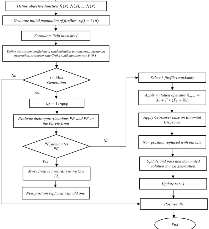
We have used a differential evolution algorithm (DEA) to empower standard MOFA and to propose an efficient hybrid MOF-DE algorithm. Our proposed algorithm uses crossover, mutation and selection operators derived from DEA when MOFA is unsuccessful in finding a new non-dominated solution in a given iteration. The difference between the MOF-DE proposed algorithm and standard MOFA is that the MOF-DE algorithm gives all solutions the same chance of being selected to generate new solutions and the optimal level is not a priority in the selection operation. The advantage of this idea is that the probability of getting trapped in a local optimum is reduced and with full random movements the possibility of searching a wide range of solution space is provided. Figure 1 shows the flowchart of the MOF-DE algorithm.
Simplicity, speed of convergence, accuracy, robustness and a small number of parameters are some advantages of DEA that have attracted the attention of many researchers (Das & Nagaratnam Suganthan,
End Yes
Apply mutation operator uvwx=
u + y ∗ *u + uz+
Apply Crossover base on Binomial Crossover
Start
New position replaced with old one Define objective function b *$+, b *$+, … , b<*$+
Generate initial population of fireflies $ * = 1: G+
Formulate light intensity I
Define absorption coefficient γ; randomization parameter], maximum generation, crossover rate Cr(0,1) and mutation rate F (0,1)
, = 1: Gpop
t < Max Generation
Evaluate their approximations PFi and PFj to the Pareto front
Move firefly i towards j using (Eq. 12)
PFj dominates PFi
New position replaced with old one No
No
Select 3 fireflies randomly
Yes
Update t=t+1 Update and pass non dominated
solution to next generation
Post results
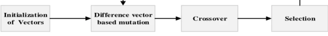
2011).This algorithm searches for the optimal global solutions in four main stages, as presented in figure 2.
Initialization of Vectors
Difference vector
based mutation Cross over Selection
Figure 2. DE Algorithm stages
First, the initial solution vector in D-dimensional space is randomly generated. In our proposed algorithm, the initial solutions of DE are selected among the solutions generated by MOFA. In the second stage, three vectors are selected randomly from the current population; the difference between two vectors is computed and then multiplied by F, a random number in the interval (0, 1) known as the control parameter. The result is added to a third vector. Equation (13) expresses this process.
(13)
u|
In order to enhance diversity of the solutions, across over operation is utilized in the third step. Two common methods that are used in the crossover operation are exponential and binomial. The binomial method is employed as a cross over operator in our proposed MOF-DE algorithm. At this point, the mutant solutions are combined with a target vector chosen among the existing solutions and new solution vectors are generated. Crossover rate (Cr) is also used as the control parameter similar to F. We set Cr based on the RSM result as explained in the next section. The last step is to determine whether the new or the pervious solution is chosen. If the new solution dominates the previous one, it replaces it; otherwise the pervious solution is retained in the population and other solutions are generated according to the mentioned procedure.
Since the variables of our problem are binary and integer and MOFA and DE algorithms find solutions in continuous space, round and sigmoid functions are used to convert real number to the integer and binary solutions. In the next section some numerical examples are employed, after setting algorithm parameters, to compare the proposed algorithm (MOF-DE)with the basic multi-objective firefly algorithm (MOFA), non-dominated sorting genetic algorithm (NSGA-II) and multi objective particle swarm optimization (MOPSO).
4- Numerical examples
In this section at first, the effective parameters on algorithms performance are first adjusted with the help of RSM and then using some numerical examples the proposed algorithm is compared to basic MOFA, NSGA-II and MOPSO algorithms. All algorithms are coded in MATLAB and the test problems have been solved on a PC with 4 GB RAM/1.80 GHz CPU.
4- 1- Tuning the Parameters
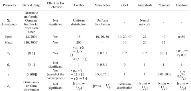
Identifying key algorithm parameters and setting their proper values greatly affects the performance of the algorithms. Table 1 reviews how parameters were set in the literature. Response surface methodology (RSM) was employed to determine the optimum value for our proposed algorithm. RSM is a mathematical and statistical technique that examines the relationship between one (or more) response variables and the set of parameters (input variables) influencing them. Using this method, the levels of parameters that optimize the response variables were identified (Najafi, Akhavan Niaki, & Shahsavar, 2009).
The main parameters of the MOF-DE algorithm are number of population (Npop), maximum iteration (Maxit), randomization parameter (∝ ), fixed light absorption coefficient (γ) and crossover rate (Cr). The upper and lower values for each parameter as well as the appropriate design of experiments should be determined before using the RSM. Central composite and Box-Behnken are two common designs. Table
2 shows the range of the input parameters that were specified based on the literature review. Design Expert 7 software was used to run RSM. A central composite design (CCD) with 8 center points and face-centered design was applied for the experiment. A set of 50 test problems were run to generalize the statistical results according to the design.
Table 1. FA parameters value in previous studies
Gandom Chai-ead Amirabadi Goel Marichelva Coelho Effect on FA
Behavior Interval Range Parameter - - Neural network - Uniform distribution Uniform distribution Not significant Distribute uniformly/ Generate fireflies far from each other X0 (Initial pop) n<50 40 27 10, 20, 40
10, 20, 50 15 Yes [2, 200] Npop 15 20 10 - 200 Yes [10, 3000] Maxit
0.01 L**
∝ 0.9#
[0,1] 0.2
0.2 0, 0.5, 1
∗ • . e* − 1+ × €1 − ] * − 1+•
Yes ‚0,1ƒ ∝ 1 1 1 0
0, 0.5, 1 1 Not significant [0, 1] f 1 √… d
0.5d…
[0.01,100] 1
1 0.5, 0.75, 1
∗ • . e* − 1+ × €1 − e* − 1+•
Yes (speed of the convergence)
‚0,100•ƒ e
€W(G‡ −
1 2d]
€W(G‡ −
1 2d]
€W(G‡ −
1 2d]
Gaussian distribution
€W(G‡ − 1 2d ]
€W(G‡ −
1 2d]
Not significant Gaussian or uniform distribution m
*1 ≤ • ,• ≤ 4 ** L: length of design variables (upper bound- lower bound)
Table 2. Range of the parameters
High Low Parameter 100 10 Npop 200 50 Maxit 0.9 0.1 ∝ 3 1 e 0.9 0.5 Cr
Next the response variables should be determined. As mentioned in the literature, there are two criteria to evaluate algorithm performance: i) Convergence to the Pareto set and ii) Diversity of the produced Pareto optimal set. Several metrics have been proposed to measure these two criteria (Yu & Gen, 2010). For example, the number of non-dominated solutions (NNS) is a convergence metric, and diversification metric (DM) and maximum spread metric (MS) are criteria of measuring diversity that are calculated in equations (14) and (15).
‰ = Š6 ($*‖$ − ' ‖+ Œ
=
• d
(14)
= Š 6* ($|Œ|=y bJ− G|Œ|= bJ+
JJ − yJJ v
J=
• d
(15) Where, ‖$ − ' ‖ is the Euclidean distance between the non- dominated solution $ and the non-dominated solution '(Khalili-Damghani, Abtahi, & Tavana, 2013). Letters M and N denote number of objective functions and number of the Pareto solutions, respectively,bJ is the m-th objective function
value for i-th number of the Pareto solution, and yJJ / yJJ vis the maximum/ minimum value of the m-th objective function.
In addition to the above metrics, computation time (CPU time) and the ranges of reliability and cost(difference between the maximum and minimum of generated solutions for objective functions), are also key measures to evaluate algorithm performance. Here NNS, CPU and solutions quality (SQ) are considered as response variables for comparing different designs. SQ is the weighted average of the DM, MS, reliability (b ) and cost (b ) measures that are calculated as follows:
• =M × •‰`‘ + M × •‰`M + M + M?+ Mz× •‰`’“+ M”× •‰`’l
z+ M” (16)
Where M , . . , M”the weight of each metric and RDI are is the relative deviation index that is calculated in equation (17). RDI is used to normalize raw data. After running the algorithm on a variety of designs, the obtained results are normalized using this index. In this study, M values are considered 1, 1, 2, and 2, respectively.
(17)
•‰` =|‰1• XG|O—W• c–9− 1• c–9|
c–9− 1• c–9| × 100
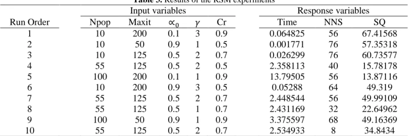
‰1• XGc–9 is the solution obtained for each design and 1•c–9 and O—W• c–9are the best and worst solutions obtained among all designs, respectively. RDI=0 indicates the best state and RDI=100 indicates the worst state. Some results of the RSM are presented in Table 3.
Table 3. Results of the RSM experiments
Input variables Response variables
Run Order Npop Maxit ∝ e Cr Time NNS SQ
1 10 200 0.1 3 0.9 0.064825 56 67.41568
2 10 50 0.9 1 0.5 0.001771 76 57.35318
3 10 125 0.5 2 0.7 0.026299 76 60.73577
4 55 125 0.5 2 0.5 2.358113 40 15.78178
5 100 200 0.1 1 0.9 13.79505 56 13.87116
6 10 200 0.9 3 0.5 0.05288 64 49.319
7 55 125 0.5 2 0.7 2.448544 56 49.99109
8 55 125 0.5 1 0.7 2.431169 32 22.64962
9 100 50 0.9 1 0.9 3.375597 68 49.16369
10 55 125 0.5 2 0.7 2.534933 8 34.8434
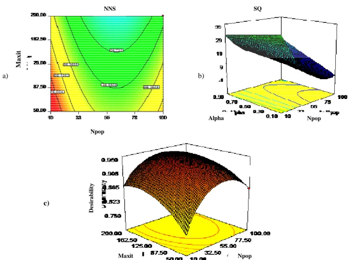
After performing the experiments, analysis of variance (ANOVA) is used to fit an adequate model to the experimental data and finally optimum values for the algorithm parameters are identified according to the desired response values. Contour and surface plots display how a response variable relates to two factors based on a model equation. For instance, the contour plot in Figure 3-aindicates that the highest NNS is obtained when the Npop level is medium (about 55 to 65) and Maxit level is about 160. This area appears in the green part of the plot. The surface plot (Figure 3-b) also shows that the highest SQ is obtained when the Npop level is medium and alpha (] ) level is high. Figure 3-c and Table 4 present the optimum values for the algorithm parameters that provide the highest desirability.
a)
c)
Figure 3. Counter and surface plots, a) NNS vs. Npop and Maxit, b) SQ vs. Npop and Alpha (
Table 4. Optimum value for parameters of MOF
* Resulted from RSM ** Mutation rate Value MOF-DE 60 *Npop 170 *Maxit. 0.9 *∝ 1 * e
0.9 *Cr
1
f
€W(G‡ / 1 2d • m NNS Npop M a x it D es ir a b il it y b)
Counter and surface plots, a) NNS vs. Npop and Maxit, b) SQ vs. Npop and Alpha ( Maxit and Npop
Optimum value for parameters of MOF-DE and other algorithms
** Mutation rate ***Cross over rate ****Cognitive and social learning factors
Value NSGA-II Value MOFA 100 Npop 50 Npop 200 Maxit 200 Maxit. 0.2 **Mr 0.25 ∝ 0.9 ***Cr 1 f 1 e
€W(G‡ / 1 2d • m
NNS SQ
Alpha
Npop Maxit
Counter and surface plots, a) NNS vs. Npop and Maxit, b) SQ vs. Npop and Alpha (] ), c) Desirability vs.
DE and other algorithms
***Cross over rate ****Cognitive and social learning factors
Value MOPSO Value 50 Npop 100 200 Maxit 200 0.1 Alpha 0.2 2 ****H 0.9 2 ****H Npop
b)
a)
d)
c)
f)
e)
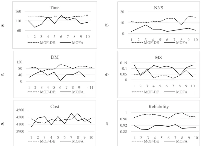
Figure 4. Comparing obtained results by proposed algorithm (MOF-DE) and standard MOFA
4-2- Evaluating Proposed Algorithm
In this section using a number of test problems, the proposed algorithm (MOF-DE) is compared with three well-known algorithms, standard MOFA, NSGA-II and MOPSO. Table 4 shows the values of the input parameters for each algorithms as determined by the results of RSM and previous studies. First, 10numerical examples are selected and run 30 times, then average values of measures are calculated and utilized to compare MOFA-DE with the standard MOFA algorithm. Figure 4 shows the proposed algorithm uses more computational time than standard MOFA, but by comparing measures of NNS, DM, MS, and also the objective function, we see that it provides better results.
Next, a numerical example of the model presented in section 2, with input from Tables (5-7), is solved by the proposed approach with the three mentioned algorithms. We also used some data from MohammadZadeh Dogahe & Sadjadi (2015).
0 10 20
1 2 3 4 5 6 7 8 9 10
NNS
MOF-DE MOFA
60 110 160
1 2 3 4 5 6 7 8 9 10
Time
MOF-DE MOFA
0 0.05 0.1 0.15
1 2 3 4 5 6 7 8 9 10
MS
MOF-DE MOFA
0 40 80 120
1 2 3 4 5 6 7 8 9 10 11
DM
MOF-DE MOFA
0.88 0.92 0.96 1
1 2 3 4 5 6 7 8 9 10
Reliability
MOF-DE MOFA
3900 4100 4300 4500
1 2 3 4 5 6 7 8 9 10
Cost
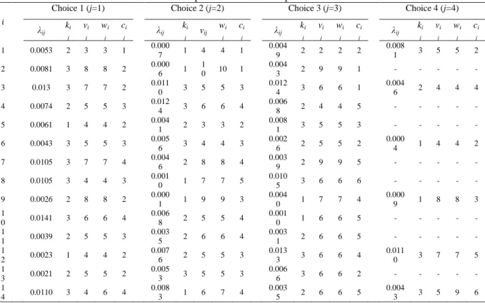
Table 5. Component data for non-repairable section
Choice 1 (j=1) Choice 2 (j=2) Choice 3 (j=3) Choice 4 (j=4)
λij ki j vi j wi j ci
j λij
ki
j vij
wi j
ci
j λij
ki j vi j wi j ci
j λij
ki j vi j wi j ci j
1 0.0053 2 3 3 1 0.0007 1 4 4 1 0.0049 2 2 2 2 0.0081 3 5 5 2 2 0.0081 3 8 8 2 0.0006 1 10 10 1 0.0043 2 9 9 1 - - - - - 3 0.013 3 7 7 2 0.011
0 3 5 5 3
0.012
4 3 6 6 1
0.004
6 2 4 4 4 4 0.0074 2 5 5 3 0.012
4 3 6 6 4
0.006
8 2 4 4 5 - - - - -
5 0.0061 1 4 4 2 0.004
1 2 3 3 2
0.008
1 3 5 5 3 - - - - -
6 0.0043 3 5 5 3 0.005
6 3 4 4 3
0.002
6 2 5 5 2
0.000
4 1 4 4 2 7 0.0105 3 7 7 4 0.004
6 2 8 8 4
0.003
9 2 9 9 5 - - - - -
8 0.0105 3 4 4 3 0.001
0 1 7 7 5
0.010
5 3 6 6 6 - - - - -
9 0.0026 2 8 8 2 0.000
1 1 9 9 3
0.004
0 1 7 7 4
0.000
9 1 8 8 3 1
0 0.0141 3 6 6 4
0.006
8 2 5 5 4
0.001
0 1 6 6 5 - - - - -
1
1 0.0039 2 5 5 3
0.003
5 2 6 6 4
0.003
1 2 6 6 5 - - - - -
1
2 0.0023 1 4 4 2
0.007
6 2 5 5 3
0.013
3 3 6 6 4
0.011
0 3 7 7 5 1
3 0.0021 2 5 5 2
0.005
3 3 5 5 3
0.006
6 3 6 6 2 - - - - -
1
4 0.0110 3 4 6 4
0.008
3 1 6 7 4
0.003
5 2 6 6 5
0.004
3 3 5 9 6
Table 6. Component data for repairable section
Parameters ́ 1 2 3 4 5 6 7 8 9 10 11
́ 0.0004 0.0004 0.0004 0.0004 0.0004 0.0004 0.0004 0.0004 0.00041 0.00041 0.00041
̅́ 0.0005 0.0005 0.0005 0.0005 0.0005 0.0005 0.0005 0.0005 0.00058 0.00058 0.00058
̿́ 0.0004 0.0004 0.0004 0.0004 0.0004 0.0004 0.0004 0.0004 0.000416 0.000416 0.000416
]́ 2.5 2.5 2.5 2.5 2.5 2.5 2.5 2.6 2.6 2.6 2.4
́ 3 3 3 3 3 3 3 3 3 3 3
́ 4 3 5 6 3.6 7 6 4 3.5 3 4.5
The system considered was comprised of 14 non-repairable (in 3 or 4 types) and 11 repairable components connected in series. Table 5 includes data of failure rate, Erlang distribution parameters, purchasing cost and operational cost, volume, and weight for each non-repairable component. Table 6 indicates data of failure rate, Weibull distribution parameters, and repair and replacement costs for repairable components. In addition, Table 7 presents upper bounds for some problem parameters.
Table 7. Upper bound of parameters
Parameter T M ́ W V !́
Figure5. Obtained results for metrics and objectives by
The example was run 50 times with each algorithm and the results a seen, standard MOFA consumed less time than the other algorithms (Fig. 5 the diversity of solutions (DM) the proposed algorithm (MOF
other methods, also among the Pareto solutions, the lowest cost and highest reliability is in MOF the subject of measures MS, NSGA
responses.
The results of the MOF-DE algorithm are summarized in Table number and type of the redundant components for
( =1+ indicates that a redundant component of the second and fourth type is columns of Table 8 present the selected maintenance policies
repairable section where 0 means no preventive action is required in that period, repair and replacement, respectively
time: , 4 (G‡ 14 and replacement at
30 50 70 90
MOFA MOF-DE NSGA
Time
20 30 40 50
MOFA MOF-DE
NSGA-DM
1750 1765 1780 1795
MOFA MOF-DE NSGA
Cost
Obtained results for metrics and objectives by Standard MOFA, MOF-DE, NSGA
The example was run 50 times with each algorithm and the results are presented in Figure 5. As can be seen, standard MOFA consumed less time than the other algorithms (Fig. 5-a). Regarding the NNS and the diversity of solutions (DM) the proposed algorithm (MOF-DE) has the best performance compared to
among the Pareto solutions, the lowest cost and highest reliability is in MOF
the subject of measures MS, NSGA-II and MOFA Pareto showed more uniform distribution among other DE algorithm are summarized in Table 8. The first four columns represent number and type of the redundant components for the non-repairable section. For example the first row
a redundant component of the second and fourth type is needed
columns of Table 8 present the selected maintenance policies that have been taken at each period here 0 means no preventive action is required in that period,
repair and replacement, respectively. For example, for the first component, repair replacement at , 7, 10 (G‡ 13.
NSGA-II MOPSO
3 5 7 9
MOFA MOF-DE NSGA
NNS
-II MOPSO
0 0.05 0.1 0.15
MOFA MOF-DE NSGA
MS
NSGA-II MOPSO
NSGA-II and MOPSO
re presented in Figure 5. As can be a). Regarding the NNS and DE) has the best performance compared to among the Pareto solutions, the lowest cost and highest reliability is in MOF-DE. On II and MOFA Pareto showed more uniform distribution among other 8. The first four columns represent the For example the first row needed * , 2,4+. The last that have been taken at each period in the here 0 means no preventive action is required in that period, and 1 and 2 indicates repair should be done at
NSGA-II MOPSO
Table 8. Selected maintenance actions and redundancy components obtained from MOF-DE
Non-repairable components Repairable Components
1 2 3 4 ́ t 1 2 3 4 5 6 7 8 9 10 11 12 13 14 15
1 0 1 0 1 1 0 0 0 1 0 0 2 0 0 2 0 0 2 1 0
2 1 1 1 0 2 0 0 0 1 0 2 0 0 1 0 0 2 0 0 2
3 1 1 1 0 3 0 0 2 0 0 1 0 2 0 0 1 0 0 2 0
4 1 0 1 0 4 0 0 0 1 0 0 1 0 0 2 0 2 0 0 1
5 1 0 1 0 5 0 2 2 2 0 0 2 0 0 1 1 1 0 0 1
6 0 0 1 0 6 0 1 0 0 1 0 0 2 0 0 1 0 0 2 1
7 1 1 0 0 7 0 1 0 0 2 2 0 0 1 0 0 2 2 0 0
8 1 0 1 0 8 0 1 0 0 2 0 0 2 0 0 2 0 0 1 0
9 0 1 0 1 9 0 1 0 0 2 0 0 1 0 0 2 0 0 1 0
10 1 0 0 0 10 0 1 1 0 0 2 0 0 1 0 0 1 0 0 1
11 1 0 1 0 11 0 1 2 0 2 1 1 0 0 1 0 0 2 0 0
12 1 1 0 1
13 1 2 1 0
14 0 1 0 1
4- 3- Sensitivity Analysis
In addition to the parameters indicated in table 1, different values of m, equation (10),may also be effective in the MOFA, while in all previous studies m = 2. The parameter m determine the relation between the light intensity at each point and the distance to the light source. If the light source is a point, light intensity decreases in proportion to the inverse square of the distance from the source, this means
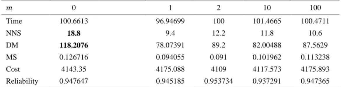
= 2 and if it isanarea light source = 1. These are some facts in the real world; however, in the virtual world they can be dismissed. Thus, by adjusting the values 0, 1, 2, 10and 100for the parameter , the proposed algorithm performance can be reviewed. After running the MOF-DE algorithm20times, the average value of some performance measures was calculated. Table 9 shows the results.
It can be concluded from Table 9 that there is no significant difference for time, MS, and mean value of reliability and cost at different values of parameter ; however, when is equal to zero, NNS and DM are significantly different. This difference can be analyzed when = 0 which indicates the fireflies are not limited to closer brighter ones and results in a wider search space, therefore more Pareto solutions can be found (NNS) and diversity also increases (DM). As other measures show, high diversity does not guarantee the optimal solution with higher quality. Comparison of two other values of m, = 2 showed the better performance of the proposed algorithm
Table 9. Obtained results from different amounts of m by MOF-DE
0 1 2 10 100
Time 100.6613 96.94699 100 101.4665 100.4711
NNS 18.8 9.4 12.2 11.8 10.6
DM 118.2076 78.07391 89.2 82.00488 87.5629
MS 0.126716 0.094055 0.091 0.101962 0.113238
Cost 4143.35 4175.088 4109 4117.573 4175.893
Reliability 0.947647 0.945185 0.953734 0.937291 0.947365
5- Conclusion
In this paper, an effective hybrid approach was used to optimize a reliability problem in a system composed of repairable and repairable components. In this system, two parts of repairable and non-repairable components are connected in series, and to increase the reliability redundant components were used in the first part and preventive maintenance actions were taken in the second part. A problem with the two objectives of increasing overall system reliability and reducing maintenance costs taking into account the constraints of weight, volume and initial budget was formulated. The DE approach was used to develop a standard MOFA and MOF-DE algorithm. The proposed algorithm has benefited from the
advantages of extensive search of the solution space found in DEA and that standard MOFA doesn’t find any new Pareto solution in the iteration of search processes. Numbers of test problems were employed for evaluating the performance of the proposed algorithm with three famous algorithms, standard MOFA, NSGA-II and MOPSO.
Conflict of interests
The authors declare that there is no conflict of interests regarding the publication of this article. References
Amirabadi, H., Khalili, K., Foorginejad, A., & Ashoori, J. (2013). Modeling of abrasive water-jet cutting of glass using artificial neural network and optimization of surface roughness using firefly algorithm. Modares Mechanical Engineering, 13, 123-134.
Azaron, A., Katagiri, H., Kato, K., & Sakawa, M. (2005). Reliability evaluation and optimization of dissimilar-component cold-standby redundant systems. Journal of the Operations Research Society of Japan, 48(1), 71-88.
Chai-ead, N., Aungkulanon, P., & Luangpaiboon, P. (2011). Bees and Firefly Algorithms for Noisy Non-Linear Optimisation Problems. International MultiConference of Engineers and Computer Scientist. Hong Kong.
Chern, M. (1992). On the computational complexity of reliability redundancy allocation in a series system. Operations Research Letters, 11, 309-315.
Coit, D. (2001). Cold-standby redundancy optimization for nonrepairable systems. Iie Transactions,, 33(6), 471-478.
Das, S., & Nagaratnam Suganthan, P. (2011). Differential Evolution: A Survey of the State of the Art. IEEE TRANSACTIONS ON EVOLUTIONARY COMPUTATION, 15, 4-31.
De Castro, H., & Cavalca, K. (2006). Maintenance resources optimization applied to a manufacturing system. Reliability Engineering & System Safety, 91(4), 413-420.
Dieter, A., Pickard, K., & Bertsche, B. (2010). Periodic renewal of spare parts using Weibull. Quality and Reliability Engineering International, 26(3), 193-198.
Dos Santos Coelho, L., de Andrade Bernert, D. L., & Mariani, V. C. (2011). A Chaotic Firefly Algorithm Applied to Reliability-Redundancy Optimization. IEEE Congress on Evolutionary Computation (CEC). New Orleans, LA.
Gandomi, A., Yang, X., & Alavi, A. (2011). Mixed variable structural optimization using Firefly Algorithm. Computers and Structures, 89, 2325-2336.
Garg, H. (2015). An approach for solving constrained reliability-redundancy allocation problems using cuckoo search algorithm. Beni-Suef University Journal of Basic and Applied Sciences, 4(1), 14-25. Goel, N., Gupta, D., & Goel, S. (2013). Performance of Firefly and Bat Algorithm for Unconstrained Optimization Problems. International Journal of Advanced Research in Computer Science and Software Engineering, 31, 1405-1409.
He, Q., Hu, X., Ren, H., & Zhang, H. (2015). A novel artificial fish swarm algorithm for solving large-scale reliability–redundancy application problem. ISA transactions, 59, 105-113.
Heungseob, K., & Pansoo, K. (2017). Reliability models for a nonrepairable system with heterogeneous components having a phase-type time-to-failure distribution. Reliability models for a nonrepairable system with heteroReliability Engineering & System Safety, 37-46.
Huang, H.-Z., Qu, J., & Zuo, M. J. (2009). Genetic-algorithm-based optimal apportionment of reliability and redundancy under multiple objective. IIE Transactions, 41, 287–298.
Jardine, A., & Buzacott, J. (1985). Equipment reliability and maintenance. European Journal of Operational Research, 19(3), 285-296.
Khalili-Damghani, K., Abtahi, A.-R., & Tavana, M. (2013). A new multi-objective particle swarm optimization method for solving reliability redundancy allocation problems. Reliability Engineering & System Safety, 111, 58-75.
Kumar, R., Izui, K., Yoshimura, M., & Nishiwaki, S. (2009). Multi-objective hierarchical genetic algorithms for multilevel redundancy allocation optimization. Reliability Engineering and System Safety, 94, 891-904.
Li, H., & Ye, C. (2012). Firefly Algorithm on Multi-Objective Optimization of Production Scheduling System. Advances in Mechanical Engineering and its Applications, 3, 258-262.
Li, Z., Liao, H., & Coit, D. (2009). A two-stage approach for multi-objective decision making with applications to system reliability optimization. Reliability Engineering and System Safety, 94, 1585-1592. Liang, Y.-C., & Lo, M.-H. (2010). Multi-objective redundancy allocation optimization using a variable neighborhood search algorithm. Journal of Heuristics, 16, 511–535.
Marichelvam, M., Prabaharan, T., & Yang, X. (2014). A Discrete Firefly Algorithm for the Multi-objective Hybrid Flowshop Scheduling Problems. IEEE TRANSCATIONS ON EVOLUTIONARY COMPUTATION, 18, 301 - 305.
MohammadZadeh Dogahe, S., & Sadjadi, S. (2015). A New Biobjective Model to Optimize Integrated Redundancy Allocation and Reliability-Centered Maintenance Problems in a System Using Metaheuristics. Mathematical Problems in Engineering.
Najafi, A., Akhavan Niaki, S., & Shahsavar, M. (2009). A parameter-tuned genetic algorithm for the resource investment problem with discounted cash flows and generalized precedence relations. Computers &OperationsResearch, 36, 2994-3001.
Rebaiaia, M. L., Ait-Kadi, D., Rahimi, S. A., & Jamshidi, A. (2016). Numerical comparative analysis between age and block maintenance strategies in the presence of probability distributions with increasing failure rate. International Federation of Automatic Control, (pp. 1904-1909).
Rigdon, S. (2008). Reliability Optimization. In Encyclopedia of Statistics in Quality and Reliability (pp. 1599-1604). John Wiley & Sons.
Ruiz-Vanoye, J., & Díaz-Parra, O. (2011). Similarities between meta-heuristics algorithms and the science of life. Central European Journal of Operations Research, 19, 445-66.
Safari, J. (2012). Multi-objective reliability optimization of series-parallel systems with a choice of redundancy strategies. Reliability Engineering & System Safety, 108, 10-20.
Salmasnia, A., Ameri, E., & Niaki, S. (2016). A robust loss function approach for a multi-objective redundancy allocation problem. Applied Mathematical Modelling, 40(1), 635-645.
Sayadi, M., Hafezalkotob, A., & Jalali Naini, S. (2013). Firefly-inspired algorithm for discrete optimization problems: An application to manufacturing cell formation. Journal of Manufacturing Systems, 32, 78-84.
Soltani, R., Safari, J., & Sadjadi, S. (2015). Robust counterpart optimization for the redundancy allocation problem in series-parallel systems with component mixing under uncertainty. Applied Mathematics and Computation, 80-88.
Suman, B. (2003). Simulated annealing-based multiobjective algorithms and their application for system reliability. Engineering Optimization, 35, 391–416.
Taboadaa, H., Baheranwalaa, F., & Coit, D. (2007). Practical solutions for multi-objective optimization: An application to system reliability design problems. Reliability Engineering and System Safety, 92, 314-322.
Weibull, W. (1951). A Statistical Distribution Function of Wide Applicability. Journal of applied mechanics.
Yang, X. (2010). Nature-inspired metaheuristic algorithm. Luniver Press.
Yang, X. (2013). Multiobjective Firefly Algorithm for Continuous Optimization. Engineering with Computers, 29, 175-184.
Yang, X.-S., & He, X. (2013). Firefly Algorithm: Recent Advances and Applications. Journal of Swarm Intelligence, 1, 36-50.
Yu, X., & Gen, M. (2010). Introduction to evolutionary algorithms. Springer.
Zhao, J.-H., Liu, Z., & Dao, M.-T. (2007). Reliability optimization using multiobjective ant colony system approaches. Reliability Engineering and System Safety, 92, 109-120.
Zoulfaghari, H., Hamadani, A., & Abouei Ardakan, M. (2014). Bi-objective redundancy allocation problem for a system with mixed repairable and non-repairable components. ISA Transactions, 53, 17-24.