C A S E S T U D Y
Open Access
Relay performance verification using fault
event records
Swagata Das
1, Sundaravaradan Navalpakkam Ananthan
2*and Surya Santoso
2Abstract
Introduction: Event reports recorded by intelligent electronic devices (IEDs) such as digital relays and fault recorders during disturbances depict the status and system parameters of the power system. Incorrect relay settings and unknown system parameters can lead to relay misoperation but information regarding these are available by performing a comprehensive analysis of fault records. Hence, it is necessary to regularly make a comprehensive assessment of the functioning of the relay to ensure reliable operation.
Case description: The objective of this paper is to demonstrate various aspects of evaluating relay performance and verifying circuit parameters which are used in relay settings using field data in two case studies.
Discussion and Evaluation: While scrutinizing the relay’s operation, this paper also presents key insights on verifying circuit parameters using the same relay event records.
Conclusions: The lessons learned from the case studies presented in this paper will equip a protection engineer to inspect the operation of a relay during a transmission line fault, help gain a better understanding of the fault event and take possible actions to prevent future occurrence of similar events.
Keywords: Event report, Fault analysis, Relay
1 Introduction
Relays are vital devices present in any power system. They protect various components in the power system from catastrophic damage during faults. They help in maintaining safe and reliable operation of the entire sys-tem. A recent study analyzing protection system misop-erations was performed by North Electric Reliability Corporation (NERC) and they identified various causes for relay misoperations [1]. All these emphasize the need to make comprehensive assessment of relay operation and its performance regularly.
Event reporting is a very useful feature in intelli-gent electronic devices (IEDs) such as digital relays and fault recorders. Event reports contain voltage and cur-rent waveforms which depict the fault characteristics at the time of occurrence. They are traditionally used for fault analysis such as fault classification and identify-ing the fault location but contain much more additional
*Correspondence:[email protected]
2Department of Electrical and Computer Engineering, The University of Texas at Austin, Austin, USA
Full list of author information is available at the end of the article
information which can be used to improve the power system reliability.
System operators usually have detailed circuit mod-els of transmission and distribution networks in CAPE [2], OpenDSS [3], and other power system software [4]. The circuit model is useful for conducting short-circuit studies, determining protective relay settings, and choos-ing the maximum ratchoos-ing of circuit breakers and other power system equipment. Incorrect short-circuit model parameters can lead to erroneous relay settings and relay misoperations, an example of which is described in [5]. As a result, it is essential that the circuit parameters are accu-rately known and the system model is continually updated to reflect any system additions, repairs, or modifications.
Several authors in the past have attempted to glean additional information from fault records [6–10]. Using event reports, authors in [11,12] have estimated the zero-sequence line impedance of a two-terminal line. Similarly, the authors of [8] have calculated the Thevenin impedance of the system upstream from the measured location using event reports. The authors of [13] have further explored in detail about deriving zero-sequence line impedance using data from both the terminals of a two-terminal line as well
as using data from only one end of the line. These high-light the presence of plethora of information in an event report and the need for comprehensive analysis of event reports.
Based on the above background, the objective of this paper is to use relay event reports to comprehensively evaluate the relay performance and circuit parameters which are used in relay settings instead of just one or two parameters such as those presented in [8–13]. The con-tribution of this paper lies in demonstrating the above by analyzing two case studies in detail. The following appli-cations of IED data for above purpose are presented in this paper: (a) relay and circuit breaker performance eval-uation, (b) event reconstruction, (c) zero-sequence line impedance validation, (d) detection of incorrect power system equipment installation, (e) fault resistance and root-cause identification, and (f ) circuit model verifica-tion. It presents the theory of potential applications of IED data to improve power system reliability. Each section consists of description of the fault incident, the current and voltage waveforms associated with it followed by the analysis.
2 Case study 1: B-G fault verifies relay
performance, validates the zero-sequence line impedance, and authenticates the system model
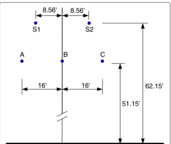
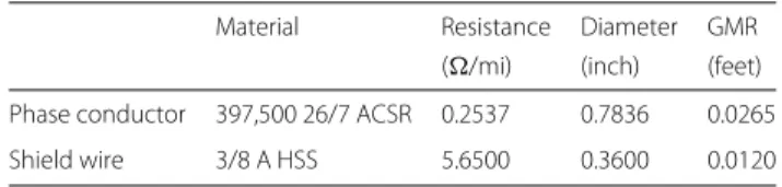
In this case study, the circuit model of the utility trans-mission network was available in CAPE software [2] as shown in Fig.1. The rated voltage at Substation A is 161 kV. A relay is responsible for protecting the 23.6-mile long transmission line that connects Substation A with Sub-station C. The line geometry is shown in Fig.2 and the conductor data are provided in Table1. This line data is used in Carson’s equations to calculate the positive- and zero-sequence line impedances as ZL1=6.01 +j19.00 andZL0=19.72 +j56.23, respectively.
A single line-to-ground fault on phase B occurred at a distance of 14.37 miles from Substation A as illustrated
Fig. 2Overhead transmission line spacing (in feet)
in Fig. 1. The root cause of the fault is not known. The fault, being momentary in nature, is cleared by the first shot of the relay. However, the same fault reappears in the circuit after 15 minutes as seen from the event log in Fig. 3. The relay operates again to allow the temporary fault to clear from the circuit. During the entire duration, the relay records four 16-cycle long events, whose voltage and current waveforms are shown in Fig.5.
In the following subsections, the waveform data is used to reconstruct the sequence of events, estimate the fault location, estimate the fault resistance, validate the zero-sequence line impedance, and verify the accuracy of the system model and demonstrate what we can learn from these about the relay performance and operation.
2.1 System protection description
The settings of the relay are shown in Fig.4. The relay is programmed to perform three automatic reclosures. The
Table 1Conductor data
Material Resistance Diameter GMR (/mi) (inch) (feet)
Phase conductor 397,500 26/7 ACSR 0.2537 0.7836 0.0265
Shield wire 3/8 A HSS 5.6500 0.3600 0.0120
first reclose open interval (79IO1) is 10 cycles, the sec-ond reclose open interval (79I02) is 1800 cycles, and the third reclose open interval (79IO3) is 3600 cycles. The relay resets itself when the fault disappears from the trans-mission feeder for more than 900 cycles. A trip occurs when the phase instantaneous element with directional control (67P1T), the phase time-overcurrent (51PT) ele-ment, the ground instantaneous element with directional control (67G1T), or the ground time-overcurrent (51NT) element asserts as evident from the TR equation in Fig.4. Now, 67P1T asserts when the phase current is greater than 1048.80 A primary and the relay trips with no inten-tional time delay. On the other hand, if the phase current is between 540 A primary and 1048.80 A primary, the phase time-overcurrent pickup element, 51P, picks up and starts to time on the U3 curve whose equation is given as:
t=TD×
0.0963+ 3.88 M2−1
(1)
wheretis the relay trip time in seconds,Mis a multiple of pickup and is calculated as the ratio of the fault current to the pickup setting, andTDis the time dial setting. When 51P times out, 51T asserts and causes the relay to initiate a trip.
During a ground fault, if the relay detects a ground current greater than 560.40 A primary, element 67G1T asserts and the relay trips instantaneously. When the ground current is greater than 288 A primary but less than 560.40 A primary, the ground time-overcurrent pickup element, 51G, asserts and starts timing on the U3 curve. Once 51G times out, 51GT asserts and trips
Fig. 3Case study 1: Relay fault event history
Fig. 4Case study 1: Settings in the relay
the relay. It is important to note that 67P1T and 67G1T are disabled for shot 1 as specified by the trip equation in Fig.4. Logical operator ‘!’ indicates a NOT function, operator ‘*’ indicates a AND function, operator ‘/’ indi-cates a rising edge trigger, and SH1=1 when the relay is at shot=1. In other words, during shot 1, the relay will trip only for 51PT and 51GT elements.
2.2 Event report trigger criteria
The digital relay records an event report under two con-ditions: (a) when the TR equations asserts and the relay trips or (b) when the ER equation asserts. The ER equation consists of the phase and ground time-overcurrent ele-ments, 51P and 51G, as shown in Fig.4. When either of 51P or 51G or the TR equation is asserted, the ER equation asserts and the digital relay records an event report.
2.3 Event reconstruction
a
b
c
d
Fig. 5Events recorded by the relay.aEvent 4 voltage and current waveforms at shot = 0.bEvent 3 voltage and current waveforms at shot = 1. cEvent 2 voltage and current waveforms at shot = 0.dEvent 1 voltage and current waveforms at shot = 1
When 79OI1 times out, the circuit breaker closes back into the circuit at 12:44:38.885 hours as shown by Event 3 in Fig.5b, and the shot counter increases to 1. The fault, however, is still present in the circuit and the relay mea-sures a phase and ground current of 2860 A and 2811 A, respectively. Since the operation of the 67P1T and 67G1T elements are suspended in shot 1, the ground time-overcurrent element picks up at 12:44:38.893 hours and starts timing on the U3 curve. The phase time-overcurrent element also picks up at 12:44:38.897 hours and triggers this event. According to (1), the operating time of the phase and ground time-overcurrent elements are 0.316 and 0.203 secs, respectively. As a result, 51GT asserts before 51P has a chance to time out and issues a trip signal to the circuit breaker. Because the relay records only 16 cycles of waveform data, the opening of the circuit breaker is not shown.
By the time the relay starts recording Event 2 at 12:59:41.476 hours, the circuit breaker has already closed back into the circuit. The fault has cleared and the phase B current has returned back to normal load current lev-els as shown in Fig.5c. The relay has also reset itself since the fault was absent from the transmission network for more than 900 cycles. Unfortunately, the fault reappears on phase B at 12:59:41.526 hours. Element 67G1T asserts immediately and trips the circuit breaker. The relay starts timing on the first open interval, 79OI1.
When 79OI1 times out, the circuit breaker closes back into the circuit, and the shot counter increases to 1. The fault, however, persists, and the relay measures a phase
and a ground current of 3380 A and 3340 A, respectively. Since the operation of the 67P1T and 67G1T elements are suspended for shot 1, both the phase and the ground time-overcurrent elements pick up at 12:59:41.995 h and start timing on the U3 curve. The more sensitive ground time-overcurrent, 51GT, times out before its phase counterpart, 51PT, and trips the circuit breaker at 12:59:42.186 h. No other event reports were provided. Therefore, it is not clear whether this shot of the relay removed the fault or whether the relay eventually locked out to isolate the permanent fault.
2.4 Relay performance assessment
In the previous subsections, we have reviewed the relay settings, understood its expected behaviors and recon-structed the sequence of events. This subsection aims to assess the performance of the relay and to determine whether relay operating times are within set time limits. The approach for this is by comparing the expected time of operation with the actual relay operating time. When calculating the expected operating time of the relay, the functional specifications of the relay must be taken into consideration.
2.4.1 Assessment of Trip Time during the Shot 1 in Event 3
Fig. 6Case study 1: Functional specifications of the relay
The relay has a pickup accuracy of ±3% of setting
±0.05 A. Therefore, for a pickup setting of 2.40 A sec-ondary, the pickup accuracy equals±0.122 A. This means that when the actual fault current is 23.425 A secondary, 51G can assert when the current is between 23.303 A and 23.547 A secondary (23.425±0.122 A).
Suppose the relay picks up at 23.303 A secondary (M=9.71). Using (1), the operating time of the relay is 0.2040 secs. As per Fig.6, 51P has a curve timing accu-racy of±4% of the operating time and±1.5 cycle. For an operate time of 0.2040 secs, the curve timing accuracy equals 0.0331 secs (4%×0.2040 + 0.025 secs). Therefore, the relay is expected to operate within 0.1709 and 0.2372 secs (t1= 0.2040±0.0331 secs).
Alternatively, suppose the relay picks up when the fault current is 23.547 A secondary (M=9.81). From (1), the operating time of the relay is solved to be 0.2028 secs. The curve timing accuracy for this operate time is calcu-lated to be 0.0331 secs (4%×0.2028 + 0.025 secs). There-fore, the relay will operate within 0.1697 and 0.236 secs (t2=0.2028±0.0331 secs).
The final time window, tfinal, that accounts for both
pickup and curve timing accuracy can be calculated as Min (t2)<tfinal<Max (t1) or 0.1697<tfinal<0.2372
secs. Therefore,the relay is expected to operate within 0.1697 and 0.2372 secs. From Fig. 5b, 51GP asserts at 12:44:38.897 hours while 51GT asserts at 12:44:39.072 hours. Therefore, the actual operating time of 0.175 secs falls within the expected window of operation and hence, the relay performs as expected.
2.4.2 Assessment of trip time during the shot 1 in event 1
During shot 1 in Event 1, the relay measures a ground fault current magnitude of 3340 A primary (3340/CTR=27.83 A secondary). Following the proce-dure outlined in Subsection 2.4.1, the relay is expected to operate within 0.1528 and 0.2184 secs. From Fig.5d, 51GP asserts at 12:59:41.995 hours while 51GT asserts at 12:59:42.186 hours. Therefore, the actual operating time of 0.191 secs lies within the expected window of operation and hence, the relay performs as expected.
2.5 Fault location
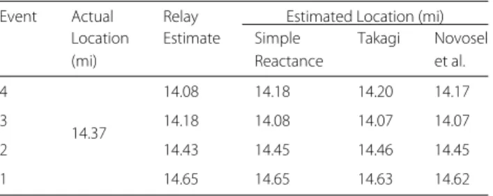
Distance to the fault was computed by applying one-ended fault location algorithms such as the simple reactance,
Takagi, and Novoselet al.methods to all the four events [14]. Notice that Event 4 and Event 2 are short-duration faults with a significant DC offset. Therefore, the third cycle after fault inception was chosen to compute the fault current phasors and minimize any error due to DC off-set. Results tabulated in Table 2 indicate that the fault location estimates from the one-ended algorithms are in good agreement with those estimated by the relay and are close to the actual fault location. The relay’s estimated fault location and the manually calculated fault location using various algorithms matching the actual location of the fault helps us indirectly verify that: (a) the currents recorded by the relay match the actual currents seen at the input of the relays without any errors in the settings of instrument transformers (b) the system parameters have been accurately programmed into the relay.
2.6 Fault resistance estimation
Using voltage and current waveforms from one end of the line and the known fault location, Eriksson and Novosel et al. algorithms [15,16] can be used to estimate the fault resistance as
RF =
d−mb
f (2)
The form taken by constantsb,d, andf depends on the fault type and the number of terminals in a transmission line as defined for the Novosel et al. algorithm in [14] and mis the distance to the fault. As seen from Table3, the fault resistance is expected to lie between 0.02 and 1.7. The knowledge of fault resistance helps in short circuit model verification which is shown in Section2.9.
2.7 Thevenin Impedance estimation
Since Events 4 through 1 describe an unbalanced fault with a return path to the ground, the waveforms cap-tured in those events can be used to estimate the positive-, negative-, and zero-sequence Thevenin impedances upstream from the relay. The negative-, zero- and positive-sequence Thevenin impedance was calculated using (3), (4) and (5). The estimated Thevenin impedances
Table 2Case study 1: Location estimates from one-ended methods
Event Actual Relay Estimated Location (mi) Location Estimate Simple Takagi Novosel
(mi) Reactance et al.
4
14.37
14.08 14.18 14.20 14.17
3 14.18 14.08 14.07 14.07
2 14.43 14.45 14.46 14.45
Table 3Case study 1: Estimated values of fault resistance
Event Fault resistance ()
4 0.02
3 0.06
2 0.90
1 1.70
were then compared with the circuit model in CAPE to gauge the accuracy of estimation.
ZG2= − VG2
IG2
(3)
ZG0= − VG0
IG0
(4)
ZG1= − VG
IG = −
VG1−VG1pre
IG1−IG1pre
(5)
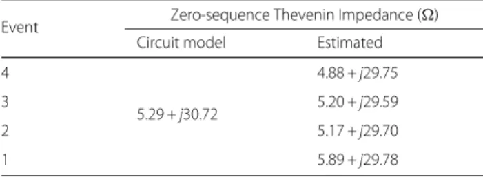
As seen in Tables 4 and 5, the reactance component of the Thevenin impedances are a good fit with those obtained from the circuit model. The resistive component, on the other hand, show greater variations. Perhaps the resistance is affected by the temperature increase in con-ductors and transformer windings due to fault currents.
2.8 Zero-sequence line impedance validation
Since the fault described in Events 4 through 1 involve a return path through the ground, it is possible to use the event data captured by the relay to verify the zero-sequence line impedance. The zero-sequence line impedance was calculated using (6) and the results are shown in Table6. The magnitude and phase angle errors were calculated using (7).
ZL0=
VG−mZL1(IG1+IG2) mIG0
(6)
Magnitude Error%
= ||Actual Z|L0| − |Estimated ZL0||
Actual ZL0| ×
100
Phase Angle Error
= |∠Actual ZL0−∠Estimated ZL0| (7)
Table 4Case study 1: Actual vs. estimated positive- and negative-sequence Thevenin impedances
Event
Positive-sequence Negative-sequence
Impedance () Impedance ()
Circuit model Estimated Circuit model Estimated
4
2.82 +j17.90
3.62 +j17.35
2.91 +j18.03
2.94 +j17.09
3 1.90 +j18.36 3.18 +j16.84
2 4.12 +j17.31 3.13 +j17.08
1 1.43 +j18.77 3.71 +j17.11
Table 5Case study 1: Actual vs. estimated zero-sequence Thevenin impedance
Event Zero-sequence Thevenin Impedance () Circuit model Estimated
4
5.29 +j30.72
4.88 +j29.75
3 5.20 +j29.59
2 5.17 +j29.70
1 5.89 +j29.78
From Table 6, it can be concluded that the estimated zero-sequence line impedance matched well with that computed using Carson’s equations at an earth resistivity value of 100m. This helps in verifying the zero-sequence line impedance setting of the relay as they play an impor-tant role in distance and directional protection.
2.9 Short-circuit model verification
Event reports captured by the recloser can be used to confirm the accuracy of the circuit model in CAPE. The approach is to replicate the actual fault in the circuit model and compare the resulting short-circuit current with actual field measurements. As an example, Event 1 was recreated by simulating a B-G fault in the CAPE cir-cuit model at the known location of the fault, i.e., 14.37 miles from the substation as shown in Fig. 1. The fault resistance estimated in Table 3, RF=0.02, was used.
Comparison between the short-circuit current in CAPE and the fault current measured by the relay in Event 1 is shown in Fig. 7. The currents match well once the DC offset decays out after the third cycle. Comparison between short-circuit currents in CAPE and relay mea-surements for all the remaining events are presented in Table7. Matching relay measurement currents and simu-lated short-circuit currents in CAPE show that the input contacts of the relay are working fine and there are no errors in the settings of the instrument transformers in the relay. Furthermore, results presented in Table7 indi-cate that the circuit model in CAPE is representative of the actual transmission network and this can be used to verify the relay settings.
Table 6Case study 1: Actual vs. estimated zero-sequence line impedance
Event
Zero-sequence line Impedance () Error
Carson’s equation Estimated Magnitude Phase angle (%) (degrees)
4
19.72+j56.22
24.06+j55.03 0.79 4.29
3 23.60+j54.30 0.63 4.16
2 21.84+j56.75 2.05 1.72
Fig. 7Fault current in the circuit model matches well with that measured by the relay in Event 1
2.10 Lessons Learned
Successful analysis of this event verified the performance of the relay. In addition, the event report was used to vali-date the zero-sequence line impedance setting in the relay. Furthermore, the fault record was used to estimate the fault resistance and Thevenin impedance which helped to gain further knowledge about the fault as well as assist in short circuit model verification. Calculating the fault loca-tion and simulating fault scenarios similar to those in the event reports verified that there were no errors in settings of the instrument transformers, the input contacts were working fine and the circuit model is representative of the actual transmission network. The reason why several methods have been presented to verify various relay set-tings and relay operation is because it may not be possible to implement all of the above verification steps in every fault scenario.
3 Case study 2: Lightning strike on a 161-kV
transmission line reveals incorrect CT polarity and missing phase CT
A 161-kV transmission line experienced a three-phase fault due to a lightning strike at 5.86 miles from Station
Table 7Short-circuit current in CAPE vs. actual measurements from the relay
Event Actual location Estimated location Fault current (kA)
(mi) (mi) Relay CAPE
4
14.37
14.18 2.36 2.19
3 14.08 2.30 2.19
2 14.45 2.34 2.18
1 14.65 2.33 2.17
VG,IG
Station 1 Fault Point F VH,IH Station 2
5.86 mi 17.53 mi
DFR DFR
ZG1 ZH1
Fig. 8Case study 2 is a ABC fault at 5.86 miles from Station 1 or 17.53 miles from Station 2
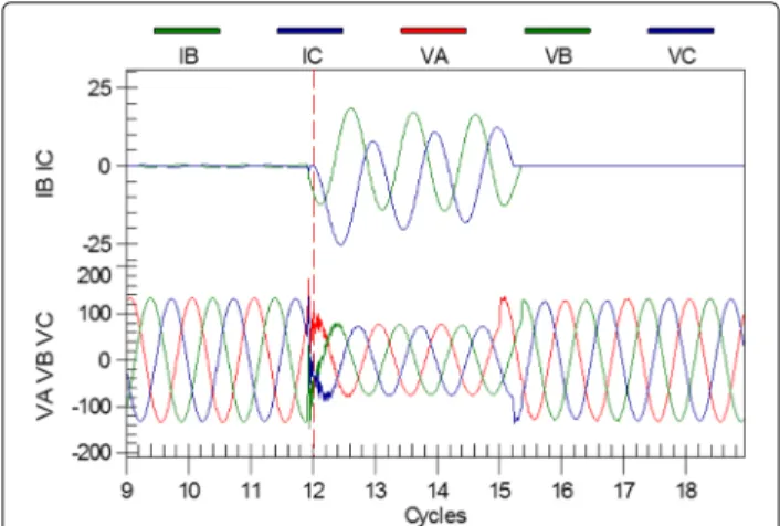
1 or 17.53 miles from Station 2 as shown in Fig. 8. The transmission line is 23.39 miles long and has a positive-and zero-sequence impedance of ZL1=2.85+j18.22 andZL0=16.80+j60.89, respectively. A Digital Fault Recorder (DFR) at Station 1 captures the voltage and cur-rent waveforms at 100 samples per cycle as shown in Fig.9. Notice that the phase A current waveform is miss-ing. The prefault current at Station 1 is 150 A while the fault current is 11 kA. The three-phase voltage and cur-rent waveforms at Station 2 are recorded by a DFR having a sampling rate of 96 samples per cycle and are shown in Fig.10. The prefault current is 200 A while the fault current magnitude is 3.6 kA.
3.1 Fault location
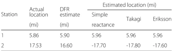
When one-ended fault-locating algorithms are applied to Station 1 data, distance-to-fault estimates are close to the actual location of the fault as seen in Table8. Estimates from one-ended algorithms applied to Station 2 data are also close to the actual fault location. However, it is puz-zling to observe that the distance estimates are negative. Most likely, the CT has been installed with a reverse polar-ity and hence, measures current in a direction opposite to the fault as illustrated in Fig.11. The reverse CT polar-ity is further evident if one looks closely at the positive-and negative peak of the voltage positive-and current waveforms recorded at Station 2. As shown in Fig.10, when current in
Fig. 10Case study 2: Voltage and current waveforms at Station 2
a particular phase has a positive peak, the corresponding voltage has a negative peak, i.e., a 180-degree phase shift. Therefore, the negative location estimate can be inter-preted as 17.80 miles upstream with respect to the Station 2 DFR direction shown in Fig. 11. It is also interesting to observe that the DFR at Station 2 underestimated the fault location by a mile. It is possible that the incorrect CT polarity or inaccurate line parameters contributed to the fault location error.
Because the sampling rate of the DFRs at Station 1 and Station 2 are not equal, the unsynchronized two-ended method [14] was chosen to estimate the fault location. The missing phase A current at Station 1 did not allow for the calculation of sequence components. However, since the event is a balanced three-phase fault, it was possible to use phase components instead of symmetrical compo-nents. The reverse polarity of the CT at Station 2 was also taken into account. The fault location estimated by this method was 5.71 miles from Station 1 which is close to the actual fault location. Since fixing the reverse polarity of the CT at Station 2 got us a fault location estimate close to the actual fault location, it verifies that it was the source of error for negative fault location initially.
3.2 Thevenin Impedance estimation
Since the fault event is a balanced three-phase fault, only the positive-sequence Thevenin impedance could be esti-mated from the fault data using (5) as shown in Table9. Results indicate that Station 2 is electrically weaker than
Table 8Location estimates from one-ended methods
Station Actual DFR
Estimated location (mi)
location estimate Simple
Takagi Eriksson
(mi) (mi) reactance
1 5.86 5.90 5.96 5.96 5.96
2 17.53 16.60 -17.70 -17.80 -17.60
VG,IG
Station 1 Fault Point F VH,IH Station 2
5.86 mi 17.53 mi
DFR DFR
ZG1 ZH1
Fig. 11Negative distance estimate from Station 2 indicates that the meter direction is reversed
Station 1. Although the circuit model is not available, judging from the fault currents contributed by each sta-tion, impedance estimates are likely to be accurate.
3.3 Lessons learned
Analysis of fault data can reveal incorrect setup of power system equipment or incorrect field wiring that was missed during field commissioning tests. Results of the analysis can be used to take corrective action and avoid future misoperations. For example, this event shows that the CT at Station 2 was installed with an incorrect polarity. As a result, the direction of the current was reversed and can affect the reliability and performance of directional relays. Furthermore, the phase A current measurement at Station 1 was missing. It is possible that the phase CT has not been connected to the DFR and can result in loss of valuable information. The fault was observed to have encountered the least resistance path to the ground, which coincides with the root cause of the fault. Finally, Station 2 was learned to be electrically weaker than Station 1.
4 Conclusion
This paper uses field data collected from utility transmis-sion and distribution networks to demonstrate a variety of methods to analyze various aspects of relay operation from different angles. The following contribute to relay operation and relay settings assessment:
• Relay and Circuit Breaker Performance Evaluation
IEDs record what they “see” during a fault and those records can be used to assess the performance of relays and circuit breakers. For example, Case study 1 con-firmed that the relay performed as expected during that fault event. If the protective relay had operated slower than expected during the fault, the utility can carefully monitor the future trip operations of this relay to ensure that the relay is not out of tolerance.
Table 9Estimated positive-sequence source impedances
Station Source Impedance ()
1 0.46 +j3.66
• Validating the Zero-sequence Line Impedance Single line-to-ground or double line-to-ground fault events can be used to validate the zero-sequence impedance of the transmission line as shown in Case study 1.
• Estimating the Fault Resistance
Fault data captured at one or both ends of the line can be used to estimate the fault resistance. Interpretation of this value is useful in determining the root cause of the fault. Knowing the fault resistance value also plays a significant role while verifying the accuracy of the short-circuit model as demonstrated in Case study 1.
• Estimating the Thevenin Impedances
Estimating the Thevenin impedance during a fault helps in validating the short-circuit model and can also provides valuable feedback about the state of the transmission network upstream from the monitoring location.
• Estimating the Fault Location
Apart from being able to accurately locate the fault so as to quickly clear it, a lot more information about the relay can be derived from estimating the fault location using different methods such as identifying errors in instrument transformer connections and settings, and verifying that the system parameters have been accu-rately programmed into the relay as shown in Case study 1. Since fault location uses a lot of parameters in its calculation, it helps verify all the factors and variables which influence it.
• Verifying the accuracy of the system short-circuit
model used for simulation studies
Event reports help not only in confirming the accu-racy of the short-circuit model but by comparing simulated short-circuit currents and relay measured currents it can help locate errors in input contacts and connections as well as identify errors in instrument transformer settings in the relay. Furthermore, it can help validate all the circuit parameters that have been programmed into the relay.
• Detecting incorrect installation of power system
equipment
Analysis of fault data can reveal incorrect setup of power system equipment or incorrect field wiring that was missed during field commissioning tests. Results of the analysis can be used to take corrective action and avoid future misoperations. For example, Case study 2 detects a CT with incorrect polarity and a digital fault recorder with a missing measurement channel.
Amongst the numerous parameters that can be calcu-lated from relay event reports, estimation of some of these parameters can be automated and used instantly whereas the estimation of other parameters requires them to be
done offline with manual procedures to obtain maximum benefits.
Relay and circuit breaker performance evaluation can be automated and performed every time a fault has occurred. This can serve as a continuous supervision of the relay and circuit breaker operation. Most digital relays have fault location algorithms embedded in them which can approximate the fault location as soon as it records an event report.
Though the process of estimating the fault resistance can be automated, it is not commonly implemented in a digital relay. It requires the attention of a protection engineer (PE) to estimate the fault resistance and inter-pret it. Similarly, the process of estimating the Thevenin impedance, zero-sequence line impedance and other short-circuit model parameters requires a PE to be able to study the system, validate the calculated values and make use of them. Likewise, detecting incorrect installation of power system equipment also requires the skills of a PE.
Authors’ contributions
SD had performed the analysis using relay event reports. SNA assisted in performing the analysis and drafting the manuscript. SS was the technical advisor and supervised the analysis and submission of the manuscript. All authors read and approved the manuscript.
Competing interests
The authors declare that they have no competing interests.
Author details
1Schweitzer Engineering Laboratories, Pullman, USA.2Department of Electrical
and Computer Engineering, The University of Texas at Austin, Austin, USA.
Received: 1 February 2018 Accepted: 31 May 2018
References
1. Bian, JJ, Slone, AD, Tatro, PJ (2014). Protection system misoperation analysis, In2014 IEEE PES General Meeting | Conference & Exposition, National Harbor, MD(pp. 1–5).
2. (1999).CAPE User’s Programming Language Reference Manual: Electrocon International Inc.
3. Dugan, RC (2013).The Open Distribution System Simulator (OpenDSS) Ref. Guide. Palo Alto: Electric Power Research Institute.
4. Bam, L, & Jewell, W (2005). Review: power system analysis software tools, In IEEE Power Engineering Society General Meeting, 2005. Vol. 1 (pp. 139–144). 5. (2010).Lesson Learned: Short-Circuit Models (Relay Settings and Equipment
Specifications). https://www.nerc.com/pa/rrm/ea/Lessons Learned Document Library/LL20100502 Short Circuit Models (Relay Settings and Equipment Specifications).pdf.
6. Costello, D (2008). Lessons learned analyzing transmission faults, In2008, 61st Annual Conference for Protective Relay Engineers(pp. 410–422). 7. Das, S, & Santoso, S (2016). Utilizing relay event reports to identify settings
error and avoid relay misoperations, In2016 IEEE/PES Transmission and Distribution Conference and Exposition (T&D), Dallas, TX(pp. 1–5). 8. Sharma, C, & Castellanos, F (2006). Remote fault estimation and thevenin
impedance calculation from relays event reports, In2006 IEEE/PES Transmission & Distribution Conference and Exposition: Latin America (pp. 1–7).
9. Henville, CF (1998). Digital relay reports verify power system models.IEEE Transactions on Power Delivery,13(2), 386–393.
11. Amberg, A, Rangel, A, Smelich, G (2012). Validating transmission line impedances using known event data, In65th Annual Conference for Protective Relay Engineers(pp. 269–280).
12. Schweitzer, III EO (1990). A review of impedance-based fault locating experience, In14th Annual Iowa-Nebraska System Protectection Seminar (pp. 269–280).
13. Das, S, Ananthan, SN, Santoso, S (2017). Estimating zero-sequence line impedance and fault resistance using relay data.IEEE Transactions on Smart Grid.
14. Das, S, Santoso, S, Gaikwad, A, Patel, M (2014). Impedance-based fault location in transmission networks: theory and application.IEEE Access,2, 537–557.
15. Eriksson, L, Saha, MM, Rockefeller, GD (1985). An accurate fault locator with compensation for apparent reactance in the fault resistance resulting from remote-end infeed.IEEE Trans. Power App. Syst,PAS-104(2), 423–436. 16. Novosel, D, Hart, D, Hu, Y, Myllymaki, J (1998). System for locating faults