Available online throug
ISSN 2229 – 5046
ON SINGLE TERM HAAR WAVELET SERIES METHOD
FOR VOLTERRA INTEGRO-DIFFERENTIAL EQUATIONS
S. Sekar*
Department of Mathematics, Government Arts College (Autonomous),
Salem-636 007, Tamil Nadu, India
C. Jaisankar
Department of Mathematics, A.V.C. College (Autonomous),
Mannampandal, Mayiladuthurai – 609 305, Tamil Nadu, India.
(Received on: 07-03-14; Revised & Accepted on: 18-03-14)
ABSTRACT
I
n this paper present a reliable algorithm for solving Volterra Integro-Differential Equations (VIDE) using single-term Haar wavelet series (STHWS) method. The obtained discrete results were compared with exact solution of the VIDE and methods taken from the literature [1, 4] to highlight the efficiency of the STHWS method. Some illustrative examples have been presented to illustrate the implementation of the algorithm and efficiency of the method.Mathematics Subject Classification: 41A45, 41A46, 41A58.
Keywords:Haar wavelet; single-term Haar wavelet series (STHWS), Integro-Differential Equations, Volterra
Integro-Differential Equations.
1. INTRODUCTION
Mathematical modelling of real-life problems usually results in functional equations, e.g. partial differential equations, integral and integro-differential equation, stochastic equations and others. Many mathematical formulations of physical phenomena contain integro-differential equations, these equations arise in fluid dynamics, biological models and chemical kinetics. Integro-differential equations are usually difficult to solve analytically so it is required to obtain an efficient approximate solution. Several numerical methods for approximating the Fredholm or Volterra integro-differential equations are known.
A number of problems in chemistry, physics and engineering are modelled in terms of system of Volterra integro-differential equations. Various methods have been developed to prove existence and uniqueness of solutions to integro-differential equations [2, 5 – 6, 15 - 17]. In this paper, we use a Single-Term Haar Wavelet Series (STHWS) method for solving the Volterra integro-differential equations. This method was first presented by S. Sekar and team of his researchers [3, 7 – 13, 14] for solving IDE and Fredholm IDE of the second Kind, Analysis of the Fuzzy IDE, A study on linear and nonlinear stiff problems and fuzzy differential equations, Nth-order fuzzy differential equations, Hybrid fuzzy systems, A study on second-order fuzzy differential equations and to solve one dimensional fuzzy differential inclusions. Recently, the authors have used Homotopy Perturbation Method (HPM) [1] and the Block Pulse Functions (BPF) and their operational matrices [4] method for the numerical solution of Volterra integro-differential equations to prove their efficiency.
In this article we developed numerical methods for VIDEs to get discrete solutions via STHWS method which was studied by S. Sekar and team of his researchers [7 - 13]. The paper is organized as follows: In section 2, we describe Haar wavelet series, their properties and STHWS methods. In section 4, general format for VIDEs discussed. Finally in section 5 we apply the proposed method on some examples which was taken from the literature [1,7] to show the accuracy and efficiency of the STHWS method.
Corresponding author: S. Sekar*
2. PROPERTIES OF HAAR WAVELET AND STHW TECHNIQUE
2.1 HAAR WAVELET SERIES
The orthogonalset of Haar wavelets
h
i( )
t
is a group of square waves with magnitude of±
1
in some intervals and zeros elsewhere. In general,h
( )
t
h
1(
2
t
k
)
,
j
n
=
−
Wheren
k
j
+
=
2
,j
≥
0
,
0
≤
k
<
2
j,
n
,
j
,
k
∈
Z
.
Any function y(t), which is square integrable in the interval [0, 1) can be expanded in a Haar series with an infinite number of terms
,
)
(
)
(
0∑
∞ ==
i i ih
t
c
t
y
Wherei
=
2
j+
k
(1)
where the Haar coefficients
j
≥
0
,
0
≤
k
<
2
j,
t
∈
[
0
,
1
)
,
=
∫
( )
1
0
)
(
2
y
t
h
t
dt
c
i j i are determined such that thefollowing integral square error
ε
is minimized∫
( )
∑
( )
−
=
− = 1 0 2 1 0,
dt
t
h
c
t
y
m i i iε
Wherem
=
2
j,
j
∈
{ }
0
∪
N
Furthermore
,
,
0
2
0
,
0
,
2
,
2
2
)
(
)
(
1 0 1
≠
<
≤
≥
+
=
=
=
=
− −∫
h
t
h
t
dt
i
i
l
l
k
j
k
j jj il
j
i
δ
usually, the series expansionEq. (1) contains an infinite number of terms for a smooth y (t). If y (t) is a piecewise constant or may be approximated as a piecewise constant, then the sum in Eq. (1) will be terminated after m terms, that is
( ) ( )
[
)
10
( )
( )
( ),
0,1
m
T i i m m i
y t
c h t
c
h
t
t
=
=
≈
∑
=
∈
( )
( )
[
0 1...
1]
,
T m m
t
c
c
c
c
=
−( )
[
( ) ( )
( )
]
Tm m
t
h
t
h
t
h
t
h
=
0,
0,...,
−1where “T” indicates transposition, the subscript m in the parentheses denotes their dimensions,
C
( )Tmh
(m)(
t
)
denotes the truncated sum. Since the differentiation of Haar wavelets results in generalized functions, which in any case should be avoided, the integration of Haar wavelets are preferred.
Integration of Haar Wavelets should be expandable in Haar series
∫
∑
∞ =
=
t i i i md
C
h
t
h
0 0
)
(
)
(
τ
τ
If we truncate ton
m
=
2
terms and use the above vector notation, then integration is performed by matrix vector multiplication and expandable formula into Haar series with Haar coefficient matrix defined by [7].( )
( )
( ) ( )[
)
10
( ),
0,1
m m m m
h
τ τ
d
≈
E
×h
t
t
∈
∫
where the m-square matrix E is called the operational matrix of integration which satisfies the following recursive equations ( )
−
=
× − × × × × 2 2 1 2 2 2 2 2 20
2
1
2
1
m m m m m m m m m mH
m
H
m
E
E
(2)( )
−
=
×0
4
1
4
1
2
1
2 2E
and ( )2
1
1 1×
=
The
[
]
m
i
x
m
i
x
h
x
h
x
h
x
h
H
m×m=
n(
0),
n(
1).
n(
2)...,
m(
m−1)
,
≤
i≤
+
1
( )
1
( )(
),
1r
dia
H
m
H
−m×m
Tm×m
=
1,1, 2, 2, 4, 4, 4,...
,
,
...
,
2
2 2 2
2
T
n
m m m
m
r
m
=
>
Proof of equation (2) is found in [5]. Since
H
(mxm)andH
(−m1×m)contain many zeros. Let us define( )
( )
t
h
( )(
t
)
M
( )(
t
)
h
m Tm≈
m×m , andM
( )1×1(
t
)
=
h
0(
t
)
satisfyingM
(m×m)(
t
)
c
( )m=
C
(m×m) ( )h
m(
t
)
andC
( )1×1=
c
0.2.2 SINGLE TERM HAAR WAVELET SERIES TECHNIQUE
With the STHWS approach, in the first interval, the given function is expanded as STHWS in the normalized interval
τ
∈
[ )
0
,
1
, which corresponds to
∈
m
1
,
0
τ
by definingτ
=
mt
, m being any integer. In STHWS, thematrix becomes
2
1
=
E
. Let( )
•
τ
x
andx
( )
τ
be expanded by STHWS in the first interval asx
( )
τ
=
ν
( )1h
o( )
τ
•
,
( )
τ
( )( )
τ
0 1h
x
x
=
and in the nth interval as,x
( )
τ
=
ν
( )nh
o( )
τ
•
,
x
( )
τ
=
x
( )nh
0( )
τ
Integrating (9) with
1
2
E
=
, we get ( ) ( )( )
0
2
1
1 1x
x
=
ν
+
. Wherex
(0)
is the initial condition. According to [7],we have ( )1
=
∫
x
( )
d
=
x
( ) ( )
1
−
x
0
•
τ
τ
ν
In general, for any interval n, n=1, 2...
We obtain, ( ) ( )
(
1
)
2
1
+
−
=
v
x
n
x
n n (3)x
( )
n
=
v
( )n+
x
(
n
−
1
)
(4)Equation (3) and (4) give the discrete time values of
x
( )n andx
( )
n
x n
( )
for the nth interval. These values from the basis for the estimating block pulse values and discrete values in the subsequent normalized time intervals.3. VOLTERRA INTEGRO-DIFFERENTIAL EQUATIONS
Consider the general form of linear Volterra integro-differential equation is of the form [1,4]
( ) ( ) ( )
( )
( ) ( )
( )
=
≤
≤
+
=
+
′
∫
0
,
,
y
a
y
b
x
a
dt
t
y
t
x
k
x
f
x
y
x
x
y
xa
λ
µ
Where the functions f (x), μ (x) and the kernel k(x,t) are given functions, whereas y(x) needs to be determined.
4. NUMERICAL EXAMPLE
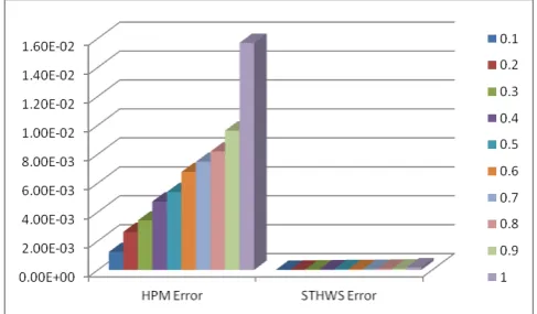
time = 0.1) along with exact solutions of the examples 1 to 4 and absolute errors between them are calculated and are presented in Table 1 to 4. A graphical representation is given for the VIDEs in Figures 1 to 4, using three-dimensional effect to highlight the efficiency of the STHWS method.
Example: 1 Consider the linear Volterra integro-differential equation [1]
( ) ( )
(
)
( )
( )
=
≤
≤
−
+
+
+
+
=
+
′
−∫
10
0
1
0
,
8
5
1
2
0 2
2
y
x
dt
t
ty
x
e
x
x
x
y
x
y
x xFor which the exact solution is
y
( )
x
=
10
−
xe
−x.Example: 2 Consider the linear Volterra integro-differential equation [1]
( ) ( )
( )( )
( )
=
≤
≤
=
+
′
∫
−1
0
1
0
,
0
y
x
dt
t
y
e
x
y
x
y
x t xFor which the exact solution is
y
( )
x
=
e
−xcosh
x
.Example: 3 Consider the linear Volterra integro-differential equation [4]
( )
( )
( )
=
=
′
∫
1
0
,
0
y
dt
t
y
x
y
xFor which the exact solution is
y
( )
x
=
cosh
x
. Indeed, in this example, we havef
( )
x
=
0
,µ
( ) ( )
x
y
x
=
0
and( )
,
=
1
=
k
x
t
λ
Example: 4 Consider the linear Volterra integro-differential equation [4]
( )
( )
( )
=
−
=
′
∫
0
0
,
1
0
y
dt
t
y
x
y
x
For which the exact solution is
y
( )
x
=
sin
x
. Indeed, in this example, we haveλ
=
f
( )
x
=
1
,µ
( ) ( )
x
y
x
=
0
and( )
x
,
t
=
−
1
k
Figure 1. Error estimation of Example 1
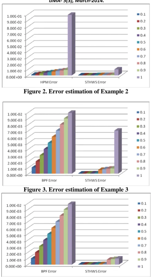
Figure 2. Error estimation of Example 2
Figure 3. Error estimation of Example 3
Figure 4. Error estimation of Example 4
5. CONCLUSIONS
In this paper, we have successfully approximated the solution of the form (1) of Volterra integro-differential equations. To this end, we have used STHWS methods. Moreover, the error of the proposed method is analyzed. For more investigation, some examples have been presented. As the numerical results showed, the proposed method is an effective method to solve the Volterra integro-differential equations. The benefit of the method is simplicity for execution and using Haar series which make the method cheap as computational costs.
Table 1: Exact Solutions and Error calculation of Example 1
x
Example 1 Exact
Solutions
HPM Error
Table 2: Exact Solutions and Error calculation of Example 2
x
Example 2 Exact
Solutions
HPM Error
STHWS Error 0.1 1.110701379 1.00E-03 1.00E-05 0.2 1.245912349 2.00E-03 2.00E-05 0.3 1.4110594 3.00E-03 3.00E-05 0.4 1.612770464 4.00E-03 4.00E-05 0.5 1.859140914 5.00E-03 5.00E-04 0.6 2.160058461 6.00E-03 6.00E-04 0.7 2.527599983 7.00E-03 7.00E-04 0.8 2.976516212 8.00E-03 8.00E-04 0.9 3.524823732 9.00E-03 9.00E-04 1.0 4.194528049 9.90E-02 9.90E-03
Table 3: Exact Solutions and Error calculation of Example 3
x
Example 3 Exact
Solutions
BPF Error
STHWS Error 0.1 1.005004168 1.00E-03 1.00E-06 0.2 1.020066756 2.00E-03 2.00E-06 0.3 1.045338514 3.00E-03 3.00E-05 0.4 1.081072372 4.00E-03 4.00E-05 0.5 1.127625965 5.00E-03 5.00E-05 0.6 1.185465218 6.00E-03 6.00E-04 0.7 1.255169006 7.00E-03 7.00E-04 0.8 1.337434946 8.00E-03 8.00E-04 0.9 1.433086385 9.00E-03 8.50E-04 1.0 1.543080635 9.90E-03 7.00E-03
Table 4: Exact Solutions and Error calculation of Example 4
x
Example 4 Exact Solutions
BPF Error
STHWS Error 0.1 0.099833417 1.00E-03 1.00E-07 0.2 0.198669331 2.00E-03 2.00E-06 0.3 0.295520207 3.00E-03 3.00E-06 0.4 0.389418342 4.00E-03 4.00E-06 0.5 0.479425539 5.00E-03 5.00E-05 0.6 0.564642473 6.00E-03 6.00E-05 0.7 0.644217687 7.00E-03 7.00E-05 0.8 0.717356091 8.00E-03 8.00E-04 0.9 0.78332691 9.00E-03 9.00E-04 1.0 0.841470985 9.90E-03 9.90E-04
REFERENCES
[1] Behrouz Raftari, “Numerical Solutions of the Linear Volterra Integro-differential Equations: Homotopy Perturbation Method and Finite Difference Method”, World Applied Sciences Journal, Vol. 9, 2010, pp. 07-12. [2] S. M. El-Sayed and M. R. Abdel-Aziz, “Comparison of Adomians decomposition method and wavelet-Galerkin method for solving integro-differential equations”. Appl. Math. Comput., Vol. 136, 2003, pp. 151–159.
[3] C. Jaisankar, S. Senthilkumar and S. Sekar, “Numerical Solution for Fredholm Integro Differential Equations of the second Kind via Single-Term Haar Wavelet Series Method”, European Journal of Scientific Research, Vol. 96, Issue 1, February, 2013, pp. 38-42.
[5] R. C. MacCamy, “An integro-differential equation with application in heat flow”, Quart. Appl. Math., Vol. 35, 1977, pp. 1–19.
[6] E. Paramanathan and S. Sekar, “An Application of STHW Technique in Solving Non-linear Integro-Differential Equations”, Journal of Applied Sciences Research, Vol. 8, Issue 9, 2012, pp. 4815-4820.
[7] S. Sekar and C. Jaisankar, “Numerical Solution for the Integro-Differential Equations using Single Term Haar Wavelet Series Technique”, International Journal of Mathematical Archive, Vol. 4, Issue 11, 2013, pp. 97-103. [8] S. Sekar and C. Jaisankar, “Numerical Analysis of the Fuzzy Integro-Differential Equations using Single-Term Haar Wavelet Series”, International Journal of Mathematics Trends and Technology, Vol. 5, Issue 1, 2014, pp. 168-175.
[9] S. Sekar and E. Paramanathan, “A Study on Linear and Nonlinear Stiff Problems Using Single-Term Haar Wavelet Series Technique”, International Journal of Mathematical Analysis, Vol. 7, Issue 53, 2013, pp. 2625-2636. [10] S. Sekar and S. Senthilkumar, “Single Term Haar Wavelet Series for Fuzzy Differential Equations”, International Journal of Mathematics Trends and Technology, Vol. 4, Issue 9, 2013, pp. 181-188.
[11] S. Sekar and S. Senthilkumar, “Numerical Solution of Nth-Order Fuzzy Differential Equations by STHWS Method”, International Journal of Scientific & Engineering Research, Vol. 4, Issue 11, November-2013, pp. 1639-1644.
[12] S. Sekar and S. Senthilkumar “Numerical Solution for Hybrid Fuzzy Systems by Single Term Haar Wavelet Series Technique”, International Journal of Mathematical Archive, Vol. 4, Issue 11, 2013, pp. 23-29.
[13] S. Sekar and S. Senthilkumar, “A Study on Second-Order Fuzzy Differential Equations using STHWS Method”, International Journal of Scientific & Engineering Research, Vol. 5, Issue 1, January-2014, pp. 2111-2114. [14] S. Senthilkumar, C. Jaisankar and S. Sekar, “Comparison of Single Term Haar Wavelet Series Technique and Euler method to Solve One Dimensional Fuzzy Differential Inclusions”, Journal of Applied Sciences Research, Vol. 9, Issue 9, 2013, pp. 73-79.
[15] Shishen Xie, “Numerical Algorithms for Solving a Type of Nonlinear Integro-Differential Equations”, World Academy of Science, Engineering and Technology, Vol. 41, 2010, pp. 1083-1086
[16] N.H. Sweilam, “Fourth order integro-differential equations using variational iteration method”, Comp.Math. Appl., doi:10.1016/j.camwa.2006.12.055
[17] B. Neta, “Numerical solution of a nonlinear integro-differential equation”, J. Math. Anal. and Appl., Vol. 89, 1982, pp. 598–611.