Optimizing Sort in Hadoop using
Replacement Selection
by
Pedro Martins Dusso
A thesis submitted in partial fulfillment for the degree of Master of Science
in the
Fachbereich Informatik
AG Datenbanken und Informationssysteme
I, Pedro Martins Dusso, declare that this thesis titled, ‘Optimizing Sort in Hadoop using Replacement Selection’ and the work presented in it are my own. I confirm that:
This work was done wholly or mainly while in candidature for a research degree at this University.
Where any part of this thesis has previously been submitted for a degree or any other qualification at this University or any other institution, this has been clearly stated.
Where I have consulted the published work of others, this is always clearly at-tributed.
Where I have quoted from the work of others, the source is always given. With the exception of such quotations, this thesis is entirely my own work.
I have acknowledged all main sources of help.
Where the thesis is based on work done by myself jointly with others, I have made clear exactly what was done by others and what I have contributed myself.
Signed:
Date:
Abstract
Fachbereich Informatik
AG Datenbanken und Informationssysteme
Master of Science
by Pedro Martins Dusso
This thesis implements and evaluates an alternative sorting component for Hadoop based on the replacement-selection algorithm. Hadoop is an open source implementation of the MapReduce framework. MapReduce’s popularity arises from the fact that it provides distribution transparency, linear scalability, and fault tolerance. This work proposes an alternative to the existing load-sort-store solution which can generate a small number of longer runs, resulting in a faster merge phase. The replacement selection algorithm usually produces runs that are larger than available memory, which in turn reduces the overall sorting time. This thesis first describes different sorting algorithms for in-memory sorting and external sorting; secondly, it describes Hadoop and Hadoop’s map tasks and output buffer strategies; thirdly, it describes four sorting implementation alternatives, which are presented from the most simple to the most complex. Furthermore, this work analyzes the performance of these four alternatives in terms of execution time for run generation and merging, and the number of intermediate files produced. Finally, we provide a critical analysis with respect to Hadoop’s default implementation.
and work — a great environment filled with marvelous and intelligent people. Professor H¨arder’s career and work are a huge inspiration for me, and I can only hope to cause a small portion of the great impact that his work has caused in our science and in our society. The foundations are laid, now it’s our turn. I would also like to offer my special thanks to my advisor, colleague, tutor, friend, roommate, sports and drinking partner Caetano Sauer. I have learn from him philosophy, linguistics, politics, astronomy, math-ematics, photography, history, and also a little of computer science. We probably have not “solved out” all of our problems, but I’m sure we have much harder questions to answer today than when we met. My special thanks are extended to V´ıtor Uwe Reus, a friend which I do not hesitate to call a brother, and who has shared with me not only our work space but also many trains and bottles. I believe the sayings in the beginning of this paragraph are true, because merely walking next to these men made myself a much better individual.
My most beloved thanks goes to Carolina Ferret, who filled with love and care not only our first house here in Germany but my life as a whole. Her endeavor coming with me while I as pursuing this title was a huge love act, and which I will always be thankful to. Traveling, eating, listening to music, dancing, and all the best things in life are even better when we can share them with someone we love and I share with her. I will never be able to be grateful enough to my family, which never get tired of asking when I was coming back. To my mother, Cl´audia, for her infinite patience and infinite strength. To my father, Eduardo, for the clear path to follow. To my brother, Henrique, for being so different to me but so similar at same time. For all friends I made during this journey,
Ich hoffe wir auf den Straßen der Welt treffen.
Declaration of Authorship i
Abstract iii
Acknowledgements iv
List of Figures vii
List of Tables ix 1 Introduction 1 1.1 Motivation . . . 1 1.2 Contribution . . . 2 2 Sorting 4 2.1 In-memory sorting . . . 4 2.1.1 Quicksort . . . 6 2.1.2 Heapsort . . . 7 2.1.3 Mergesort . . . 8
2.2 External memory sorting. . . 9
2.2.1 Run generation with quicksort . . . 11
2.2.2 Run generation with Replacement Selection . . . 12
2.2.3 Comparison . . . 13
2.2.4 Merge . . . 14
3 Hadoop 18 3.1 Motivation . . . 18
3.2 Running a MapReduce job. . . 19
3.3 Map and Reduce tasks . . . 20
3.3.1 The Map Side. . . 22
3.4 Pluggable Sort . . . 28
4 Implementation 31 4.1 Development and experiment environment . . . 31
4.2 Record Heap . . . 32 v
4.4 Prefix Pointer Heap . . . 43
4.5 Prefix Pointer with Custom Heap . . . 44
5 Experiments 48 5.1 Asynchronous Writer . . . 48
5.1.1 Single disk . . . 49
5.1.2 Dual disks. . . 50
5.2 Ordered, Partially Ordered and Reverse Ordered . . . 51
5.3 Real World Jobs . . . 58
6 Conclusions 60
2.1 Quicksort procedure . . . 6
2.2 Array and equivalent complete binary tree . . . 8
2.3 Heapsort procedure . . . 9
2.4 Mergesort procedure . . . 10
2.5 Multiway merge with four runs . . . 14
2.6 Four-way merging . . . 15
2.7 Multiway merge with four runs with buffer . . . 16
2.8 Merging twelve runs into one with merging factor of six . . . 17
3.1 How Hadoop runs a MapReduce job . . . 20
3.2 Map and reduce tasks in detail . . . 21
3.3 In-memory buffers: key-value and metadata . . . 24
3.4 Kvoffsets buffer sorted by partition . . . 25
3.5 Two spill files and the resulting segments for each partition . . . 27
3.6 Merge tree with 20 segments and merge factor 10 . . . 28
3.7 The map task execution . . . 29
4.1 Testing setup of micro-benchmarks . . . 32
4.2 Comparison between Hadoop’s MapOutputBuffer and our custom RecordHeap buffer . . . 34
4.3 Java’s heap space in two different scenarios . . . 35
4.4 A possible state of a memory buffer with its corresponded memory manager 38 4.5 Flowchart describing the collection method of PointerHeap . . . 39
4.6 Flowchart describing the flushing method of PointerHeap . . . 40
4.7 Comparison between Hadoop’s MapOutputBuffer and our custom PointerHeapbuffer. . . 40
4.8 Fragmentation levels depending on the input data . . . 42
4.9 Comparison between Hadoop’s MapOutputBuffer and our custom PointerHeapbuffer. . . 43
4.10 Percentage of comparisons decided with key prefix and full key for random strings and English words . . . 44
4.11 MetadataHeap fields . . . 45
4.12 Comparison between all output buffers . . . 46
4.13 Comparison betweenPrefixPointerHeap and PPCustomHeap . . . 47
4.14 Comparison betweenPrefixPointerHeap and PrefixPointerCustomHeap 47 5.1 The circular buffer and the writer thread . . . 49
5.2 Run generation with a single disk or dual disks . . . 50
5.6 Lineitem table sorted by orderkey column . . . 53
5.7 Partially ordered file by shipdate results . . . 54
5.8 Partially ordered file by receiptdate results . . . 54
5.9 Lineitem table sorted by second date column . . . 55
5.10 Number of records in the buffer and number of free blocks . . . 56
5.11 Number of occupied blocks . . . 57
5.12 Length of raw records and rounded records from lineitem table . . . 57
5.13 Join of lineitem and order tables, using a buffer size of 100MB . . . 58
2.1 Comparison of Storage Technologies . . . 10 2.2 Run generation with replacement selection . . . 12 4.1 Sample from EnglishWords and RandomStrings input files. . . 41
Introduction
1.1
Motivation
It has being a decade since the first papers about the so called MapReduce framework were published [1–3] by Google. During this period, data management research on big data moved from the laboratories to the reality of working clusters with thousands of machines, where a volume of data in the order of petabytes is processed daily running some implementation of the MapReduce framework. Most of this popularity can be credited to MapReduce’s open source version, called Hadoop, released by Yahoo! and today supported by the Apache Foundation. Hadoop runs on commodity hardware, making it easy and cheap to deploy; it provides both a programming model and a soft-ware framework for analysis of distributed datasets, which frees the developers (or, using a modern term, the data scientists) from the technical aspects of distributed execution over a cluster, fault tolerance, process communication, and data sharing, letting them focus on the analytical algorithms needed to solve the existing problems.
During the last years, Hadoop is evolving thanks to the contribution of its users — which are not only persons but also companies like Cloudera, Yahoo, Facebook, IBM, and others. Nevertheless, there is a lot of room for improvement in two main landscapes: the first is the development of additional tools that enhance the abstraction of the framework in different levels and integrate it with other data management tools. In [4], J. Kobielus anticipates that massively parallel data processing systems will not make traditional warehousing architectures obsolete; instead, they will supplement and extend the data warehouse in strategic roles such as extract/transform/load (ETL), data staging, and preprocessing of unstructured content. Working in this direction, the data management community can achieve an integrated (but diverse) platform for multi-structured data.
challenges for developers of extensions and customizations. Changes are slow, and many of the new features are implemented by third-party entities (a customization due a particular necessity) and integrated into the main branch. This highly heterogeneous and decoupled development environment makes the code hard to understand and modify, which was one of the main challenges in this thesis. Hadoop was first released in 2007 and in 2012 its second (alpha) version became public, with major features such as federation of the underlying distributed file system, a dedicated resource negotiator, and many performance improvements.
1.2
Contribution
This thesis implements and evaluates an alternative sorting component for Hadoop based on the replacement-selection algorithm [7]. Sorting is used in Hadoop to group the map outputs by key and deliver them to the reduce function. The original implementation is based on quicksort, which is simple to implement and very efficient in terms of RAM and CPU. However, data management research has shown that replacement selection may deliver higher I/O performance for large datasets [8,9]. Sorting performance is critical in MapReduce, because it is essentially the only non-parallelizable part of the computation. The sort stage of a MapReduce job is very network- and disk-intensive, and thus the superiority of quicksort for in-memory processing may not be directly manifested in this scenario. Our goal in this thesis is to evaluate replacement selection for sorting inside Hadoop jobs. To the best of our knowledge, this is the first approach in that direction, both in academia and in the open-source community.
The remainder of this thesis is organized as follows. Chapter 2 reviews algorithms for in-memory and disk-based sorting, focusing on the replacement-selection algorithm. In chapter3, we present the internals of job execution in Hadoop, focusing on the algorithms and data structures used to implement external sorting using quicksort. The infrastruc-ture presented will serve as basis for our implementation of replacement selection, which will be discussed in Chapter 4. We implemented four versions of the algorithm using different mechanisms for internal memory management and sort processing. Our goal was to start from a simple naive implementation and gradually improve it to deliver the best possible performance. An experimental evaluation of each alternative in compar-ison with Hadoop’s original method is also presented. In Chapter 5, we compare our
replacement-selection method against original Hadoop, using a wide range of scenarios representative of real-world usage. The experiments in this chapter are executed at the level of whole MapReduce jobs, instead of the micro-benchmarks performed in Chapter 4. Finally, chapter 6 concludes this thesis, providing a brief overview of the pros and cons of our solution, as well as discussing numerous open challenges for future research.
Sort algorithms can be classified into two main categories. When the input data set fits in main memory, an internal sort can be executed. If not, an external sort algorithm is needed. We sort in-memory using sorting algorithms such as quicksort, heapsort, mergesort, and others.
It is necessary to rethink the sorting procedure when the input data set is bigger than the available main memory. Memory devices slower than the computer main memory (e.g., hard disk) must work together to bring the records in the desired ordering. The combination of sorting input subsets in memory followed by an external merge process is the basic recipe of an external sorting algorithm.
A record is a basic unit for grouping and handling data. It can represent one single integer number or a more complex data structure, such as a personal address book composed by name, telephone number and address fields. A key is a special field (or subset of fields) used as criterion for the sort order. A value is the data associated to a specific key, i.e., the rest of the record. Whether key and value are disjoint or one is a subset of the other is irrelevant for our discussion.
2.1
In-memory sorting
In-memory sorting algorithms present different strategies and consequently different complexities, which in turn influence their efficiency. When deciding which in-memory sorting algorithm to use we consider the number of records in the input: for less than one hundred records any algorithm is equally efficient because the input is too small; but when dealing with a number of records between one hundred and the maximum number of records that still fit in main memory anO(nlog(n)) algorithm is preferrable
[10]. Before discussing the three mainO(nlog(n)) sorting algorithms (namely quicksort, heapsort, and mergesort) we introduce some concepts to classify these algorithms. This categorization will help us later to decide which algorithm to use.
Astable sort is a sort algorithm which preserves the input order of equal elements in the sorted output; i.e., if whenever there are two recordsr andswith the same key and with
r appearing beforesin the original list,r will appear befores in the final sorted output. An in-place algorithm is an algorithm which transforms input using a data structure with a constant amount of extra storage space. The input is usually overwritten by the output as the algorithm executes.
We can further classify sorting algorithms with respect to its general operational method. These methods are:
1. Insertion: when examining record j assume all previously records 1. . . j−1 are already sorted. Then, move the actual record to the correct position, shifting higher ranked records up as necessary.
2. Exchanging: systematically interchange pairs of records that are out-of-order until no more such pairs exist.
3. Selection: repeatedly select the smallest (or biggest) record from the input. One by one we move the selected record to an output data structure, until the input is empty.
4. Merging: combine two or more sorted inputs into a single ordered one.
5. Distribution: records are distributed from their input to multiple intermediate structures which are then gathered and placed on the output.
The first algorithm we discuss is quicksort, which is an unstable, in-place, and exchanging sort. Perhaps quicksort is the most used sort algorithm in general, given that it is the algorithm used in the Microsoft .NET Framework [11] and in Oracle Java 7 [12]. Furthermore, it is the sort algorithm used by the Hadoop MapReduce framework. We also discuss heapsort, an unstable, in-place, selection sort, because its selective strategy backed by a heap will be useful when we talk about replacement selection. Finally, we introduce mergesort, a stable, non-in-place, merging sort. Its sort strategy based on merging sorted inputs is used in external sorting algorithms, thus reviewing the mergesort algorithm provides a good background to work on in the next section. A comprehensive study of sorting algorithms and techniques is found in [7].
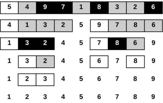
Figure 2.1: Quicksort procedure: white boxes represent the current pivot; grey boxes represent the records smaller than the pivot and the black boxes the records bigger than the pivot. Records outside any box are already in their final ordered position.
2.1.1 Quicksort
Quicksort is an exchanging sort algorithm that, on average, makes O(nlog(n)) compar-isons to sort n records. It has a O(n2) complexity in the worst case, but it is usually faster than other O(nlog(n)) algorithms in practice [10]. Furthermore, quicksort’s se-quential and localized memory references exhibit superior address locality, which allows exploiting processor caching [13]. Quicksort implementations are usually unstable, but stable versions exist [14].
Quicksort work as follows: given an input ofn records, we take a recordr (calledpivot) and move it to the final position p it should occupy in the output. To determine p, we rearrange the other records so that all records with a key value greater than that of r are “to the right” of p (i.e., their positions are greater that p) and the rest to the left. At this point, we havepartitioned the input into two smaller sets: the set of values smaller thanr, and the set of values greater thanr. Now the original sorting problem is reduced to these two smaller problems, namely sorting the two smaller partitions. This is a typical application of the divide and conquer strategy, and we show an example in Figure 2.1. The algorithm is applied recursively to each subset, until all records are in their final position.
2.1.2 Heapsort
The heapsort algorithm is based on the heap data structure. The heap is usually placed in an array with the layout of a complete binary tree, which is “a binary tree in which every level, except possibly the deepest, is completely filled; at depth n, the height of the tree, all nodes must be as far left as possible” [15]. The binary tree structure is mapped to array indices: for a zero-based array, the root of the tree is stored at index 0. The left and right children of a node in position i are given by 2i+ 1 and 2i+ 2, respectively. Similarly, the parent of i is found b(i−1)/2c. During the construction of the heap structure, the data in the array is in an arbitrary ordered. The positions are then rearranged to preserve the heap property: the key of a node i is greater (or less) than or equal to that of its children. To restore the property, theheapify operation is invoked to rearrange the array elements. The heapify process can be thought of as building a heap from the bottom up, successively shifting nodes downward to establish the heap property. More details in building the heap structure are found in [7] and [10]. In Figure2.2 we show a heap (constructed over an array) and its corresponding binary tree.
If we can transform an input set into a heap, we can sort the input simply by always selecting the root element for output until the heap is empty. This makes heapsort a selection-based algorithm. Differently from quicksort, heapsort has an O(nlog(n)) average case complexity, regardless of the order of the input dataset. However, it is slower than a tuned quicksort in practice [10].
The algorithm is divided into two parts: first, a heap is built out of the input data; and second, a sorted array is built by repeatedly removing the largest (or the smallest) record from the heap and inserting it into the sorted output. After each removal, the heap is reconstructed, i.e., a heapify is invoked.
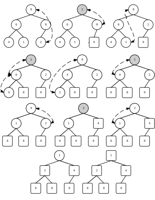
Once all records from the input are inserted into the heap, we can start selecting the largest record. This record at the root of the tree is swapped with the last leaf node, which is located at the end of the array. The array is then heapified again, excluding the last position of the array. This process is repeated for all records in the heap until only the root node remains in the tree. At this point, the records are sorted. This process is illustrated in Figure 2.3, where circle nodes represent records to be sorted, square nodes represent already sorted records, shaded nodes represent the start of a new heapify operation, and finally dashed arrows represent a shift operation (used during the heapify process to rearrange the nodes to keep the heap property).
Figure 2.2: Array and equivalent complete binary tree
2.1.3 Mergesort
Mergesort is a merging-based sort algorithm where most implementations are stable, differently from quicksort. Mergesort has an average and worst-case performance of
θ(nlog(n)), however it demands θ(n) auxiliary space. In-place versions also exist but,
due to the constant factors involved, they are only of theoretical interest [16].
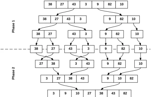
Mergesort has two phases: first, we divide the unsorted input set into n subsets of size 1, which are obviously sorted. Second, we combine two or more ordered subsets into a single ordered one. This is called the merge phase. In the second step, we repeatedly compare the smallest remaining record from one subset with the smallest remaining record from the other input subset. The smallest of these two (assuming a two-way
merge, where only two subsets are merged at a time) records is moved to the output. The process repeats until one of the subsets becomes empty. Figure 2.4 shows both of these steps. The output of a merge step can be an intermediary output, which will be further merged with other intermediary outputs or a final output, when all n subsets divided into the first step have been merged into one last sorted set of size n.
We can cover many possible sorting scenarios with these three sorting algorithms in our tool set. When auxiliary space is not an issue and we desire a tight upper bound for our worst case complexity, we shall use mergesort. When we need to sort in-place or we have knowledge about the unsorted input to explore cache locality, we shall use the quicksort. Heapsort will be of special interest when we detail the replacement selection algorithm
Figure 2.3: Heapsort procedure
in the following section, because it borrows the heap and the selection strategy from heapsort.
2.2
External memory sorting
We useexternal sort when the input dataset does not fit in the available main memory. From now on, we should use the terms disk, hard disk, and external memory indistinctly. The same is valid for memory, main memory, and internal memory. Nowadays, hard disks are the most common form of external memory device. If we compare them to main memory, hard disks present the following properties, as seen in [17]:
Figure 2.4: Mergesort procedure first dividing the input until subsets of size 1 and then merging the subsets into one single ordered output.
Parameter DRAM NAND Flash Hard Disk PCM
Density 1X 4X N/A 2-4X Read latency (granularity) 20-50ns (64B) ∼25µs (4KB) ∼5ms (512B) ∼50ns (64B) Write latency (granularity) 20-50ns (64B) ∼500µs (4KB) ∼5ms (512B) ∼1µs (64B) Endurance N/A 104 ∼105 ∞ 106 ∼108
Table 2.1: Comparison of Storage Technologies. Adapted from [18].
• The amount of such storage on hard disks often exceeds the amount of main memory by at least two orders of magnitude;
• Hard disks are much slower (up to five orders of magnitude) because they have moving mechanical parts;
• It is beneficial to access more than one item at a time to amortize this time gap between main memory and hard disk.
Often, reading a page from the hard disk takes longer than the time to process it. Thus, CPU instructions stop being the unit to measure cost in the context of external sorting, and we replace it by the number of disk accesses—or I/O operations—performed. This difference makes algorithms designed only to minimize CPU instructions perform not so efficiently when analyzed from the I/O point of view. External memory algorithms must aim to minimize the number of I/O operations. In Table2.1, we see that reading a 4KB page takes∼25µs on flash memory, while reading a 64B page from main memory
takes about 20-50ns. For disk reads, a 512B page takes ∼5ms. For comparison with CPU access speeds, in 5ms an average modern CPU can execute∼105 instructions. Suppose we must sort a file of 5 million records residing on disk, but only 1 million can fit into internal memory at a time. A common solution is to bring each of the five subfiles to main memory, sort it using an internal sort algorithm, and store it back into disk. We call a sorted subfile of records a run. These runs are then merged by reading records of each run sequentially into a merge buffer, in a way that guarantees that the buffer contains at least one record of each run at all times. Once the buffer is full, the smallest record is moved to the output file. This process is repeated until there are no records left in all input runs and the buffer is empty. To allow for fast selection of the smallest record in the buffer, a heap data structure is used.
The above process is similar to the mergesort algorithm, but instead of occurring all at the same time in main memory, the input is consumed in chunks that fit in main memory. For a given input filef of sizesrecords and main memory which accommodates
m records, where s > m, a multiway merging sort can be described in two phases: run generation, where intermediary sorted subfiles, i.e., runs, are produced, andmerge, where multiple runs are merged into a single ordered one. With respect to run generation, two strategies are worth discussing: one using quicksort and another using replacement selection as the in-memory sort algorithm.
2.2.1 Run generation with quicksort
Run generation based on the quicksort algorithm is a simple, nevertheless effective, strategy to create the sorted subfiles. We repeat the following steps until the input file is empty:
1. Read records from f into main memory until the available main-memory buffer is full;
2. Sort the records in main memory using quicksort; 3. Write them into a new temporary file (run).
If we assume fixed-length records such thatm records fit in main memory, this process is repeated ms times, resulting inr := ms runs of sizem stored in the disk.
above). This estimation was first proposed by E.H. Friend in [19] and later described by E.F. Moore in [20], and is also described in [7]. In real world applications, input data is usually not random (i.e., it often exhibits some degree of pre-sortedness). In such cases, the runs generated by replacement selection tend to contain even more than 2m records. In fact, for the best case scenario, namely when the input data is already sorted, replacement selection producesonly one run.
Given a set of tuples hrecord, statusi, where recordis a record read from the unsorted input and status is a Boolean flag indicating whether the record is active or inactive. Active records are candidates for the current run, while inactive records are saved for the next run. The idea behind the algorithm is as follows: assuming a main memory of size m, we read m records from the unsorted input data, setting its status to active. Then, the tuple with the smallest key and active status is selected and moved to an output file. When a tuple is moved to the output (selection), its place is occupied by another tuple from the input data (replacement). If the record recently read is smaller than the one just written, its status is set to inactive, which means it will be written to the next run. Once all tuples are in the inactive state, the current run file is closed, a new output file is created, and the status of all tuples is reset to active.
Step Memory contents Output
1 503 087 512 061 061 2 503 087 512 908 087 3 503 170 512 908 170 4 503 897 512 908 503 5 (275) 897 512 908 512 6 (275) 897 653 908 653 7 (275) 897 (426) 908 897 8 (275) (154) (426) 908 908 9 (275) (154) (426) (509) (end of run) 10 275 154 426 509 154 11 275 612 426 509 275
Table 2.2: Run generation with replacement selection
We introduce another example from [7] in Table 2.2to explain in detail the replacement selection algorithm. Assume an input dataset consisting of twelve records with the following values: 061, 512, 087, 503, 908, 170, 897, 275, 653, 426, 154, 509 and
612. We represent the inactive records in parentheses. A discussion of efficient ways of selecting the smallest record (e.g., using a heap) is postponed to Chapter 4.
In step 1, we load the first four records from the input data into the memory. We select 061 as the smallest then output and replace it for 908. The smallest now is 087, which we move to the output and replace with 170. The just-added record is also the smallest in step 3, so we move it out and replace it with 897. Now we have an interesting situation: when we replace the record 503, the record read from the input is 275, which issmaller
than 503. Thus, since we cannot output 275 in the current run, we set it as inactive—a state which will be kept until the end of the current run. Steps 6, 7, and 8 proceed normally until we move out record 908, which is replaced by 509. At this point, in step 9, all records in memory are inactive. We close the current run, revert the status of all records to active, and continue the algorithm normally.
In this small example, we produce a first run with twice the size of the available memory and a second smaller one. In Table2.2, steps 12, 13, and 14 will output 426, 509, and
612. We calculate this by (tr)modulo(2m) = (12)modulo(2×4) = 5.
2.2.3 Comparison
Replacement selection is a desirable alternative for run generation for two main reasons: first, it generates longer runs than a normal external-sort run-generation procedure. As Knuth remarks in [7] “the time required for external merge sorting is largely governed by the number of runs produced by the initial distribution phase”. A second advantage of this algorithm is that reads and writes are performed in a continuous record-by-record process, and as such can be carried out in parallel. This is particularly advantageous if a different disk device is used for writing runs. In this case, the I/O cost of run generation is half of that observed when using quicksort. Furthermore, heap operations can be interleaved with I/O reads and writes asynchronously.
A potential disadvantage of replacement selection compared to quicksort is that it re-quires memory management for variable-length records. When a record is removed from the sort workspace, the free space it leaves must be tracked for use by following input records. If a new input record does not fit in the free space left by the last selection, more records must be selected until there is enough space. On the other hand, the smallest records generate fragmented space. In quicksort, such memory management is not necessary, because the sort procedure is carried out in-place and one memory-sized chunk at a time.
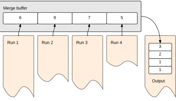
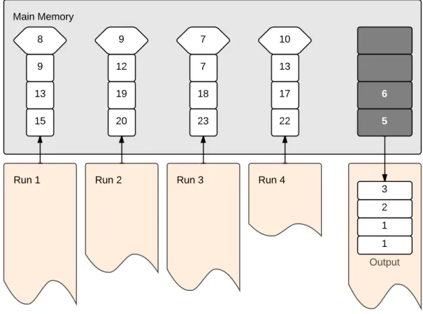
Figure 2.5: Merging four runs into one output file.
2.2.4 Merge
We turn our attention now to the second phase of external sorting, namely the merge phase. The objective of this phase is to create a final sorted file from the existing runs. Figure 2.5 shows a possible execution of the merge phase. In this example, four runs are generated from the initial unsorted input file. These runs are being read, record by record, into a merging buffer in main memory. The smallest record in the buffer is the one with key value5, and is the next one moved to the output file, which in turn is a new run. Then, we move a new record from the top of run 4 into the place where record 5
was located. The execution repeats until only one run is left, which is the sorted output. In order to select the smallest current record, at leastrcomparisons must be performed, since this is the number of runs produced. In [7], Knuth advises making this selection by comparing the records against each other (inr−1 comparisons) only for a small number of runs. When the number of records is larger than a certain threshold (Knuth says 8 in [7]), the smallest record can be determined with fewer comparisons by using aselection tree. In this case, a heap data structure can be employed, in the exact same way as done in run generation with replacement selection. With a selection tree we need only log(r) comparisons, i.e., the height of the tree. Consider now an example of a four-way merging with a two-level selection tree in Figure2.6 (adapted from [7]). We replace the smallest record by its successor record in its run at every step after this, and update the tree accordingly.
Figure 2.6: Four-way merging with a two-level selection tree
Complete the tree by executing the necessary comparisons in the first step. Replace the smallest record by its successor record in its run at every step after this, and update the tree accordingly. This two-level selection tree yields 087 as the smallest record in the first step. Move the record to the output and update the three positions where it appears in the tree. Step 2 outputs 154 as smallest record, and the three positions containing 154 are updated. We repeat this process ofselecting andreplacing while the runs are not empty.
A second improvement over the na¨ıve procedure presented is to take advantage of read and write buffers. Givenrruns and a main memory of sizem, one read buffer of size r+1m can be used for each input run. This way, there is still m−(r+1m )r space left for a write buffer. Figure2.7 shows an example of this idea: the main memory can hold 20 records at time; there are four reading buffers (one for each produced run) of 4 records each and one writing buffer capable of holding also 4 records at time. Select the smallest record in memory from the top of the reading buffers (represented by the hexagons) and move it to the write buffer (represented by the shaded rectangles inside the main memory). When a read buffer is empty read the next top four records from the corresponding run. When the write buffer is full, all records contained in it are written to the output file. The second phase of the external sort executes only θ(n) I/O operations. Despite this good result, the algorithm cannot sort inputs of arbitrary size as it is. If the first phase
Figure 2.7: Merging four runs into one output file using read and write buffers.
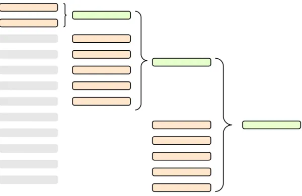
of the algorithm produces more than m−1 runs (ms > m−1), then we cannot merge these runs in a single step. A natural solution for this limitation is to repeat the merging procedure on the merged runs, producing amerge tree. At each iteration we mergem−1 runs into a new sorted run. The result is ms −(m−1) + 1 runs for the next iteration—the total number of runs minus the merged runs in this turn plus the new merged run. At each iteration, we call the total number of possible merges at the same time the merge factor. It is constrained by the size of available main memory: given by ms −1. For a total number of runs r and assuming that r > f actor, the first iteration should attempt to bringrto be divisible by the factor, to minimize the number of merges. The goal is to reduce the number of runs fromr to factor, and then to 1 (the final output). In [21], the number of merges executed in the first iteration is:
f actor0 = ((r−f actor−1)modulo(f actor−1)) + 21 (2.1)
Figure 2.8 show this merging strategy in practice for r = 12 and f actor = 6. In the first iteration we should merge ((12−6−1)modulo(6−1)) + 2 = (5)modulo(5) + 2 = 2
1
The author distinguishes betweenfinal factor andnormal factor. In the query processing context, some operations may consume the output of other operations, and memory must be divided among multiple final merges. We shall not make such distinction in this text.
Figure 2.8: Merging twelve runs into one with merging factor of six.
runs. Other merging strategies, such as cascade and polyphase merges, exist and can be found in [7].
The analysis and implementation presented in Chapters 4 and 5 will focus exclusively on the run generation phase. Since the algorithm used for merging is independent of what is used for run generation, we evaluate sort performance using the same merge algorithm, namely the one implemented by the Hadoop framework.
3.1
Motivation
According to a 2008 study by International Data Corp [22], since 2007 we produce more data than we can store. This huge amount of data was conventionally named big data. Thus the challenge nowadays is not the complexity of the problems to process, but the amount of information to take into account when doing so. In order to solve these data-problems while addressing the inherent problems of distributed computing at the same time, a radical new programming model for processing large data sets with a parallel, distributed algorithm on a cluster—called MapReduce [23]—was conceived. A MapReduce program is defined by two functions: amap and a reduce function. The map function emits records as intermediate key-value pairs, where normally one key is associated to a list of values. The reduce function merges all related intermediate values with the same key to an output value. The MapReduce framework addresses issues as parallel execution, data distribution, and fault-tolerance transparently.
Hadoop is an open source and widely used implementation of MapReduce. It is a soft-ware framework for storing, processing, and analyzing big data. Hadoop partitions large data files across the cluster using HDFS (Hadoop Distributed File System). Data repli-cation increases availability and reliability: if one machine goes down, another machine has a copy of the required data available. The distinction between processing nodes and data nodes tends to disappear as approximately all nodes in the cluster can store and process data. Distributed programs are simpler to write because remote procedure calls are transparently handled by Hadoop. The programmer only writes code for the high-level map and reduce functions. Fault tolerance is achieved by re-assigning failed executions to a different node; nodes which recover can rejoin the cluster automatically.
3.2
Running a MapReduce job
In this section, we overview Hadoop’s architecture and present the entities involved during the execution of a MapReduce job in Hadoop. This overview will provide the basis for a detailed analysis of map and reduce tasks in the following sections.
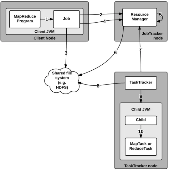
Figure3.1(adapted from [24]) shows the whole process. AClient submits a MapReduce job to the JobTracker, which is responsible for coordinating job execution. The map and reduce functions are spawned astasks to each computing nodes in the cluster, each one running theTaskTrackerservice. The numbered arrows correspond to the following steps:
1. Run job: creates a new instance of theJobClient class;
2. Get new job ID: asks theJobTrackerfor a new ID for the current job;
3. Copy job resources: resources include the job JAR file (a Java package containing the program to be run), a configuration file, and the computed input splits1. An input split is a part of the input that is processed by a single map [24]. They are copied to a directory named after the job ID on theJobTracker’s file system; 4. Submit job: after the JobClient finished all preparation steps, it tells the
JobTrackerthat the job is ready for execution;
5. Initialize job: the JobTracker will enqueue the incoming job, and schedule it according to its current load;
6. Retrieve job splits: this step is necessary so the JobTracker can determine the number of map tasks it should create (one for each split). Reduce tasks are created conform configured;
7. Heartbeat: more than just telling theTaskTrackeris alive, the heartbeat messages tell theJobTrackerwhether theTaskTrackeris ready to execute more tasks. If so,
theJobTrackercommunicates that through a special return value in the message;
8. Retrieve job resources: theTaskTrackerbrings configuration file and the job JAR file and creates a new TaskRunner object;
9. Launch: the new TaskRunner launches a new JVM;
10. Run: the child process keeps theTaskTrackerupdated about the task status until its execution finishes.
Figure 3.1: How Hadoop runs a MapReduce job.
After the job starts to run, theTaskTracker’s child process will keep consuming input splits to feed map tasks. When these tasks are finished, their results are stored locally, on the node’s hard disk and not on HDFS. These results are intermediary key-value records which the reduce phase will bring together.
3.3
Map and Reduce tasks
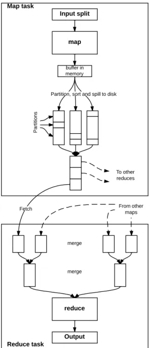
We now zoom inside the MapTask and ReduceTask components in the TaskTracker
node of Figure3.2. Internally, a map task is responsible for more than only running the map function specified by the programmer. In order to make its intermediary results available for the reduce phase, it must organize and prepare these temporary results in a format that can be consumed by reduce tasks.
1
T. White states in [24] that “If the splits cannot be computed, because the input paths don’t exist, for example, then the job is not submitted and an error is thrown to the MapReduce program”.
Figure 3.2: Map and reduce tasks in detail.
The following process happens pipelined, i.e., as soon as one step finishes the next can start using the output emitted by the former. The map function emits records (key-value pairs) while it is processing its input split, and this records are separated into partitions corresponding to the reducers that they will ultimately be sent to. However, the map task does not directly write the intermediary results to the disk. The records stay in a memory buffer until they accumulate up to a certain minimum threshold, measured as the total bytes occupied in the kvbuffer; this threshold is default configured as 80% of thekvbuffer size. When the buffer reaches this threshold, before the map task flushes the records to disk, it sorts them by partition and by key. When the records are sorted, the map task finally writes them to the disk in a file—called spill. Every time the memory
ordered by partition and within each partition by key.
MapReduce ensures that the same reducer receives all output records containing the same key. Figure 3.2 represents this by the dashed arrows going from map to reduce tasks. The attentious reader may ask how do reducers know which TaskTrackers to fetch map output from? The answer is in the heartbeat communication system. As soon as a task finishes, it informs its parentTaskTracker, which will forward the notification to the JobTracker. After the completion of a map task, each reduce tasks will copy its assigned slice into its local memory. However, as long as this copy phase is not finished, the reduce function may not be executed, since it must wait for the complete map output.
Normally, the copied portion does not fit into the reduce task’s local memory, and it must be written to disk. Once all map outputs are copied, the merge phase begins. As we noted in Section 2.2.4, if we have more than m−1 map task outputs, the reduce cannot merge the intermediary results of all maps at the same time. The natural solution is to iteratively merge these spills, as we illustrated in Figure 2.8. We shall give more details about the Hadoop merging strategies in the following sections. Once we have a single merged file, the reduce function is finally called for each key-value of this file and outputted to the shared file system, HDFS.
This whole infrastructure is necessary to accomplish the design goals of MapReduce: distribution, parallelism, scalability and fault tolerance. The user code (map and reduce functions) is a small part in the whole process. Since this work is focused on run generation for external sorting, we shall concentrate on the map task, which is where sorted runs are initially produced.
3.3.1 The Map Side
While a map task is running, its map function is emitting key-value records to an in-memory buffer class calledMapOutputBuffer2. If not explicit specified, all the entities discussed during this section are located inside this class. In the previous section we stated that these records are separated into partitions corresponding to the reducers
2This is true when the MapReduce job has at least one reducer. When there is no reduce phase,
a DirectMapOutputCollector is used which directly writes the records to the disk as the job’s final output.
that they will ultimately be sent to. This is done by a partitioner component, which assigns records output by the map tasks to reducers based on a partitioning function. This function can be customized by a user-defined partitioning function, but T. White states in [24] that “normally the default partitioner—which buckets keys using a hash function—works very well”.
After the record receives a partition, the collector adds the record to an in-memory buffer: an unordered key-value buffer (kvbuffer). Hadoop keeps track of the records in the key-value buffer in two metadata buffers for accounting (kvindices and kvoffsets).
Kvbuffer is a byte array that works as the main output buffer: the keys and values of the records are serialized into this buffer. The amount of memory reserved for the kvbuffer
is calculated by:
io.sort.mb−(io.sort.mb×io.sort.record.percent
16 ) (3.1)
Hadoop’s default value for the io.sort.mb property is 100MB and for the
io.sort.record.percent is 0.05%. This configuration yields a kvbuffer of 104,529,920 bytes. The accounting buffers (or metadata buffers) are auxiliary data structures used by Hadoop to efficiently manipulate the key-value records without actually having to move then in the kvbuffer. They are composed of two integer arrays. The first array,
kvindices, has three integer values (4 bytes each): partition,key start (a pointer to where the key starts in the kvbuffer), andval start (a pointer to where the value starts in the
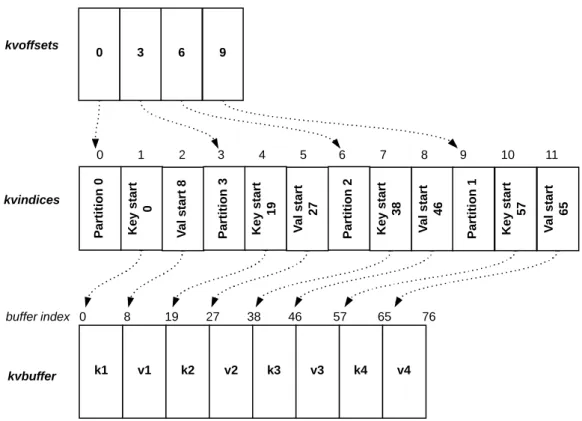
kvbuffer). The second array, kvoffsets, manages a further level of indirection pointing to where each hpartition, keystart, valstarti tuple starts in the kvindices (also 4 bytes integer pointer). An illustration of how these buffers are used is given in Figure 3.3, which shows 4 key-value pairs already serialized in the kvbuffer, where each key is 8 bytes long and each value is 11 bytes long. The kvindices buffer keeps track of where each record’s key and value starts and also to which partition that record belongs to. Finally in the kvoffsets buffer there is second round of pointers indicating where each of thehpartition, keystart, valstarti tuples are located in the kvindices. The number of records in the metadata buffers is calculated by:
io.sort.mb×io.sort.record.percent
16 (3.2)
The default configuration values result in a capacity to store metadata of 327,680 records, i.e., 5% of the reserved space. We call attention for the obvious although impor-tant difference between the buffers: the kvbuffer is measured in bytes, while accouting buffers are measured in records. As we shall see in the following paragraphs, the spill procedure is triggered when one of these buffers—thekvbuffer or thekvindices—reaches
Figure 3.3: In-memory buffers: key-value (kvbuffer) and metadata (kvindices and kvoffsets).
a configurable threshold. The default configuration expects a record with average size around 320 bytes. However, if the average size is much smaller than the originally ex-pected, thekvbufferwill never get full enough to trigger the spill procedure. But because the metadata buffer threshold is measured in number of records, and now more records fit in the kvbuffer at the same time (because they are smaller), kvindices will trigger the spill all the time. This is a waste of resources: we have an approximately empty byte buffer and a full accounting buffer to track the records in it. In order to avoid this misuse of the available space, given by the io.sort.mb property, we can simply increase
io.sort.record.percent. To optimize this value, Hadoop provides useful statistics gener-ated during job execution by means of counters. Two counters are useful here: map output bytes, the total bytes of uncompressed output produced by all maps in the job; and map output records, the number of map output records produced by all the maps in the job. Thus we can calculate the average size of a record by M apOutputRecordsM apOutputBytes . The collector serializes the key-value records in thekvbuffer. It also adds metadata (the position where the key and value start in the serialized buffer) about kvbuffer to kvin-dices and adds metadata (where each metadata tuple hpartition, keystart, valstarti) about kvindices tokvoffsets. When the threshold of accounting buffers or record buffer
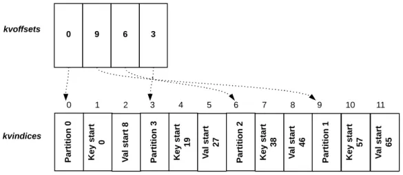
Figure 3.4: Kvoffsets buffer sorted by partition.
is reached, the buffers are spilled to disk. The io.sort.spill.percent configuration prop-erty determines the threshold usage proportion for both the key-value buffer and the accounting buffers to start the process of spilling to disk [24]. The default value of this property is 80%, which is used as asoft limit. The collector will continue to serialize and keep track of new records emitted by the map function while a spill thread is working until the buffers are full, when the hard limit is reached. The collector then suspends its activity then until the spill thread has finished.
The purpose of the second accounting buffer is to improve CPU performance. We mention in section 3.3 that records should be ordered by partition and, within each partition, by key. For the run generation inside map tasks, Hadoop uses quicksort. C. Nyberg et al. explore optimization techniques with respect to sorting in [13]. Two of these techniques include the minimization of cache misses and the sorting of only pointers to records rather than the whole records. They adopted quicksort in [13] because “it is faster because it is simpler, makes fewer exchanges on average, and has superior address locality to exploit processor caching”. These techniques are also employed by Hadoop— the second accounting buffer holds the pointer values exchanged by the sort algorithm. This so-calledpointer sort technique is better than a traditional record sort because it moves less data. When sorting kvoffsets, quicksort’s compare function determines the ordering of the records accessing directly the partition value inkvindices through index arithmetic. But quicksort’s swap function only moves data in the kvoffsets.
We return to Figure 3.3 as an example. The records in the kvindices buffer are not ordered by partition: these are 0, 3, 2 and finally 1. Initially, kvoffsets is sorted with respect to the order which the records where inserted into kvindices. Sorting it results in the state shown in Figure 3.4.
key-value records, one last spill is executed to flush the buffers. The map task then has several spill files in its local disk, which must be merged into a final output file that becomes available for the reducers. Hadoop implements an iterative merging procedure, where the propertyio.sort.factor specifies how many of those spill files can merged into one file at a time.
The map side merge work as follows: first an array with all spill files is obtained. In the case where there is only one spill file, that spill is the final output; otherwise, two final output files are created: one for the serialized key-value records (final.out), and another for pointing where each partition starts in the former (final.out.index). As a header, numberOf P artitions×headerLenght bytes are reserved in the beginning of both files. The numberOf P artitionsis equal to the number of reducers configured for the job; theheaderLenghtis a constant value set in 150 bytes. First, an output stream is created to write the final file. Then, for each partition, a list of segments to be merged is created and, for each spill, a new segment is added to the segment list. Each segment correspond to a “zone” in each spill file corresponding to the current partition. Figure 3.5 illustrates the idea. We now call the merge method in theMerge.class, passing the segment list. Note: we are still inside the loop over partitions. This means that as many mergings as the number of partitions will be executed.
The merge procedure calculates the number of segments to merge in the first pass using equation 2.1. We reintroduce the term f actor (abbreviated to f), now in the context of Hadoop. Its value is configured through the io.sort.f property, and it corresponds to the maximum number of streams to merge at once. Assuming we have more than f segments, the first merge pass brings the total number of runs to an amount divisible by f−1 (each pass transformsf runs into one) to minimize the number of merges which, in turn, minimizes disk access. We refer to the number of runs to be merged in the first pas as thefirst factor. All the subsequently passes will then merge f streams.
First-factor segments are copied from the original segment list to an auxiliary list (called
segments-to-consider). Then, all segments in this list are added to a priority queue. The heap which implements the priority queue sort the segments ascending by size, thus smaller segments sort first. All records from the priority queue are written into a temporary file, and the heap is cleaned afterwards. This temporary file is a new, merged segment, which is added to the list of segments to be merged. After some clean-up routines are executed, the second round of merge starts.
Figure 3.5: Two spill files and the resulting segments for each partition.
At some point, there will be fewer segments than f, wich means the merge reached the last merge level. When this occurs, the segments are already in the heap and, instead of creating another temporary file, we simply return the priority queue back to the
MapTask.class. Each segment is pulled from the priority queue and is written to the final file. Here, the loop around the partitions finally ends. Some housekeeping functions are executed, and the next iteration —with the next partition— can begin.
We show one example of a merge tree in Figure 3.6. Assume for a given partition (say 0) we built a segment list of size 20 (we have at least 20 spill files with records that belong to partition 0) and anio.sort.factor of 10. Equation2.1 yields ((20−10−
1)modulo(10−1)) + 2∴(9modulo9) + 2∴2, which means we must merge two segments in the first round. Given the (sorted ascending by file length) segments list, we get the first two and merge them. Then, we merge the next 10 segments. At this point, we have 8 segments from the original list and 2 temporary ones, resulting from the previously merged segments. As expected, this sums exactly to 10 segments, which are now merged in the final file.
Figure 3.6: Merge tree with 20 segments and merge factor 10.
This concludes the map task, after which theTaskTrackersends a heartbeat informing theJobTracker. Next time a reducer consults theJobTracker, it will be informed that in a givenTaskTrackerthere are map outputs ready to be copied. We close this chapter presenting figure 3.7, which summarizes the map-side processing we have discussed so far.
3.4
Pluggable Sort
TheMapOutputBufferclass is Hadoop’s default implementation of in-memory sort and
run generation, which was fixed since its first version. However, the second stable ver-sion of Hadoop (2.x) enables the customization of this procedure through an interface called pluggable sort. It allows replacing the built-in run generation logic with alterna-tive implementations. This means not only having the possibility to customize which data structures and buffer implementations to use, but also which sort algorithm. The pluggable sort was proposed by SyncSort [25] and discussed and develop in Apache’s JIRA issue tracker under codename MAPREDUCE-2454 [26].
A custom sort implementation requires a MapOutputCollector implementation class, configured through the property mapreduce.job.map.output.collector.class. Since all pluggable components run inside job tasks, they can be configured on a per-job ba-sis [27]. Likewise, custom external merge plugins can also be customized for reduce tasks.
key-value pairs to emit. When the map task calls this method, it is giving the output buffer a chance to spill any record left in the buffer, and telling the buffer to merge all spill files (or, in the case there is only one spill, rename it). Theclose method simply performs some housekeeping procedures, closing streams and freeing class fields. Using this extensibility mechanism, we implement run generation using the replacement-selection algorithm, as an alternative to the original quicksort. Because of Hadoop’s own big data nature, having multiple spill files is the rule and not an exception. Thus, not only an alternative output buffer has to take care of sorting in-memory keys and partitions but also merging these multiples sorted spills into one single, locally-ordered file. It has to carefully consider data structures to store the records and algorithms to manage and reorder these records. It should be clear that this merge is only a local merge (performed by each map task). A second, cluster-wide merge performed in the reduce side will merge the locally-ordered files that each map task has processed. This global merge, however, is beyond the scope of this work, where we focus exclusively in the map side task sorting and merging. In the next chapter, we introduce our own replacement-selection-based implementation of MapOutputBuffer
Implementation
This Chapter describes four implementation approaches for run generation in Hadoop using replacement selection. Starting with a na¨ıve approach, where memory manage-ment is left under complete control of the Java virtual machine, each implemanage-mentation introduces an addition in complexity in order to improve performance
During the discussion, we compare the current algorithm with Hadoop’s original output buffer. Our objective in this Chapter is to construct an output buffer which can generate a small number of larger runs if comparable to Hadoop as fast as possible. The lesser number of spills created by replacement selection leads to a faster merger phase [28]. This suggests that if we decrease the difference in the run generation phase, possibly the total execution time of our custom buffer will be shorter than Hadoop’s buffer execution time. The best trade-off between generating faster runs or generating less spill files is one of the questions this work tries to solve.
4.1
Development and experiment environment
The tests in this Chapter were executed in a machine with the following configuration:
• Architecture: Intel(R) Xeon(R) 64bits CPU X3350 @ 2.66GHz with 4GB of main memory and 465GiB hard disk;
• Operating System: Ubuntu 12.04 LTS Linux (3.0.0-12-generic-pae) i386 GNU/Linux
• Java Version: 1.7.0 25 OpenJDK
Figure 4.1: The setup of the tests performed in this Chapter. We feed the output buffer with records directly from the input reader.
In order to isolate the performance analysis to the run generation phase, we perform micro-benchmarks instead of complete Hadoop jobs. We show an example of the set up in Figure 4.1, only replacing the random strings for some pleasant text. Records are read directly from an input file and fed into Hadoop’s collect method, simulating the output of the Map phase. The collect method triggers run generation and the merge of local output files, after which the Reduce phase starts. In our experiments, the process stops when runs are generated and timestamps are collected to measure run generation execution time.
The input is a 9GB file with randomly generated strings varying length between 80 and 160 bytes (one string per line). The in-memory buffer is 16MB, which yields a ratio of 562.5 between input and buffer size. The keys in our experimental job are the full strings, and the values are 1.
4.2
Record Heap
The Record Heap implementation is characterized by a simplistic and direct implemen-tation of replacement selection, fully relying on the Java Virtual Machine (JVM) to perform memory management and on container classes of the Java Standard library.
The RecordHeap class implents the MapOutputCollector interface, and is the class
plugged into the Hadoop’s job. Besides it, there are other two important classes: the
HeapEntry class and the NaiveReplacementSelection class. The first class
encapsu-lates the record’s key, value, partition and current status (a Boolean flag). The former class implements the replacement selection algorithm and has the following main fields:
• A priority queue of HeapEntry objects: each hkey, value, partitioni tuple is en-capsulated in aHeapEntry object and put intoPriorityQueueinstance, which is Java’s default priority queue. In this implementation, both the record buffer and
the selection tree entities are implemented into one single object — this queue. As the priority queue is supported by a heap, we shall use both terms indistinctly;
• AHeapEntry comparator: records are sorted by status (active < inactive), parti-tion, and key within the heap.
• AHeapEntryextra object: where we save the last output record, used to compare
and decide if the incoming record belongs to the current run or not;
• A Boolean flag for the current active status: we detected that all the records are inactive when the status of the top element pulled from the PriorityQueue is different from the current status flag. If so, we simply set the current active status to the top element’s status. This saves the work of iterating through the heap to flip all statuses.
• A writer: this is a synchronous writer to output the records as spill files. We open a stream when we create a new run and keep appending key and values into it. Hadoop creates index objects of where each partition begins and ends (begin plus length) in the spills (as shown in Figure 3.5). We made sure to mimic Hadoop’s file format to be able to use the same merger later.
The process works as follows: as the map function emits new key/value pairs, the map task pushes them into the output buffer through the collect method. The collect method calls anadd method in theNaiveReplacementSelectionobject which encapsulates the key, the value, and the partition in a new HeapEntry object and puts it into the heap. Java’s defaultPriorityQueueimplementation does not limit the number of elements it can contain1, thus we control the maximum number of HeapEnty objects in the heap with a variable max buffer size. The priority queue will have a constant number of elements from the moment the buffer is full (i.e., the number of elements in the heap is equal to the buffer maximum size) for the first time until the moment when the map tasks call the flush method.
Once the heap is full, we have to make space for the incoming records. Pulling the priority queue yields the lowest possible record, which is written out. Then, the incoming record is compared to the saved record: if the new record is bigger than the saved record, it still belongs to the current run. Then, its status is set to active and the record is added to the heap. Otherwise, add it with inactive status. At any time, if the pulled record’s status is not equal to the current active status, close the run, flip the current active status and start a new run.
1The PriorityQueue grows as needed, doubling it size when it is has less than 64 elements and
0 100 200 300 400 Hadoop RecordHeap
Execution time (in seconds)
Buffer algorithm
Figure 4.2: Comparison between Hadoop’s MapOutputBuffer and our customRecordHeap
buffer.
method. The process to flush the priority queue is similar to the previous one. The just pulled record is compared to the saved record to decide if it belongs to the current run or not. If so, the record is outputted and the saved record is updated. If not, the run is closed and a new one is started. This executes while the priority queue is not empty. Figure4.2shows a comparison between Hadoop’s default output buffer and the RecordHeap implementation, as we can see Hadoop’s run generation is 60% faster, which is approximately 300 seconds. We shall now investigate what is the cause of this difference.
Both the key and the value in Hadoop are generic objects which may assume any of the job’s configurable types, like Text, LongWritable2, and IntWritable. Hadoop reuses this pair of objects when feeding the map function with data from the input split. The
RecordReaderclass provides a record iterator with some extra capabilities, like parsing a CSV input for example. The map task uses a RecordReader to generate record key-value pairs, which it passes to the map function. TheRecordReader instantiates a key object and a value object when the mapper function first asks for records. Writable types, in general, are backed up by a byte array and provide aset method, which copies the received set method’s argument into the byte array. When these objects arrive to the collect method in the MapOutputBuffer class, they are serialized into the kvbuffer
(i.e., their bytes are copied to the MapOutputBuffer’s byte array). When the mapper asks for more records from the RecordReader, the existing key and value objects are reused — the data read from the input is set into these objects. This saves Hadoop from creating new objects for each record read, which is not true for the RecordHeap
implementation.
Recall that the buffer and the selection tree of theRecordHeapare one single object, an instance of Java’sPriorityQueueclass strongly typed withHeapEntryobjects. Adding these recycled key and value objects to the buffer provokes an erroneous behavior: since
2
Writableis the interface created to handle data serialization in Hadoop. It has two methods: one for writing to a DataOutput binary stream and one for reading from a DataInput binary stream [24]. We shall discuss serialization in more detail in a further Section.
(a)Memory monitor during execution of MapOutputBuffer.
(b)Memory monitor during execution of RecordHeap.
Figure 4.3: Java’s heap space in two different scenarios. In foreground at the lower part of the figure there is the used heap, and the background there is the heap size.
the key and the value are instantiated in theRecordReaderonly once, their objects hold the same reference during the whole execution (until they are destroyed). Thus, every “new” record key-value pair added to our buffer points to the same object. This results in allHeapEntry instances in thePriorityQueuehaving the same key and value as the last added one. The natural solution to this problem is to create new objects every time theRecordReaderreads data from the input. It turns out that the price to pay in terms of performance for creating so many objects is expensive.
In these tests we decrease the input file to 2GB and used the VisualVM 1.3.7 profiler tool [29] with the Visual Garbage Collection Monitoring Tool plugin [30] to monitor the execution. Figure4.3compares the JVM heap space during the execution of a test with Hadoop’s MapOutputBufferclass and our RecordHeapoutput buffer.
The right side of the figure (4.3b) shows theRecordHeapexecuting over the same input, but having an entirely different memory footprint. The used Java’s heap space constantly reaches 600MB, in contrast with left side of the figure (4.3a) where the used heap is stable at 50MB. It is not the high memory consumption which overloads the system and brings performance down, but instead the high volume of memory allocations and deallocations in JVM’s heap of short-time objects. One can wonder that each memory peak correspond to one run and, when a spill finishes, a lot of memory is freed at once. However, we recall that the number of records in the buffer stays approximately constant during all the collection phase. For every incoming record only one existing record is selected and replaced in the buffer. What happens in fact is that every time we replace a record (appending it to the current open run) it is polled from the priority queue; since we are constantly inserting new records in the buffer, we are also constantly removing
promising: we have already saved some time in the merging phase. In the next Section, we try to solve the excess of garbage collection by splitting the buffer from the selection tree. The first will be responsible only for storing records, while the former will provide access to the records as well information about the current run, the current partition and other necessary fields to execute the algorithm.
4.3
Pointer Heap
Hadoop reuses the same key-value pair4 to send the data from the input to the buffer. It does not have to create a new pair for each record it emits because the key and the value are serialized into the buffer. This means the records are read, turned into a byte array, and copied to the buffer. To follow this strategy and avoid creating a massive number of objects, we split the solution from the previous Section: a new byte array will mimicMapOutputBuffer’s kvbuffer behavior, being a placeholder for the serialized keys and values, while in a priority queue we insert only metadata about the current record and current spill. This metadata includes the current run number, the record partition, andpointers to where the values are located in the buffer — which lead us to name this solution PointerHeapbuffer.
Replacement selection is based on the premise that when we select the smallest record from the buffer, we can replace it with the incoming record. However, this is only valid if all the records have the same size, i.e., they are fixed-length. This is not true for our experiments and often not true in real world jobs, specially when dealing with text. Manage efficiently the space in the buffer when records are of variable length becomes a necessity. To address this issue, we implemented a memory manager entity based on the design proposed by P. Larson in [9]. This memory management is not an issue in
MapOutputBuffer’s quicksort strategy because the records are appended in the end of
the buffer as they come and, when they are removed, they are all remove at once (when a spill is triggered). Thus, Hadoop is free from this extra overhead we shall detail now.
3The Java’s garbage collector is multi-strategy, complex entity based on the concept ofgenerations.
GC runs first in young generations, and objects that survive (i.e., another object still holds a reference to them) are promoted to older generations. A common strategy to trigger garbage collection is to run the collector when memory allocation memory fails. Further references can be found in [31–33].
4
In a real world job, where the map function is actually executed, there is one key-value pair transmit-ting data between theRecordReaderand the map function and another pair between the map function and the in-memory buffer.