Volume 2 - Issue 6, June 2015
16
Hybridizing Tabu Search with Ant Colony Optimization for
Solving Job Shop Scheduling Problems
Prof.C.Sivaprakasam
1Dr.V.P.Eswaramoorthy
2Abstract: -
The prime contributor to the development of the competitive market is the manufacturing industry which requires a good schedule. Scheduling is the allocation of resources to activities over time. Scheduling is considered to be a major task done to improve the shop-floor productivity. The job shop problem is under this category and is combinatorial in nature. Research on optimization of the job shop problem is one of the most significant and promising areas of optimization. This paper presents an application of the global optimization technique called tabu search that is combined with ant colony optimization technique to solve the job shop scheduling problems. The neighborhoods are selected based on the strategies in the ant colony optimization with dynamic tabu length strategies in the tabu search. The inspiring source of ant colony optimization is pheromone trail that has more influence in selecting the appropriate neighbors to improve the solution. The performance of the algorithm is tested using well known benchmark problems and also compared with other algorithms in the literature.
Keywords: Tabu List; Neighborhood Structures; Tabu Length; Pheromone Trail; Makespan.
1. Introduction
Tabu Search (TS) is a meta-heuristic approach used to solve combinatorial optimization problems and was first described in 1986 [1]. TS provides solutions very close to optimality and is used to tackle the difficult problems. These successes have made TS extremely popular among those interested in finding good solutions to the large combinatorial problems encountered in many practical settings. TS is based on Local Search (LS) improvement techniques. LS can be roughly summarized as an iterative search procedure that, starting from an initial feasible solution, progressively improves it by applying a series of local modifications (or moves). At each iteration, the search moves to an improving feasible solution that differs only slightly from the current one. In LS, the quality of the solution obtained and computing times are usually highly dependent upon the “richness” of the set of transformations (moves) considered at each iteration of the heuristic.
The Ant Colony Optimization (ACO) algorithm is a distributed algorithm used to solve NP-hard combinatorial optimization problems. The ACO uses a population of co-operating ants also known as agents. The cooperation phenomenon among the ants is called foraging and recruiting behavior [2, 3]. This describes how the ants explore the world in search of food sources, then find their way back to the nest and indicate the food source to the other ants of the colony. To do so, the ants use an indirect way to communicate through tracks of pheromone, a chemical substance that they can deposit on their paths. Each ant deposits a fraction of pheromone on the way back to the nest so as to indicate the source to the others. Hence the pheromone information plays major role in finding the shortest path from the food to the nest.
The job shop problem consists in scheduling a set of jobs on a set of machines with the objective to minimize the makespan which is the maximum completion time needed for processing all jobs, subject to the constraints that each job has a specified processing order through the machines and that each machine can process at most one job at a time. In this paper, a new heuristic algorithm, which hybrids the tabu
search method and the ant colony optimization (HTSACO), is proposed. The ACO method is used to select neighborhood solution in TS. This paper is structured as follows. In section 2, the JSSP is explained and is formally described. In section 3 literature review is given. In section 4, TS method and ACO are described. In section 5, implementation of the HTSACO to the JSSP is given with the algorithm using the proposed method. In section 6, experimental results and discussion of the proposed method is given and finally the conclusion is given in section 7.
2. Problem Definition and Notation
The standard model of the job shop problem is demoted by n/m/G/Cmax, where n is the total number of jobs,
m is the total number of machines, G is the technological matrix denoting the processing order of machines for different jobs. The matrix G can be represented as follows.
M2 M3 M1
G = M1 M2 M3
M3 M1 M2
Each row of G represents a job. Cmax is the makespan representing completion time of the last operation in the job shop. Each job consists of a sequence of operations, each of which has to be performed on a given machine for a given time. A schedule is an allocation of the operations to time intervals on the machines.
The processing of an operation i on a machine j is denoted by uij and we can form a relation uipuiq
representing uiq is directly immediate to uip. Let ij be the
processing time of the operation uij. The value Cij = Cik+ij
denotes the completion time of uij in the relation uikuij. The completion time of all Cij will be found. Then Cmax is calculated as in the equation (1)
Volume 2 - Issue 6, June 2015
17 all uijV
The main aim is to minimize Cmax value. Let J be the set of jobs (1,2,…,n}, M be the set machines (1,2,…,m}and V be the set of nodes {0,1,2,…,ñ+1} where o and ñ+1 are the dummy nodes representing start and finish operations respectively. It is useful to represent the job shop scheduling problem in terms of a disjunctive graph D = (V, A, E).A is a set conjunctive arcs representing the precedence of operations in the job and E is a set of disjunctive edges with no direction representing possible precedence constraints among the operations belonging to different machines.Let us consider an example of the JSSP with 4 jobs and 3 machines. The data are given in table 1.
Table 1
Table 1. Processing times and operation sequence for a 4x3 instance
Job Processing Sequence
J1 (1,2) (2,3) (3,4)
J2 (3,4) (2,4) (1,1)
J3 (2,2) (3,2) (1,3)
J4 (1,3) (3,3) (2,1)
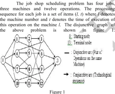
The job shop scheduling problem has four jobs, three machines and twelve operations. The processing sequence for each job is a set of items (l, t) where l denotes the machine number and t denotes the time of execution of this operation on the machine l. The disjunctive graph of the above problem is shown in figure 1.
Figure 1
In the graph vertices drawn as circles represent tasks. Conjunctive arcs, which are directed lines, represent precedence constraints among the tasks of the same job. Disjunctive arcs, which are undirected lines, represent possible precedence constraints among the tasks belonging to different jobs being performed on the same machine. Two additional vertices are drawn to represent the start and the end of a schedule.
3. Literature Review
Number of researchers have adopted this TS technique for solving the job shop scheduling problem. Glover [1, 4, 5] presented the fundamental principles of Tabu Search as a strategy for combinatorial optimization problems. In his work, the major ideas and findings to date, and the
challenges for future research were presented. Part I of his work dealt with basic principles, ranging from the short-term memory process at the core of the search to the intermediate and the long term memory processes for intensifying and diversifying the search and the illustrative ideas for implementing the tabu conditions that underlie the processes. Part II dealt with more advanced considerations, applying the basic ideas to special settings and outlining the dynamic move structure to insure finiteness. Ferdinando Pezzella and Emanuela Merelli [6] proposed a new procedure based on the tabu search method and the shifting bottleneck procedure (TSSB). The integration of the shifting bottleneck procedure in tabu search framework aims to use qualitative information extensively during the local search. In this method, the tabu search technique uses the shifting bottleneck procedure to determine the initial solution and subsequently to reoptimize locally the sequence of each machine belonging to the critical path. The TSSB algorithm is composed of three fundamental modules. The first implements the shifting bottleneck procedure and then generates the initial solution, the second implements the local search based on the TS technique and third reoptimizes locally the sequence of each machine whenever a better solution is provided by second module.
Calderia et al [7] presented Tabu-Hybrid using one of the representation for the JSSP called permutation with repetition (PWR) in which the order of operations within the permutation is interpreted as a sequence for building a schedule solution. The decoding procedure scans each permutation from left to right and uses sequence information to build a schedule consecutively. The simple permutation of operations normally leads to infeasible schedules because an operation can only be scheduled if its predecessors have already been scheduled. This problem is avoided by using permutation with repetition in which the operations are represented by the identifier of the job they belong to. This representation covers all feasible sequences for any JSSP instance. There is however a large redundancy in this representation. The total amount of different permutations is much larger than the number of possible sequences. Eugeniusz Nowicki et al [8] presented i-TSAB algorithm which is an extension of their earlier landmark TSAM algorithm. In addition to the short-term memory mechanism found in all implementations of the tabu search, i-STAB is characterized by the following algorithmic components: (1) the highly restrictive move operator, (2) re-intensification of search around previously encountered high-quality solutions and (3) diversification of search via path relinking between high-quality solutions. i-TSAB is largely deterministic. The only possible sources of randomness involve tie-breaking at specific points during the search.
Volume 2 - Issue 6, June 2015
18 algorithms. VinmH cius Amaral Armentano et al. [11] presented a tabu search approach to minimize total tardiness for the job shop scheduling problem. The method uses dispatching rules to obtain an initial solution and searches for new solutions in a neighborhood based on the critical paths of the jobs. Diversification and intensification strategies are suggested.
Christian Blum et al. [12] proposed MAX-MIN ant system in the hyper-cube framework approach to tackle the broad class of group shop scheduling problem instances. It probabilistically constructs solutions using the non delay guidance which employs the black-box local search procedures for improving the constructed solutions. Ventresca and Ombuki [13] presented an ant colony optimization algorithm approach to the job shop-scheduling problem. The main goal was to examine pheromone-updating techniques and their effects on solution space exploration. A rudimentary Ant System was examined along with a Max-Min Ant System approach. A new technique called Foot Stepping was proposed that improves the solution quality of the ant system. Jun Zhang et al [14] presented an investigation into the use of an ACS to optimize the JSSP. The main characteristics of this system are positive feedback, distributed computation, robustness and the use of a constructive greedy heuristic. The results have shown that the performance of the ACS for the JSSP largely depends on the parameter values and the number of the ants. Adjusting these parameter values takes a great deal of time, the optimal parameter values depend on the problem to solve, and it is difficult to find an all-purpose setting of parameters for all problems.
4. The Strategies
4.1 Tabu Search
Tabu search (TS) is a metaheuristic approach and global iterative optimization method designed to find an optimal solution for combinatorial problems. This method has been suggested and refined by Glover [1, 4, 5]. The basic principle of TS is to pursue Local Search, whenever it encounters a local optimum by allowing non-improving moves. The important elements of TS are described below.
4.1.1 Neighbors and neighborhood structure
The search space is simply the space of all possible solutions that can be considered during the search. In the search space a neighbor si (0 < i < k) is defined by a pair (x, y) provided x and y are successive operations on a machine and on some critical path in the graph G. The critical path is a longest path from the node 0 to the node ñ+1 corresponding to the makespan of the constructed solution. Let L(S) be the set of neighbors that can be applied to the current solution. The neighborhood is defined by the processing orders of operations at the time of application of a neighbor si to the current solution. At each iteration, the application of each neighbor siL(S) define a set of neighboring solutions in the search space.
4.1.2 Tabus
Tabus are one of the important elements of TS and are used to prevent cycling. One can avoid cycling by declaring the tabu moves that prevent the application of recent neighbors which are called forbidden neighbors. Tabus are stored in a short-term memory of the search space (the tabu list) and usually a fixed and fairly limited quantity of information is recorded. In any given context, there are several possibilities regarding the specific information that is recorded. One could record complete solutions, but this requires a lot of storage and makes it expensive to check whether a potential move is tabu or not; it is therefore seldom used. The most commonly used tabus involve recording the last few neighbors which are not applied for transformations performed on the current solution and prohibiting the reverse transformations.
4.1.3 Variable tabu list size
The basic role of the tabu list is to prevent cycling. The fixed length tabus can not prevent cycling [4, 5]. We can observe that if the length of the list is too small, cycling can not be prevented and long size tabu creates many restrictions so as to increase the mean value of the visited solutions. An effective way of removing this difficulty is to use a tabu list with variable size according to the current iteration number. The length of the tabu list is initially assigned according to the size of the problem and it will be decreased and increased during the construction of the solution so as to achieve better exploration of the search space.
4.1.4 Aspiration criteria
While central to TS, the tabus are sometimes too powerful that they may prohibit attractive moves, even when there is no danger of cycling, or they may lead to an overall stagnation of the searching process. It is thus necessary to use algorithmic devices that will allow one to cancel the tabus. These are called aspiration criteria. The simplest and most commonly used aspiration criterion consists in allowing a move, even if it is in tabu, if it results in a solution with an objective value better than that of the current best-known solution. Much more complicated aspiration criteria have been implemented by different research persons and successfully implemented [15], but they are rarely used.
4.1.5 Termination criteria
In theory, the search could go on forever, unless the optimal value of the problem at hand is known beforehand. In practice, obviously, the search has to be stopped at some point. The most commonly used stopping criteria in TS are given as follows:
(i) a fixed number of iterations (or a fixed amount
of CPU time);
(ii) after some number of iterations without an
Volume 2 - Issue 6, June 2015
19 (iii) when the objective reaches a pre-specified
threshold value.
4.2 Ant Colony Optimization
4.2.1 Fundamentals of Ant Colony Optimization
For solving the combinatorial optimization problems, the Ant Colony Optimization (ACO) is used for designing metaheuristic algorithms. The first algorithm was presented in 1991 [16, 17] and since then, different methods of the basic principle have been reported in the research field. In analogy to the biological example, ACO is based on the indirect communication of a colony of simple agents, called (artificial) ants, mediated by (artificial) pheromone trails. The inspiring source of ACO is the “pheromone trail laying and following” behaviour of the real ants, which use the pheromone as a communication medium. Some amount of the pheromone will be deposited by the ants on their paths. The probability for choosing the next path by an ant will be directly proportional to the amount of pheromone on that path.
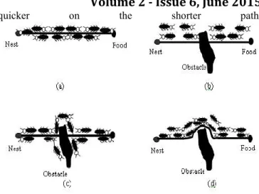
Also the ants are capable of adapting to changes in the environment, for example finding a new shortest path once the old one is no longer feasible due to a new obstacle on the way. Figure 2 explains the behaviour of the real ants. The ants are moving on a straight line which connects a food source to the nest (Figure 2a). As stated each ant probabilistically prefers to follow a direction rich in pheromone rather than a poorer one. This elementary behaviour of real ants can be used to explain how they can find the shortest path which reconnects a broken line after the sudden appearance of an unexpected obstacle interrupting the initial path (Figure 2b). Once the obstacle has appeared, those ants which are just in front of the obstacle cannot continue to follow the pheromone trail and therefore they have to choose between turning right or left (Figure 2c). In this situation half the ants may be expected to turn right and the other half to turn left. The very same situation can be found on the other side of the obstacle. It is interesting to note that those ants which choose, by chance, the shorter path around the obstacle will more rapidly reconstitute the interrupted pheromone trail compared to those which choose the longer path. Hence, the shorter path will receive a higher amount of the pheromone in the time unit and this will in turn cause a higher number of ants to choose the shorter path (Figure 2d). Due to this positive feedback, very soon all the ants will choose the shorter path. Although all ants move at approximately the same speed and deposit a pheromone trail at approximately the same rate, it is a fact that it takes longer to contour obstacles on their longer side than on their shorter side which makes the pheromone trail accumulate quicker on the shorter side. It is the ants’ preference for higher pheromone trail levels which makes this accumulation still
quicker on the shorter path.
Figure 2. Adapting to the changes (a) Ants travel in a shortest path. (b)An obstacle appears on the path and ants
choose left or right path with equal probability. (c) Pheromone deposited in the shorter path is more than longer
one. (d) All ant choose the shorter path.
4.2.2 State transition rule
The ant algorithm can be represented into a graph, in which the ants move along every branch from one node to another node and so construct paths representing the solutions. Starting in an initial node, every ant chooses the next node in its path according to the state transition rule by using probability of transition. Let S be the set of nodes at a decision point i. The transition probability for choosing the edge from the node i to the node j by an ant is calculated as given in equation (2)
((i, j) α (( j)) β
if jS
∑ ((i,j)) α ((j)) β P(i, j) = jS
(2)
0 otherwise
(i, j) is the quantity of the pheromone on the edge between the node i and the node j. (j) is the inverse of the operation time of the node j. and tune the relative importance in probability of the amount of the pheromone versus the operation time. According to this rule, the artificial ants move to the node that has a higher amount of pheromone and lesser value of the operation time and will have a higher probability to be scheduled in the partial solution.
4.2.3 Global updating rule
Volume 2 - Issue 6, June 2015
20 by applying the global updating rule given in the equation (3) which is used in our proposed method.
τ(i, j)t = τ(i, j)t-1 + (1-ρ).q/Lk (3)
ρ is the coefficient representing pheromone evaporation (note: 0 < < 1). q is a value chosen randomly with uniform probability in [0,1]. Lk is the minimum tour length. Hence the amount of the pheromone deposited on each edge is inversely proportional to the length of the path so as to enable the shorter path to get higher amount of the pheromone deposited on the edges.
4.2.4 Local updating rule
The evaporation phase is substituted by a local updating rule of the pheromone applied during the construction of the solution. In each time t, the ant moves from the node i to the next node j in the graph D, the pheromone associated to the edge is modified according to the equation (4).
τ(i, j)t =(1-).τ(i, j)t-1 + ρ.τ0 (4)
τ0 is the initial pheromone value and is defined as τ0=n/L,
where L is the tour length produced by the execution of first iteration without pheromone information. The local updating rule is equivalent to the trail evaporation in the real ants.
5. Tabu Search with Ant Colony Optimization
5.1 Initial solution
The initial solution is calculated by the Shortest Processing Time (SPT) rule. All nodes are represented by using the following matrix Z:
z11, z12 … z1m z21, z22, … z2m Z = ………
……… zn1, zn2 … znm
The matrix Z has one to one correspondence with technological matrix G mentioned in section 2.1. Every node in the disjunctive graph is also represented by using Z. Let T
be the set of allowed nodes at particular decision point i. Initially T is calculated as in the equation (5).
T = {z(i, j)/z(i, j)Z,i(1..n),j=1} (5)
Hence T has nodes corresponding to the first operation of all the n jobs. Let S be the set of visited nodes and initially S is null. A particular node z(i, j) with minimum operation time is visited and this node is added to the set S
which contains the visited nodes and this node z(i, j) is also removed from the set T. Now the new node z(i, j+1) is added to the set T. The node z(i, j+1) is produced by the conjunctive
arc of the graph D and added to the set T. Like this, all the nodes in the set T are being visited one by one and also added to the set S. If there can not be a node produced by the conjunctive arc of the particular job (for z(i, j), z(i, j+1)=null), the new node could not be added to the set T. Hence at this time the set T has the allowed nodes corresponding to the n-1 number of jobs. Generally after completion of q number of jobs in a job shop, T has n-q
number of nodes. Finally the set S has all the nodes visited and the set T would be empty. The set of nodes in S could form an initial solution. The makespan value is calculated for this solution and is stored in the memory and the disjunctive graph (D) is created by using the schedule denoted by this solution.
5.2 Dynamic Tabu Length
The tabu length is changed during the solution construction phase to increase the exploration of the search space and this strategy called “dynamic tabu length strategy” is applied in the proposed algorithm. The procedure for the algorithm to find the tabu length dynamically according to the iteration number is given below.
Procedure : DTabu()
Inputs : CYCNO, OLDL, range, d1, d2, r, u
Output : TL
Begin
If CYCNO < range Then TL = OLDL
Return TL
Else
While (u < n)
If CYCNO >= (r * range) and CYCNO < (r *
range + u * d1) Then
TL = OLDL + u * d2 Return TL
Else u = u + 1
EndIf EndWhile EndIf End
Volume 2 - Issue 6, June 2015
21 Figure 3. Dynamic length of the short term memory Vs.
Iterations
5.3 Constructing the Solution
The initial solution S* is constructed using the shortest processing time (SPT) priority rule as given in section 5.1. The initial solution is improved by the proposed method with new neighborhood strategy using ACO and the dynamic tabu length strategy given in section 5.2. Let max
and min be maximum and minimum pheromone level
between the two operations of the neighbor respectively. The values of max and min are calculated as in the equations (6)
and (7) respectively and these values are used to control the level of the pheromone value between the two operations in a neighbor.
max = f(S*)/10 (6)
min = max/20
(7)
All the edges among the nodes in the graph D are initially assigned by min value. The modified state transition rule is
given in the equation (8).
((i, j) α ((i)/( j)) β
if (i,j)N’(S)
∑ ((i,j)) α (( i)/(j)) β P(i, j) = (i,j)N’(S)
(8)
0 otherwise
As already noted in the equation (2), (i, j) is the pheromone level between the operations i and j. (i) and (j) are the time of the operations i and j respectively. and represent the relative important of the pheromone and the expression value
(i)/(j). Hence the probability of change of the operations of the neighbor (i, j) is directly proportional to the time of the first operation i and inversely proportional to the time of the second operation j in that neighbor. If (i) is greater than
(j), there is more chance to change the operations of this
neighbor and this method quickly improves the quality of the solution, because the probability is more for prior processing of smaller operation than the larger operation in a machine. The pheromone values between the operations of all neighbors, which are not in the tabu, are updated by the new and modified local pheromone updating rule as given in the equation (9) and that for the neighbor currently added to the tabu is again updated by the global pheromone updating rule as given in the equation (10).
(i, j)t = (1-).(i, j)t-1 + q/f(S’)
(9)
(i, j)t =(i, j)t-1 + (1-).q/f(S’)
(10)
As already noted in the equation (3), q is a value chosen randomly with uniform probability between 0 and 1. f(S’) is the makespan value calculated by the application of the neighbor (i, j) to the current solution S to produce the neighborhood solution S’. The pheromone value for any neighbor is not allowed to exceed the value of max and if this
value exceeds max, the average of min and max is assigned to
the pheromone so as to increase the exploration of the search space. In pure TS, the past performance of the solution for a neighbor is not available. But in HTSACO, this performance is available by means of the pheromone level between the operations of the neighbor. The pseudo code for the proposed algorithm, which uses the ACO strategy to select the neighbor, is given below.
Algorithm : ConstructSolution()
Step 1: //Initialization //
CYCNO = 0, TP = 0, T = 0, r = 1, u = 1 Initialize MAXCYCNO, MAXT, OLDL = m+n range = MAXCYCNO/(2*m), d1=range/(m+n), d2=(d1+2*m)/(m+n)
Generate initial solution S*, Set makespan for S* to
f(S*)
max = f(S*)/100, min =max/20
For i = 0 to n do For j = 0 to m do
(i, j) = min //Assigning initial pheromone
value
EndFor EndFor
Step 2://Finding tabu length for the current iteration// Call DTabu() //To calculate the tabu length value If TP > TL Then
TP = 0 EndIf
Step 3://Checking the aspiration criteria for the neighbors of the current olution//
Find list of neighbors N(S) = {s1,s2,…..sk} for current solution
where s1 = (start[1],end[1]), s2 = (start[2],end[2]),… sk=(start[k],end[k])
Volume 2 - Issue 6, June 2015
22 Go to Step 7
EndIf
Step 4: //Finding unforbidden neighbors//
j = 0
For i = 0 to k do
If (start[i],end(i)) not in tabu Add (start[i], end[i]) to N’(S) j = j +1
EndIf EndFor If j = 0 Then j = k
Clear tabulist EndIf
Step 5://Updating pheromone value between the operations in the neighbors//
For i = 0 to j do
Apply (start[i], end[i]) to the solution S to generate S’
(start[i],end[i]) = (1-).(start[i], end[i])+.
min/f(S’) //Local pheromone updating If (start[i], end[i]) > max Then
(start[i], end[i]) = (max + min)/2 EndIf
EndFor
Step 6://Adding a neighbor to tabu using the state transition rule of ACO//
b = 0
For i = 0 to j do
a[i] = (start[i],end[i]) . ((i)/(j))
b = b + a[i]
EndFor For i = 1 to j do
P(start[i],end[i]) = a[i]/b // Apply state transition rule in ACO
EndFor
Choose a neighbor (start[i], end[i]) with Mante Carlo Probability using
P((start[i], end[i]) for any i
between 0 and j
Add (start[i],end[i]) to tabu in position TP
(start[i],end[i]) = (start[i], end[i]) + (1-).q/f(S’) //Global pheromone updating
Step 7://Find the current solution//
Apply neighbor of the Tabu in the position TP and find the current
s If f(S) < f(S*) Then
S* = S
f(S) = f(S*)
T = 0 EndIf
CYCNO = CYCNO + 1
If CYCNO % range = 0 Then r = r + 1
u = 1 d2 = -d2
EndIf
T = T + 1, TP = TP + 1
Step 8://Termination criteria//
If CYCNO > MAXCYCNO or T > MAXT Then Go to Step 9
Else
Go to Step 2 EndIf
Step 9://Output the solution// Print S* and f(S*)
Stop
The different parameters are given for the algorithm.
MAXCYCNO represents the total number of iterations and
OLDL is assigned by the value of m+n. MAXT represents the maximum number of times for which the improvement is not made during the construction of the solution. The length of the tabu list is dynamically changed by using the procedure
DTabu() according to the current iteration number. If the selected neighbor si (0<i< k) is not in the tabu or the aspiration criteria is met, the neighbor si is added to tabu. The aspiration criteria is used to check the condition f(S) < f(S*)
where f(S) is the makespan of the neighborhood solution S
produced by the application of the neighbor si which is already in the tabu. If the neighbor can not be added to the tabu, the tabu list is cleared and the tabu restrictions are removed. This process is repeated until a termination criterion is met. The termination criterion is either reaching the maximum iterations or no improvements of the constructed solution for the MAXT number of iterations.
6. Experimental results and discussion
In this section computational results are given for well known JSSP instances with the initial tabu length as
n+m, as 0.9, as 0.7 and as 0.001. The proposed HTSACO is coded in C++ programming language on Linux platform with AMD Athlon 2600+, 2GHz and 512 RAM. Table 2 shows the optimal value obtained from HTSACO are compared with the best solutions provided by some authors on different problems specified in the column 1. The Column 2 shows the best solution found for each problem. The Columns 3, 4 and 5 specify the results from TSSB by Ferdinando Pezzella el al (2000), Tabu-Hybrid by J.P.Caldeira et al (2004) and i-TSAB by Nowicki et al (2005) respectively. The results of the proposed algorithm HTSACO are given in the column 6. It shows that HTSACO has succeeded in getting the best solutions for some problems and also in improving the lower bound values when compared with other methods.
Volume 2 - Issue 6, June 2015
23 Table 2. Optimal values produced for well known problem
instances
Problem instance
Optimal value
TSSB Tabu-Hybrid i-TSAB HT SA CO
FT06 55 55 55 55 55
FT10 930 937 932 930 930
LA01 666 672 666 666 666
LA02 655 659 655 657 655
LA03 597 612 597 606 597
LA04 590 603 590 598 590
LA05 593 593 593 593 593
LA06 926 931 929 927 926
LA16 945 963 954 946 945
LA20 902 902 902 902 902
ABZ5 1234 1248 1239 1242 123 6
ABZ6 943 956 968 952 947
ABZ7 656 730 684 676 662
ABZ8 665 782 692 681 674
ABZ9 679 762 721 698 686
ORB1 1059 1078 1082 1072 106
7
ORB2 888 923 932 920 896
In Table 3, the comparisons of the CPU time among HTSACO, pure TS and pure ACO for each problem specified in the column 1 are given. The number of jobs and the number machines are specified in the column 2 and the column 3 respectively. In the column 4, the total number of operations for each problem is given. The time required to reach the lower bound values for pure TS and pure ACO and HTSACO are specified in the columns 5, 6 and 7 respectively and the corresponding lower bound values are given within parenthesis. Indeed the CPU time strongly depend on the implementation of the program. Among the three methods specified in the table 3, HTSACO performs well. For most of the problems the lower bound value is reached with lesser time when compared with pure TS and pure ACO methods.
The time required to reach the lower bound value is directly proportional to the number of operations in the problem instance. The complexity of the problem also affects the time to reach the best value. The number of machines available also increases the complexity of the problem. For example, the problems LA11 and LA16 are having the same number of operations. But the time required to reach the lower bound value for LA16 is more than that of LA11, because LA16 has more machines than LA11.
Table 3
Table 3. Comparison of CPU time to reach the lower bound values among pure TS, pure ACO and HTSACO
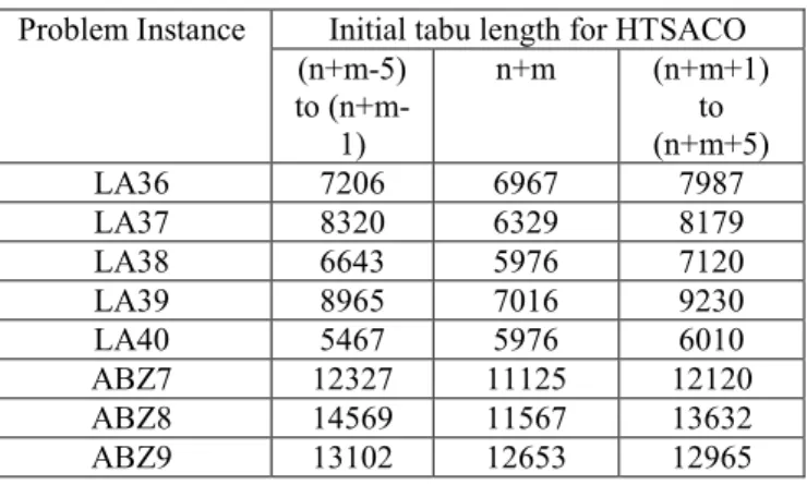
Table 4 shows the number of iterations required to reach the lower bound values by HTSACO for different values of the initial length of the tabu list. The values of ACO parameters are mentioned earlier in this section. The column 2 gives the average number of iterations required for optimal or the lower bound value with the initial tabu length between
n+m-5 and n+m-1. The column 3 gives the number of iterations required, when the length of initial tabu list is n+m. The column 4 gives the average number of iterations with the initial tabu lengths between n+m+1 and n+m+5. From the table 4, we understand that better results can be produced by setting the initial tabu length value as n+m.
Table 4
Table 4. Number of iterations required to reach LB value for different values for initial length of the tabu list
Problem Instance Initial tabu length for HTSACO (n+m-5)
to (n+m-1)
n+m (n+m+1) to (n+m+5)
LA36 7206 6967 7987
LA37 8320 6329 8179
LA38 6643 5976 7120
LA39 8965 7016 9230
LA40 5467 5976 6010
ABZ7 12327 11125 12120
ABZ8 14569 11567 13632
ABZ9 13102 12653 12965
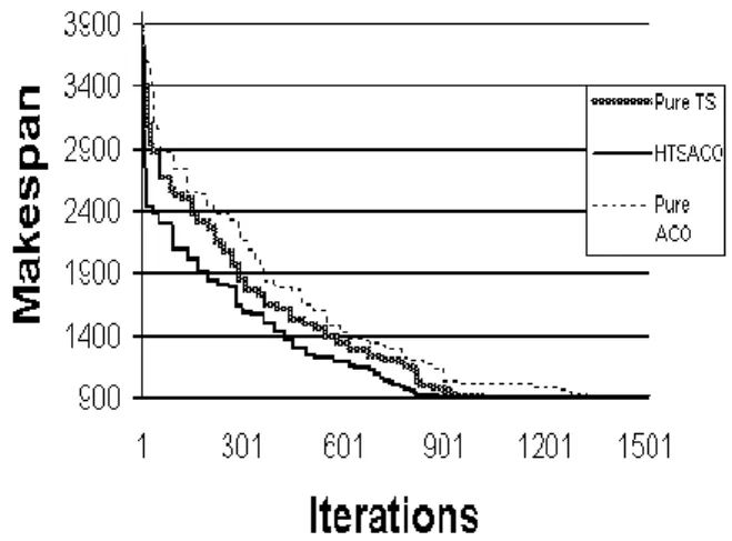
Typical runs of the problem LA20 is also illustrated in the figures 4 which give the results of comparisons of the iterations with the best makespan values produced from pure TS, pure ACO and HTSACO. It is clear from the figure 4 that Probl
em
n M Total Opera tions
Pure TS
Pure ACO HTS ACO CPU Sec LB value CPU Sec LB value CPU Sec LB value FT06 6 6 36 2(55) 4(55) 2(55) FT10 10 10 100 516(94
2)
642(956) 459(9 30) LA0
1
10 5 50 58(666) 94(666) 40(66 6) LA0
6
15 5 75 114(92 6)
145(926) 87(92 6) LA1
1
20 5 100 132(12 22)
168(1234) 98(12 22) LA1
6
10 10 100 164(94 6)
217(952) 150(9 45) LA2
0
10 10 100 202(90 2)
267(906) 178(9 02) LA2
1
15 10 150 1146(1 076) 1355(1122 ) 987(1 046) LA2 6
20 10 200 2143(1 256)
25391264) 1836( 1221) LA3
1
30 10 300 3578(1 812) 4154(1854 ) 2949( 1791) LA3 6
15 15 225 2962(1 296) 3978(1312 ) 2533( 1272) ABZ 5
10 10 100 4135(1 242) 5834(1274 ) 3124( 1234) ABZ 6
10 10 100 4563(9 52)
6862(984) 3897( 947) ABZ
7
15 20 300 6645(6 76) 11246(712 ) 5780( 662) ORB 1
10 10 100 5523(1 072) 9758(1262 ) 4594( 1067) ORB 2
10 10 100 6387(9 20)
10076(964 )
Volume 2 - Issue 6, June 2015
24 the performance of hybrid version HTSACO is better when compared with the methods of TS and ACO without hybridization.
Figure 4. Comparison of makespan Vs Iterations
7. Conclusion
This paper has presented the application of the tabu search with the ant colony optimization to solve the job shop scheduling problems. The goal of the work was to gain some insight into the influence of dynamic tabu length strategies in the tabu search and the pheromone trail in the ant colony optimization. The pheromone trial level between the operations of one neighbor and the time of operations of that neighbor seem to play an important role on the construction of the good solutions. The tabu length was also changed dynamically during the construction of the solution. The ant colony optimization method of selecting the neighborhood solution and the dynamic tabu length strategies were used to prevent the neighbors which keep the solution in local minima and also used to avoid cycling. The performance tests were carried out by using the proposed method with well known benchmark problems and the results of the proposed method were compared with the results of the other competing algorithms.
References:
[1] Glover F (1986) “Future Paths for Integer Programming and Links to Artificial Intelligence”, Computers and Operations Research, Vol. 13, pp. 533-549.
[2] Dorigo M, Maniezzo V, Colorni A (1996) “The Ant System: Optimization by a colony of cooperating agents”,
IEEE Trans. Systems, Man, Cybernetics, Vol. 26, no.2, pp.29-41.
[3] Dorigo M, Gambardella L.M. (1997) “Ant colony System: A Cooperative Learning Approach to the Travelling Salesman Problem”, IEEE Trans. On Evolutionary Computation, Vol.1, no.1, pp. 53-66.
[4] Glover F, (1989) “Tabu Search – Part I”, ORSA Journal on Computing, Vol. 1, pp. 190-206.
[5] Glover F, (1990) “Tabu Search – Part II”, ORSA Journal on Computing, Vol. 2, pp. 4-32.
[6] Ferdinando Pezzella, Emanuela Merelli (2000) “A Tabu Search Method guided by Shifting Bottleneck for the Job Shop Scheduling Problem”, European Journal of Operational Research, Elsevier, Vol. 120, pp. 297-310. [7] Calderia J.P., Melicio F, Rosa A (2004) “Using a Hybrid Evolutionary-Taboo Algorithm to solve Job Shop Problem”,
ACM Symposium on Applied Computing, pp. 1446-1451. [8] Eugeniusz Nowicki, Czeslaw Smutnicki (2005) “An Advanced Tabu Search Algorithm for the Job Shop Problem”, Journal of Scheduling, Vol. 8, pp.145-159. [9] Applegate D, Cook W (1991) “Acomputational Study of the Job-Shop Scheduling Problem”, ORSA Journal on Computing, Vol. 3, pp. 149-156.
[10] Ponnambalam S.G., Aravindan P., Rajesh S.V. (2000) “A Tabu Search Algorithm for Job Shop Scheduling”,
International Journal of Advance Manufacturing Technology, Vol. 16, pp. 765–771.
[11] VinmH cius Amaral Armentano, Cintia Rigao Scrich (2004) “Tabu search for minimizing total tardiness in a job shop”, International Journal of Production Economics, Vol. 63, pp.131-140.
[12] Christian Blum, Michael Samples, (2004) “An Ant Colony Optimizatino Algorithm for Shop Scheduling Problems”, Journal of Mathematical Modeling and Algorithms, Kluwer Academic Publishers, Netherlands, Vol. 3, pp. 285-308.
[13] Ventresca M, Ombuki B.M. (2004) “Ant Colony Optimization for Job Shop Scheduling Problem”, Technical Report #CS-04-04, Brock University, Canada.
[14] Jun Zhang, Xiaomin Hu, Tan X, Zhong J.H., and Huang Q (2006) “Implementation of an Ant Colony Optimization technique for job shop scheduling problem”, Transactions of the Institute of Measurement and Control, Vol. 28, No.1, pp.93-108.
[15] Hertz A, de Werra D (1991) “The Tabu Search Metaheuristic: How We Used It”, Annals of Mathematics and Artificial Intelligence, Vol.1, pp. 111-121.
[16] Dorigo M, Maniezzo V, Colorni A (1991) “The ant system: an autocatalytic optimizing process”, Technical Report TR91-016, Politecnico di Milano.