Efficient tuning in supervised machine learning

(1)

Cover Page

The handle

http://hdl.handle.net/1887/22055

holds various files of this Leiden University

dissertation.

Author: Koch, Patrick

(2)

Efficient Tuning in Supervised Machine Learning

Proefschrift

ter verkrijging van

de graad van Doctor aan de Universiteit Leiden, op gezag van Rector Magnificus prof.mr. C.J.J.M. Stolker,

volgens besluit van het College voor Promoties te verdedigen op dinsdag 29 oktober 2013

klokke 13:45 uur

door

Patrick Koch

geboren te Lippstadt

(3)

Promotiecommissie

Promotor: Prof. Dr. T.H.W. B¨ack

Prof. Dr. W. Konen (Cologne University of Applied Sciences) Chairman: Prof. Dr. J.N. Kok

Overige leden: Prof. Dr. J. Branke (University of Warwick) Dr. W.A. Kosters

Dr. M.T.M. Emmerich

This work was partially supported by the Bundesministerium f¨ur Bildung und Forschung (BMBF)

under the grant “SOMA” (FKZ 17N1009), by the Kind-Steinm¨uller-Stiftung, and by the Cologne

University of Applied Sciences under the research focus grant COSA.

Cover artwork: Keith Peters

(4)

(5)

(6)

Chapter 1 Introduction

The tuning of learning algorithm parameters has become more and more important during

the last years. With the fast growth of computational power and available memory databases have grown dramatically. This is very challenging for the tuning of parameters arising in

machine learning, since the training can become very time-consuming for large datasets. For this reason efficient tuning methods are required, which are able to improve the predictions of

the learning algorithms. In this thesis we incorporate model-assisted optimization techniques, for performing efficient optimization on noisy datasets with very limited budgets.

Under this umbrella we also combine learning algorithms with methods for feature construction and selection. We propose to integrate a variety of elements into the learning

process. E.g., can tuning be helpful in learning tasks like time series regression using state-of-the-art machine learning algorithms? Are statistical methods capable to reduce noise effects?

Can surrogate models like Kriging learn a reasonable mapping of the parameter landscape to the quality measures, or are they deteriorated by disturbing factors? Summarizing all

these parts, we analyze if superior learning algorithms can be created, with a special focus on efficient runtimes.

Besides the advantages of systematic tuning approaches, we also highlight possible obstacles and issues of tuning. Different tuning methods are compared and the impact

of their features are exposed. It is a goal of this work to give users insights into applying state-of-the-art learning algorithms profitably in practice.

1.1 Motivation

Learning is the art of acquiring knowledge. Because nature and its processes can be very

complex, machines are often used to filter information and help humans in understanding the behaviour of such processes. Learning can be performed in many different ways: one

possibility is to learn from experience, thus gaining knowledge by self-learning or trial-and-error. Another option is to gain knowledge by learning from a teacher. In that case

(9)

4 1. Introduction

calledsupervised learning.

Many different learning algorithms exist, each being able to perform tasks like

classification or regression. Although these algorithms very often perform well in practice, they also have certain parameters, which need to be set carefully to get reasonable results. A

solution can be to use global optimization for minimizing the empiricial risk (or maximizing the performance of the learning algorithm). But as the evaluation of a learning algorithm

includes a complete model training and prediction of unseen test patterns, the optimization

can become expensive for larger datasets. Under such circumstances the question remains, whether the optimization can be performed within a feasible amount of time.

Supervised learning comprises the learning of a concept from labeled data [2, 42, 78, 77].

It has been studied intensively in the 20th century and today probably belongs to the most important research areas in Artificial Intelligence (AI) [208]. In other disciplines as

computer science, supervised learning is also sometimes referred to as pattern recognition [21]. Supervised learning especially received a boost with the increase in computational power

at the end of the 20th century. Buzzwords like “big data mining” have become popular in economy and industry. Learning from data usually includes a complicated process comprising

the choice of a suitable learning algorithm and special pre- and post-processing operators. Here careful decisions must be made, which appears to be even harder, when very little

domain knowledge is available for the task. Additionally, noise in the data causes a further blurring of the concept to be learned. Under such circumstances it is obvious, that finding

good settings for learning algorithms becomes difficult. As a possible solution, state-of-the-art optimization heuristics can be incorporated, which can help users defining better learning

processes. A decision support system which compares chains of operators and delivers the best combination in the end can help to solve this task.

For creating such a decision support system, we have to find out how learning is performed. The learning task in machine learning (ML) is very similar to learning of humans:

a ML concept or model is usually generated by learning from examples — the training data. Afterwards, a learning algorithm can be applied to unseen data (unbiased evaluation or

prediction) and if desired, it can then be refined by humans in a stepwise manner. Learning the target concept by using labeled information seems to be very attractive, because

machines can process information very quickly and can repeat the learning as often as needed. However, when a good input-output mapping is difficult to obtain, because many

data points have to be processed, the refinement process can be very time-consuming and humans tend to bias personal favourite choices. Then, instead of this human intervention

other approaches promise to be more systematic. These processes are known asmodel

optimization or model tuning. Here optimization algorithms are considered, which test

different configurations of learning algorithms, and combinations of pre-processing methods.

(10)

1.2. Survey 5

of its usability and effectiveness. In general, learning algorithms are only helpful when they

do not have any biases to specific data and the time required to create them is acceptable. Model optimization is often not incorporated in practice, because it is too

• time-consuming, or

• error-prone to biases and wrong model assumptions caused by high noise levels.

These two topics are important points for all learning algorithms and we will address both issues in this thesis. It has to be analyzed how tuning of learning algorithms can be justified

against no tuning at all, or a simple hand-tuning of learning algorithms.

1.2 Survey

This thesis is structured as follows: methods for ML and preliminaries of stochastic optimization are given in Chapter 2.

In Chapter 3 we add techniques for feature processing to the learning process and show

how beneficial they are for the prediction accuracy of learning algorithms.

Learning algorithms are systematically coupled with optimization techniques in Chapter 4.

The demand for parameter tuning is motivated here, by comparing baseline tuning algorithms with state-of-the-art optimization techniques. As a new field of research we apply

model-assisted optimization to improve the performance of learning algorithms on noisy data with very restrictive budgets.

In Chapter 5 we especially focus on the efficiency of the tuning, which is one important aspect to make ML tuning ready-to-use for real-world applications. We apply sub-sampling

techniques, combined with special noise handling strategies for surrogate models, and use repeated evaluations to handle noisy evaluations by the optimal computing budget allocation

(OCBA).

The quality of the fit of parameter spaces is analyzed in Chapter 6. This chapter is

especially interesting to reveal the weaknesses of certain surrogate models. Here, we show, that high noise levels can deteriorate the fitness landscapes of these models, requiring

additional noise handling approaches to avoid misleading settings during the tuning. A new, different perspective of tuning in ML is described in Chapter 7, where ML tuning

is transferred to a multi-criteria task. Although multi-criteria optimization has been analyzed for engineering applications earlier, it has never been considered for ML optimization.

(11)

(12)

Chapter 2 Methods

In this chapter we introduce methods and operators which are necessary elements for

the experiments in this thesis. We start with a brief introduction to machine learning in Sec. 2.1 and proceed with more detailed descriptions of feature selection and feature

construction in Sec. 2.2 and Sec. 2.3 respectively. Finally we give an overview about methods of Computational Intelligence in Sec. 2.4 and present the state-of-the-art of model-assisted

optimization in Sec. 2.5.

2.1 Machine learning

Machine learning is the process of gaining knowledge using computers without programming

the knowledge explicitly. In general two different types of learning can be distinguished:

• Supervised learning: direct training feedback is available in form of examples for which the output is known.

• Unsupervised learning: training is indirectly done, e.g., by performing self-learning methods such as trial-and-error.

In this thesis the focus lies on supervised learning, nevertheless parts of the research can also be applied to unsupervised learning.

2.1.1 Supervised learning

Supervised learning belongs to the most widely researched fields in artificial intelligence.

The goal is to train a computer model which is capable to predict new data.

In supervised learning a mapping from input data to a target variable is trained by using examples. The target variable can be represented by discrete values (or classes), whereas we

call this a classification task. The target can also be a continuous variable, and in this case

we call the learning taskregression. As a third special case we will also investigate learning

(13)

8 2. Methods

2.1.1.1 Learning from data

The data for machine learning is usually stored inside a file or a database. The entries of

this file or database are calledinstances orpatterns. A dataset for ML can be written as a

sequence of pairsD = (~x1, y1),(~x2, y2), . . . ,(~xn, yn), consisting of input data or feature

vectors~x(i) _{and their corresponding outputs}_y(i)_{. Each input}_~_x(i)_{consists of}_N _attributes

describing the characteristics of the instance. Later we will also denote the input attributes as features. In supervised learning, the algorithms require outputs to train a prediction

model. E.g., in classification they require at least one instance of each class in the training

data. Forclassificationtasks the target variables yi are defined by a finite set with a fixed

number of elements, the corresponding classes. Inregression, the valuesyi are defined by a

continuous space, e.g.yi ⊆R.

Feature 1 Feature 2

x

x x

x

Class 1 Class 2

x

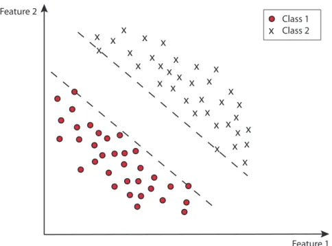
Figure 2.1:Linear separability of a binary classification problem. The figure shows data points (instances

(14)

2.1. Machine learning 9

Figure 2.2:Poisonous or edible? The mushroom Amanita muscaria or “Fly agaric toadstool”. Picture by

Tony Wills, License: Creative Commons Attribution 3.0 Unported

2.1.1.2 Classification

In classification we are interested in finding a separating hyperplane in theN-dimensional

feature space, which is able to classify each pattern to its belonging target label. E.g., in

Fig. 2.1 a two-class example is shown, where the class patterns are displayed as crosses and circles. The two dashed lines represent possible margins for each class. Every hyperplane

between these two margin lines can separate the class patterns by classifying all points to the left side as circles and the points on the right side as crosses. An early learning algorithm

that makes use of a separating hyperplane is the perceptron invented by Rosenblatt [207], which later led to the concept of Artificial Neural Networks (ANN) [109].

An intuitive example for classification is to classify mushrooms. Mushrooms can be

eitheredible orpoisonous. If we write down examples for mushrooms, including attributes

like colour, size, points, etc., and denote the class label for each example, we can train a

learning algorithm which is capable to classify mushrooms. The learning algorithm would use the known examples for predicting new unknown examples into edible or poisonous. Of

course, the probability of classifying new samples, increases, if a certain number of training patterns is available, and under the assumption that the training data is correct.

2.1.1.3 Regression

In classification the output was considered as a discrete and finite variable. However, in

many applications it is desired to predict numerical values like real numbers, e.g., to predict

sensor measurements in an engineering process. In this case we performregression, instead

of classification.

Although regression is a different approach, real-valued output functions can also be

(15)

10 2. Methods

model for regression is thelinear model:

yi=w0+w1xi,1+w2xi,2+. . .+wNxi,N +εi (2.1)

The linear model predicts the target by learning the optimal weighted sum of the input

features. The weights w~ = w1, ..., wN are determined by an optimization procedure

minimizing the error of the training set. The weight w0 is just an offset and the term

εi acts as slack variable. The weights for the model are based on the training data and

can be determined by minimizing a loss function like the mean squared error (MSE). For

predictions~yˆand real observations ~y the MSE for a training set of sizen is defined as

follows:

1

n

X

i=1

(ˆyi−yi)2 (2.2)

In practice often the root mean squared error is considered:

v u u t

1

n

X

i=1

(ˆyi−yi)2 (2.3)

It is possible to use interpretable models like the linear model in Eq. 2.1 to reveal feature importance. The disadvantage is that linear models are limited to easier data. More powerful

models with the opportunity for interpretability are, e.g., multivariate regression splines

(MARS) [87], or other techniques for symbolic regression like Genetic Programming [158].

2.1.1.4 Time series analysis

In many engineering applications data is dependent on atime label, which represents the

information when the data was recorded. In history time series have been known at least since the 10th century (cf. Fig. 2.3). A well-known example of a time series application is

the prediction of stock market prices. Here, the prices have an additional time information.

Thus, the price of a stock is defined by its value at timet. Outgoing from timetthe price of

a stock can rise (hausse) or fall (baisse). It is important to note, that the price in the future

t+kis often dependent on time tand also on outer events from the environment which

occurred in the period fromt+kup to some earlier timet−`. Of course the predictability

in the future is usually limited to a certaink, because the stock market situation of today

will only have a marginal influence to the situation in the next day or hour. But it is assumed

that the time series can be predicted in the future up to a certaink. The learning algorithms

can gain from adding influences from outside, e.g., actual news. The price of the stock can change according to the information given in such additional reports. The other assumption

in time series analysis isautoregression, e.g., that the price will depend on the change of

earlier values. This corresponds with time series like weather forecasts, where it can be

(16)

Figure 2.3: The figure shows a historic drawing of an early time series in the 10th century. Drawing

found in [170, 241].

output values of time series data are correlated to a) the values of the time in the past and b) changes or actions in the underlying domain.

Usually a time series is recorded as a discrete stochastic process from time T = 0tot:

(~x(0), y(0)),(~x(1), y(1)), . . . ,(~x(t), y(t)) (2.4)

In the simplest case the output is equal to the input ~x(i) ₌_y(i)_{, for all} _i_{= 0}_{, . . . , t}_.

Then the time series can be simply written as

~

y=y(0), y(1), . . . , y(t) (2.5)

The time series in Eq. Eq. 2.5 is called a univariate time series. Here, the time series is

solely defined by the probabilistic structure (the mean and variance) of the samples ofy. In

this case, classical time series analysis methods like ARIMA or GARCH processes can be

used [31]. However, these methods are limited, because they are suited for linear processes and also assume a certain autocorrelation of the target. Instead, regression techniques from

ML can be applied, to detect more difficult structures in the time series.

Today there is a large demand for analyzing multivariate time series. Here, at any time

pointt more than one variable is recorded. All variables have a certain influence on the

target variable, which is in general unknown for arbitrary tasks.

2.1.2 Learning algorithms

The state-of-the-art in ML is difficult to grasp. Many algorithms exist, capable for many purposes, so that a certain favourite can hardly be named here. However, at least two

(17)

12 2. Methods

by setting their parameters: random forest [26] as representative of decision tree-based

methods and Support Vector Machines (SVMs) [245]. In this section we define the learning algorithms, a more detailed description on the underlying hyperparameters is then given in

Sec. 4.2.

2.1.2.1 Random forest

Random forest (RF) [26] is a learning algorithm based on classification and regression trees

(CART) [28]. RF uses an ensemble of decision or regression trees for the prediction. For ensemble methods we use a number of independent learning algorithms, which are later

combined by an aggregation procedure. The goal is to get a better result using the ensemble, compared with possible weak results of single learning algorithms itself [102]. E.g., the CART

approach by Breiman [28] has weaknesses, because the single trees are prone to overfitting. With the aggregation of many trees in an ensemble, such weaknesses of single learning

algorithms are compensated. The most prominent two methods for ensemble learning are boosting [212] and bagging [24], which are described in the following sections.

RF uses the bagging approach (see Sec. 2.1.2.2) to create the tree ensemble. Additionally,

a random feature selection for each node of the trees is taken from Ho [112, 113] and Amit and Geman [3]. These advantages of tree learners leads to a very robust algorithm, which is

very stable to issues like overfitting or noise in the data.

Although RF is almost parameter-free, and already works well with default settings, it is sometimes advantageous, to optimize certain parameters [218]. As important parameters

for RF, the number of trees (ntree) in the ensemble can be mentioned [232], as well as the

number of splits performed in each tree node (mtry). Instead of performing a tuning of

mtry, Liaw and Wiener [166] suggest the following defaults based on the number of features

p:

mtrydefault =

(

max(bp₃c,1), if task is regression

√

p, else (2.6)

It has to be noted, that this formula is only a rule of thumb. In our experiments we will

also see advantages of tuningmtry. Other tuning options include the computation times of

the algorithm, e.g., by setting thesampsize parameter (sample size used for the RF trees).

2.1.2.2 Ensemble approaches Bagging

Bagging [24] is an acronym forbootstrap aggregating, where bootstrapping refers to a

resampling method [67]. In bootstrappingk learning or training subsets of the training set

sizenare drawn repeatedly random with replacement from the complete training data. An

(18)

subset. For the prediction all models in the ensemble predict the test pattern. For the final

output, thekpredicted outputs of the models areaggregated by an aggregation function.

As aggregation function, e.g., majority voting [190] can be used, or one can take the mean

of all ensemble learners in regression.

Boosting

Boosting was presented by Schapire [211] and has been later improved by Freund and Schapire [86]. In boosting, the complete training data is used for the training, but a weight

is assigned for each training pattern. At first the weights are uniformly distributed for all patterns, and then updated during the algorithm run. The weighting scheme is defined by

variableswt(i), which denote the weight of pattern~x(i) in iterationt of the algorithm. In

each iteration training patterns are sampled usingwt(i)as probability distribution for the

sampling with replacement. After having drawn the training data according to the weighting scheme all ensemble learners are trained using these sets. Then the weights are updated,

assigning a smaller weight for correctly predicted patterns, and an increased weight for wrongly predicted patterns respectively. In the next round the sampling and training is

applied again until a termination condition holds. Possible termination criteria are, e.g., a limited number of model trainings or a time limit.

When the target variable has a certain number of wrong values, the prediction accuracy degenerates for boosting, as shown by Dietterich [58]. For this reason bagging is used within

RF.

2.1.2.3 Support Vector Machines

Support Vector Machines (SVMs) have been originally introduced as learning algorithms

for binary classification and regression tasks [215], but they can also be used to solve multi-class problems, e.g., by incorporating multiple “one-against-all classifiers” (see [23]

for a comprehensive overview).

Our main intention for using SVMs — besides that SVMs are known as a powerful ML

tool — is that SVMs tend to be very sensitive to parameter settings, which makes them interesting for parameter tuning tasks. In binary classification, SVMs seek the maximal

margin classifier, which best separates the two classes. In the simplest case this means to search for the optimal separating hyperplane by minimizing the empirical risk. However, if

SVMs could only classify separable data, the applicability would be very limited, since most real-world problems are not linearly separable. Therefore, SVMs perform classification with

the following extensions:

(19)

higher-14 2. Methods

dimensional space using a kernel function

K(X, ~~ Z) =hφ(X~)·φ(Z~)i (2.7)

where φ defines a mapping from the input space. A simple example for such a

transformation is to calculate the monomials of the input features and to consider

them for the mapping. The kernel function denotes the similarity of two observations

~

X and Z~. Because the kernel function can be interpreted as a dot product in a

high-dimensional space, the computation is feasible also for very high dimensions. When the patterns cannot be separated by a linear classifier in the original feature

space, this can be still possible in the kernel-induced feature space. The kernel function can be defined anew for each task, or pre-defined kernel functions can be chosen. It is

important that kernel functions fulfill the Mercer theorem [180], as they have to be positive definite and symmetric (PSD property).

The most frequently used kernel functions for SVMs include the following functions:

– Linear

K(X, ~~ Z) =h_{X, ~}~ _Z_i _(2.8)

– Polynomial kernel:

K(X, ~~ Z) =hX, ~~ Zid _(2.9)

– Radial basis function (RBF):

K(X, ~~ Z) = exp −||X~ −Z~|| 2

2γ2

!

(2.10)

where γanddare parameters for the corresponding kernel functions.

(2) Regularized risk minimization: If some observations are still not classified correct in the kernel-induced feature space, SVMs can make use of the soft-margin concept

by Cortes and Vapnik [51]. In soft-margin SVMs a regularization term is introduced, which penalizes wrongly classified patterns. Making this more rigorous, we can write

the optimal SVMs classification model in the unconstrained dual form, denotingH as

the reproducing kernel Hilbert space for the kernel functionK(·,·), in the following

optimization problem:

ˆ

F = arg inf

F∈H,b∈R

||F||2

H+C n

X

i=1

L(Yi, F(X~i) +b) (2.11)

(20)

−4 −3 −2 −1 0 1 2

0.2

0.4

0.6

0.8

1.0

Input space x

Attribute 1

Attr

ib

ute 2

● _●

●

● ●

−4 −3 −2 −1 0 1 2

−2

−1

0

1

2

3

4

Feature space φ(x)

Feature space 1

F

eature space 2

●

● ●

Figure 2.4:Mapping from input to feature space via kernel functionφ. Before the mapping, the data is

not separable, after the mapping a linear classifier can separate the class patterns.

of binary classification we would discretize the real-valued output of Fˆ by mapping it

to{−1,1}. The first term is called a smoothness penalty using a regulariser|| · ||2

H,

whereH is the Hilbert space of functions defined over the input domain [52, p. 40].

The 2-norm can be used to penalize non-smooth functions. The second term measures

the closeness of our predictions to the true outputs by means of a loss function. In

classification, we usually select the hinge lossL(Y, t) =Lh(Y, t) = max(0,1−Y t)

for an intended output t=±1and a classifier scoreY. For regression we often set

L(Y, t) = L(Y, t) = max(0,|Y −t| −) to the -insensitive loss. The hinge loss

is a convex, upper surrogate loss for the 0/1-loss (which is of primary interest, but

algorithmically intractable), while L provides the estimation of the median of Y

givenX~. Both losses lead to quadratic programming problems for Eq. 2.11, which can

be solved efficiently, and the non-differentiability of these two loss functions further

provides for sparse solutions [43]. The two terms are balanced by the parameterC,

sometimes also referred to asCost. In recent SVM implementations, a value ofC= 1

is taken as default, equally weighting loss function and smoothness penalty.1

The optimal kernel function may vary depending on the data. Without having any prior knowledge, the RBF kernel works well in most cases, presuming that the kernel parameters

are set to good values. Of course the RBF and polynomial kernel functions are more complex

(21)

16 2. Methods

and are able to classify non-separable data better than a linear kernel. But as a drawback

they are more expensive to compute.

In regression, usually the Support Vector Regression (SVR) approach of Drucker et

al.[63] is applied. For more information about SVR the interested reader is referred to the

tutorial of Smola and Schlkopf [228]. For simplicity we do not distinguish between SVR and SVM in this thesis, but indicate which method is used where it is necessary.

A recent overview about the state-of-the-art in learning with kernels has been given by

Signoretto and Suykens [221].

2.1.3 Generalization and benchmarking

In ML experiments a dataset

D=(~x(1), y(1)),(~x(2), y(2)), . . . ,(~x(m), y(m)) (2.12)

consists ofmexamples or instances and the corresponding output, e.g., a class label or real

value.

If all training patterns in the data D are consistent, the optimal learning algorithm

would always give the correct answer for every new example. Of course this is a very strong assumption for most datasets, and even when this holds, it remains unclear, if the learning

algorithm also behaves optimal on future instances. Thus, in practice approximations of

this optimal model are computed. In order to compare these models, we have to define a procedure, under which we can measure the model quality. This is known as benchmarking

of ML algorithms.

Benchmarking of learning algorithms belongs to one of the most controversely discussed

topics in ML and statistics: Hothorn et al. [116] describe a theoretical framework for

benchmarking. Eugster and Leisch [73] and Eugster et al. [72] present techniques for

visualizing benchmark results. Hornik and Meyer [114] propose to use consensus rankings

for benchmarking ML algorithms. Bischlet al.[20] discuss resampling strategies for tuning

of learning algorithms and describe common pitfalls and advantages of the methods. In experiments it is important to take into account statistical analyses to provide

sound results. Public benchmark sets like the UCI repository [84] are available and can be downloaded from the internet. There are at least two reasons for using public datasets:

evaluation with public datasets makes the results of algorithms reproducible, because every researcher is able to test his method on these datasets. Second, researchers can help in

improving methods when they are applied to common datasets.

However, we also think that public benchmark sets alone might be not sufficient for a sound benchmarking of algorithms and can result in overfitting to certain benchmark

repositories itself. Besides that, the motivation behind developing new algorithms is to solve new problems. Here, public benchmark datasets might be too restrictive. Instead we think

(22)

be made. Learning algorithms are also thought to find hidden structures in unknown data,

and if benchmarks are too restrictive, it can happen that in the sequel the development of learning algorithms stagnates.

In the following paragraphs, we introduce methods for evaluating ML algorithms. A

desirable property of ML algorithms is, that they can generalize well and perform good on other unseen data. Therefore, special resampling strategies exist, which play a key role for

all experiments made in this thesis.

2.1.3.1 Sampling strategies

ML models should be well generalizing, to learn a model for the dataset. The learning

algorithm should be able to generate predictions for new patterns ~x(o) with a maximal

accuracy. In this section sampling methods are proposed, which aim at estimating the

generalization error. These sampling methods include:

• Random sampling (holdout set)

• k-fold cross-validation

• Leave-one out cross-validation

• Sub-sampling

• Stratified sampling

Random sampling

For training and testing purposes the datasetDis usually split randomly into disjoint

subsets

L ⊂ D (2.13)

and

T ⊂ D (2.14)

withL ∪ T =D. Now each learning algorithm can be trained on the training dataL, while

it can be evaluated on test data T. This accuracy estimation method is called holdout

method, because the patterns of setT are held out during training.

Cross-validation

Another method for estimating the generalization performance is the k-fold cross

(23)

18 2. Methods

{1, . . . , k}a prediction model is trained, predicting the remaining patterns

D(j) =D\D(i) (2.15)

Finally the errors of each learned model can be aggregated, e.g., by taking the mean of the errors.

Leave-one out cross-validation

Leave-one out cross-validation (LOOCV) is a special case of k-fold cross-validation,

where the numberk is equal to the number of patterns of the dataset (k=|D|). LOOCV

certainly gives the best estimate of the real generalization performance. Unfortunately LOOCV belongs to the most expensive methods to evaluate learning algorithms, and for

this reason it is not well suited when many models must be built, as is the case in parameter tuning of learning algorithms.

Sub-sampling

Normally all available training patterns in the data setDare used for training. Sometimes

Dtends to be very large, and the training takes a lot of time. Additionally, outliers and

redundant patterns can be misleading for learning the concept. In such cases, we can perform a training using only small subsets (subsamples) of the available training data. This sampling

strategy is calledsub-sampling and is very effective, when it is repeatedly performed, e.g.,

in a tuning process.

Learning with reduced training set sizes can give remarkable speed-ups for the

model-building process, which is the main reason for using it in practice. Last [161] proposes partial learning by projective sampling to estimate the optimal training set size. For Artificial

Neural Networks [38] and Support Vector Machines [220], intelligent sub-sampling near the decision boundary helps to speed-up the training process without loss of accuracy. In

many studies it was observed that training with smaller sets does not necessarily lead to worse generalizing prediction models. Instead, the complexity of the trained models can be

reduced as shown by Oates and Jensen [187] and Provostet al.[196]. Some people think

that simpler hypotheses should be preferred, which was constituted in Occam’s razor [22].

Stratified sampling

When performing sub-sampling, it can happen that the training set sizes tend to be very small, which is especially the case for smaller datasets. Another situation where this issue can

occur is data, where the classes are imbalanced. This can lead to training sets, where whole classes are missing. Stratified sampling [186] is a sampling strategy for classification to solve

(24)

2.2. Feature selection 19

at random, but draws them from eachstratum or class. By doing this the distribution of

the class probabilities remains unchanged.

2.2 Feature selection

Feature processing probably belongs to one of the most important steps for obtaining better prediction models. In this section we introduce various methods for feature subset selection,

which are capable to form better feature starting sets. It is shown in [255], that although

the dataset itself does not contain more information with a reduced feature subset, the selection can be beneficial for the generalization performance. Although this does not seem

to be very logical at first sight, the reason is that unimportant features in the dataset can deteriorate results. With a better feature set, noise is reduced in the data and a better

classification or regression model can be obtained. Due to the high importance of feature selection, we include hyperparameters of feature processing algorithms in the tuning, in

order to generate more powerful learning algorithms.

Feature subset selection can be of large importance, because the model benefits from a reduced feature subset, where non-informative features are excluded. Guyon and Elliseeff [101]

present a comprehensive overview about this topic. In general we can distinguish between three different types of feature selection:

• Filter approaches give rankings of the features without training a learning algorithm

• Wrapper approaches return feature subsets by applying a specific learning algorithm in an iterated manner

• Embedded methods are integrated into some learning algorithms, which enables off-the-shelf feature rankings

All approaches have their advantages and disadvantages, which are briefly described in the following sections.

2.2.1 Filter approaches

Feature selection using filter methods is solely based on criteria without requiring to build and to evaluate a specific learning algorithm. For this reason these methods are very attractive,

because building learning algorithms for large-scale data can become computationally expensive, and filter methods always provide a quick alternative for measuring the information

(25)

20 2. Methods

2.2.1.1 Correlation-based filtering

A well-known measure to determine the similarity of two variables is the linear correlation.

For two variables~xand~y the correlation is defined by

ρ=

Pm

i=1(xi−µ(xi))·(yi−µ(yi))

Pm

i=1

p

(xi−µ(xi))2·

p

(yi−µ(yi))2

(2.16)

whereµ(xi)andµ(yi)are the mean values of variable~xi and~yi respectively.

The output ρ lies in the range between −1 and 1, indicating a negative or positive

correlation between the two variables.

2.2.1.2 Entropy and information gain

Instead of the linear correlation measure, often the entropy is been used for measuring the

information content of a variable~x. The entropy is defined by

H(~x) =

m

X

i=1

P rob(xi) log(P rob(1/xi)) (2.17)

Now we can define the following quantity for measuring the entropy of~xafter ~y was

observed:

H(~x|~y) =−

m

X

j=1

P rob(yj) m

X

i=1

P rob(xi|yj) log2(P rob(xi|yj)) (2.18)

whereP rob(xi|yj)is the posterior probability of~xunder~y.

As an alternative to the entropy, Quinlan [197] introduced the information gain, which is based on the entropy and became popular as splitting rule in the C4.5 learning algorithm [197]:

IG(~x|~y) =H(x~)−H(~x|~y) (2.19)

2.2.1.3 Random forest importance

Random forest includes a method for ranking features, which is called random forest

importance (RFI). RFI cannot be classified as a filter approach, because it exhibits several

differences to the other approaches mentioned so far, but it is not a wrapper either. Instead

it can be categorized as anembedded method, because although RF is used for determining

a feature ranking, the ranking is ratherbuilt-in the learning algorithm [101]. For this reason

a prediction model has to be learned only once to obtain a feature ranking and not multiple

times like in wrapper approaches.

The advantage of the RFI method is that it can detect variable interactions, which the other filter approaches were not able to. The idea is as follows [27]: permute a variable or

feature by looking how much the prediction error increases when all other variables remain the same. Two measures are considered for the RFI:

(26)

2.2. Feature selection 21

• the mean decrease in Gini index [92] describing the node impurity measure [25, 169]

which is often used in tree-based classifiers.

These measures are obtained by performing the permutation test: When a certain feature

Vjis permuted, the out-of-bag (OOB) performance or the Gini index changes. The difference

between this performance and the prior performance is calculated for all trees. The average

of the tree values then describes the RFI measure for featureVj.

2.2.2 Wrapper approaches

In wrapper approaches the learning algorithm is used to perform a prediction of the task given a certain feature subset. In general words a search in the feature subset space is performed,

using the prediction error as objective function value to be minimized. Well-known examples are exhaustive search (which is NP-hard, making the runtime intractable in high dimensions

unlessP =N P), Genetic Algorithms or feature forward selection and backward elimination.

Kohavi and John [152] give a comprehensive survey of wrapper approaches. We describe

the most often used approaches in the following sections.

2.2.2.1 Feature forward selection

Feature forward selection is an iterative procedure where one feature is selected in the beginning. Using this single feature a model training is performed. After evaluating the

model, the accuracy on the evaluation set is taken as feature importance. In the first iteration

the algorithm would use all features to buildN prediction models. The feature with the

best prediction accuracy is then selected as most important feature. Outgoing from this

feature all other features are added and againN models are built. The procedure is iterated,

until no more improvement with adding new features can be made.

The disadvantages of the forward selection method are obvious: first, if the number of features of the dataset is large, many model trainings must be performed to obtain

a feature subset. This gets even more expensive, when a large fraction of the features is advantageous for the learning algorithm. Secondly, the method cannot detect complex

variable interactions. Let us assume that featuresV1andV2 together are perfectly suited

to predict the target variable. However, featureV1 andV2 both do not give any improved

prediction when considered exclusively. This means, that the method would converge and

both featuresV1 andV2 would never be added to the feature subset.

2.2.2.2 Genetic feature selection

Another heuristic for feature selection is the classical Genetic Algorithm (GA) [98]. A set

or population of binary strings of lengthN (corresponding to the number of features) is

initialized first. A ’1’ at positioniin the binary string indicates, that the feature is selected,

(27)

22 2. Methods

Note, that number of possible feature sets increases exponentially with the number

of available features/attributes (2N). For this reason a genetic search can become

computationally expensive. Another point is that empty feature sets must be avoided,

e.g., a string full of zeros would lead to crashes for most learning algorithms. Therefore in most implementations of genetic feature selection a parameter constant is added, denoting

the number of features to be used.

2.3 Feature construction

In this section we describe the creation of new features by performing specific transformations

or projections. We show how these transformations can be learned semi-automatically

providing only a set of basis functions. Although datasets sometimes already contain attributes which are good descriptors of the target, it can be helpful to derive new features

using the original attributes. These can beprojections or other transformations performed

on the data. Well-known data transformation methods are, e.g., the Principal Component

Analysis (PCA), or logarithmic and Fourier (spectral) transformations. Another possibility is

to calculate monomials of the input attributes of degreed.

In some cases features can be derived by recommendations of experts. However, this requires of course a detailed knowledge about the properties of the data. For this reason we

propose to use methods, which require only little knowledge, and which can be applied to most numeric datasets without any prior information. In Sec. 3.1 we show how user-based

feature construction can be combined with model-assisted tuning for improving prediction models. Another feature processing method which has received only little attention so

far is the Slow Feature Analysis. Combined with a simple classifier it can be used as a state-of-the-art learning algorithm, producing almost as good results as a SVM and RF, but

in much shorter time. Otherwise the main purpose is to use it as a pre-processing method for other learning algorithms. We applied SFA to a gesture recognition problem and achieved

remarkable results.

2.3.1 Principal Component Analysis

Principal Component Analysis (PCA) was firstly proposed by Pearson [189] and later formalized and named by Hotelling [115]. The goal of PCA is to find the directions in the

data which have the highest variance. It is a classical projection method for learning with reduced feature sets. PCA transforms the coordinate system by determining the maximum

variance of the input dimensions. PCA is helpful when attributes are correlated. In such cases PCA transformations can help to reduce the total number of features, without losing

too much information.

In the application of PCA, in a first step, the data is mean-centered. Afterwards, the

(28)

2.3. Feature construction 23

matrix to obtain the eigenvectors. Then, the eigenvectors are sorted in order of decreasing

eigenvalues. Note that the eigenvalues can represent the data, because they inherit the variances of the samples in the dataset. Eigenvalues are also often used in image calculations,

since transformations can easily be made when the structure is available. Now we can use them for reducing the number of features of the data. With fewer features based on the

largest eigenvalues of the covariance matrix we can often achieve better predictions for the task.

Formally PCA can be defined as follows: the covariance matrix of the data is denoted

byC~. Now the eigenvectors of this matrix are determined, and sorted in order of decreasing

eigenvalues. The matrix of the eigenvectors is written asU~. Now we simply calculate the

product ofU~ andC~:

~

Y =U~TC~ (2.20)

The output matrix Y~ comprises the transformed feature space, from which we can now

select the firstdrows, to reduce the originalm-dimensional feature set to d < mprincipal

component features. The more components are selected, the less variance of the data can

be observed in the transformed space. Because PCA is affected by scaling, all attributes are at first standardized to zero mean and unit variance. Instead of using PCA, sometimes the

Singular Value Decomposition (SVD) proposed by Golub and Van Loan [100] is considered,

since it is more robust in determining the eigenvectors, especially when the covariance matrix is singular.

The most relevant drawbacks of PCA and comparable methods are, that they are only

suited to make transformations of real-valued attributes. If discrete attributes are present in the data, PCA is not applicable any more. A frequently used approach is then to remove

these features from the dataset and to apply PCA only to the numerical part of the data. From our perspective PCA is a part of the learning process and therefore should be

also incorporated into the tuning. Although no direct parameter is required for PCA, the

number of featuresdto be selected from the transformed feature space, can be seen as a

hyperparameter.

2.3.2 Monomials

Monomials are products of attributes or features of degreed. Assume we have three features

denoted bya, b, cin the dataset. The set of all possible monomials of degree2would then

be

F :={a2, b2, c2, ab, ac, bc} (2.21)

It can be valuable to calculate such feature sets and use them instead of only the basis attributes. The reason is the higher-dimensional space the data is projected in. The main

(29)

24 2. Methods

expensive to calculate. For this reason monomials are usually only calculated for the most

important features. The importance of the features can be determined by using a feature ranking, e.g., through a filter, or by PCA through the level of variance of the principal

components.

2.3.3 Slow Feature Analysis

Slow Feature Analysis (SFA) is a learning algorithm from neuroscience which is capable

of learning unsupervised new features or “concepts” from time series. SFA was originally developed in context of unsupervised learning of learning invariances in the visual system

of vertebrates [252]. In [253] and [254] a detailed overview about the algorithm is given. Although SFA is inspired from neuroscience, it does not have the drawbacks of conventional

Artificial Neural Networks (ANNs) such as long training times or strong dependencies on initial conditions. Instead, SFA is fast in training and it has the potential to find hidden

features out of multidimensional signals, as shown by [16] for handwritten-digit recognition. SFA is optimally suited to construct features for time series signals. The original

SFA approach for time series analysis is defined as follows: For a (multivariate) time

series signal ~x(t) where t indicates time, find the set of real-valued output functions

g1(~x), g2(~x), ..., gM(~x), such that each output function

yj(t) =gj(~x(t)) (2.22)

minimally changes in time2_:

∆yj(t) =hy˙j2itis minimal (2.23)

The∆-value can be described by measuring the slowness of an output signal as the time

average of its squared derivative [254]. To exclude trivial solutions we add some constraints:

hyjit= 0(zero mean) (2.24)

hy_j2it= 1(unit variance) (2.25)

hykyjit= 0(decorrelation for k > j) (2.26)

The third equation is only relevant from the second slow signal on to prevent higher

signals from learning features already represented by slower signals.

For arbitrary functions this problem is difficult to solve, but SFA tries to find a solution

by expanding the input signal into a nonlinear function space by applying certain basis

functions, e.g., monomials of degree d. This expanded signal is sphered to fulfill the

2_h·i

(30)

2.3. Feature construction 25

constraints of Eq. 2.24, Eq. 2.25 and Eq. 2.26. Then SFA calculates the time derivative

of the sphered expanded signal and determines from its covariance matrix the normalized eigenvector with the smallest eigenvalue. Finally the sphered expanded signal is projected

(31)

26 2. Methods

Berkes [16] extended this approach to classify a set of handwritten digits. The main

idea of this extension is to create many small time series out of the class patterns: let us

assume that for aK-class problem each classcm∈ {c1, ..., cK}has gotNmpatterns. We

then reformulate the∆-objective function (2.23) for SFA with distinct indiceskandl as

the mean of the difference over all possible pairs:

∆(yj) =

1

npair

·

Nm

X

m=1

Nm

X

`=k+1

gj(p

(m)

k )−gj(p

(m)

` )

2

(2.27)

wherenpair denotes the total count of all pairs and p

(m)

k andp

(m)

l represent thek-th and

l-th class pattern of classm. The constraints defined by Eq. 2.24, Eq. 2.25 and Eq. 2.26 can

be reformulated then by substituting the average over time with the average over all patterns,

such that the learned functions have a zero mean, unit variance and are decorrelated [16].

As shown by Berkes [16], the(K−1)slowest SFA output signals are expected to have

a low intra-class variation, but usually a high inter-class variation. Therefore Berkes [16]

proposes to train a standard Gaussian classifier on the slowest(K−1)SFA outputs produced

from the training records. The Gaussian classifier will seek an optimal position and shape of

a Gauss function for each class in this(K−1)-dimensional space. The class probabilities of

patterns~xare then defined by the posterior probabilities according to the Bayes decision

rule.

2.3.4 Genetic Programming for feature processing

Genetic Programming (GP) [158] is a technique, which discloses a large variety of usage (see

Sec. 2.4.4). GP can be applied to construct features, by learning non-linear combinations of the basis features. In contrast to monomials, GP has a much higher complexity of the

search space. In earlier approaches, Krawiec [159] used GP for feature construction to build better features from the original feature set. Krawiec discovered that good features could

be constructed using GP, but he also observed a remarkable overfitting to the training data. Likewise Smith and Bull [224] used GP for constructing new features, and combine the

construction with a Genetic Algorithm (GA) for feature selection. They achieved improved results in 8 of 10 datasets compared with C4.5 [197], but also observed the problem of

overfitting in some cases. Therefore they provided a reordering strategy, which enables better generalization performance again. We think that the large degree of freedom of GP

can be an advantage, but can also be a great disadvantage at the same time. It is difficult to define good parameters for GP, and other issues like the large runtime caused by the

wrapper approach and the large search space remain. Besides this, the overfitting problem must be handled. For this reason the search for better feature sets with GP is promising,

(32)

2.4. Stochastic optimization 27

2.4 Stochastic optimization

Nonlinear optimization problems arise in many fields like engineering, mathematics or computer science. In contrast to linear optimization problems, nonlinear optimization

problems are usually solved with heuristics.

2.4.1 Formulation of the problem

In a search spaceS⊆Rm we seek for the best solution~x∗∈S of an evaluation functionf:

f(~x) =f(x1, x2, ..., xm) (2.28)

The search spaceS can be of continuous type, that isS⊆Rm, but can also contain

discrete parts, or can be restricted by bounds.

In general, we can assume that the underlying problem is a minimization problem, that

is we are seeking a point where the function value off is minimal (if this exists):

f(~x)→min (2.29)

Note, that maximization problems can be re-formulated to minimization problems, but without loss of generality minimization problems are considered in this thesis:

maxf(~x) =−min(−f(~x)) (2.30)

Another point is that the parameters for learning algorithms are usually constrained,

meaning that we need to respect at least box-contraints in the form of lower (lB~ ∈S) and

upper bounds (uB~ ∈S), for the components of~x:

lB1≤ x1 ≤uB1 (2.31)

lB2≤ x2 ≤uB2 ..

.

lBm≤ xm ≤uBm

In the following sections we describe approaches for solving such optimization problems.

It has to be remarked, that our objective is to solve the optimization problemsglobally, that

is we want to find abest solution, i.e., the vector producing the minimal value off.

2.4.2 Local search

Local search comprises methods for stochastic optimization by refining a candidate solution.

A well-known example is the classical steepest descent, which moves along the gradient of the function in a sequential process. Other methods for local search have been proposed, e.g.,

the Newton method, which uses the inverse Hessian matrix for a better estimate of the best search direction. However, as we are performing black-box optimization where no analytic

(33)

28 2. Methods

Instead, direct search methods can be used which perform a random stochastic search, and

thereby try to approximate the gradient or the Hessian matrix. An example of such a heuristic is the algorithm of Broyden, Fletcher, Goldfarb and Shanno (BFGS) [32, 81, 99, 219], which

approximates Newton’s method, but without requiring second-order derivatives to guide the search.

The BFGS algorithm is based on the method by Davidon [54] and Fletcher and Powell (DFP) [81], where new points are determined by deriving information from the previous

search steps:

~

x(k+1)=~x(k)+~s(k)~v(k) (2.32)

where~s(k)_{is the step-size and}_~_v(k)_{is an approximation of the inverse Hessian matrix.}

Algorithms like BFGS are local search methods, i.e., they are performing a search using

a starting point and guiding the search to a optimum. In the best case the global optimum is reached, but it can happen that the algorithm converges to a near local optimum. A

simple strategy for finding the global optimum with local search methods is to perform

restarts, that is initiating multiple local searches with different starting points. However, it

might be the case that this restarting strategy is not successful either.

2.4.3 Evolution Strategies

Evolution Strategies (ES) are search heuristics inspired by biological evolution. They perform as well biologically-inspired variation as selection to guide the search to the optimal solution.

One of the main advantages of ES is, that they don’t require any additional information like gradient information. ES can be used for global optimization, at least when a set of

solutions (a population) is initiated for approximating the global optimum. ES were firstly developed by Rechenberg [203] and Schwefel [217] in the 1960s.

The essential ingredient of today’s state-of-the-art ES is a completely derandomized adaptation of the mutation step-sizes. This step-size adaptation was first-time established

in the well-known Covariance-Matrix-Adaptation ES [107, 108]. Many extensions have been proposed for CMA-ES, including strategies for uncertainty-handling [105, 106], or

mirrored sampling [30] which can improve the original algorithm. In our experiments with ES we use the CMA-ES by Hansen [104], but are aware of the fact that other variants can

profitably support the CMA-ES. E.g., although the CMA-ES was originally proposed as a local optimization strategy in [107], we also use it as a global optimizer with larger population

size and a uniformly but random initialization strategy based on Latin hypercube sampling (cf. Sec. 2.5.2). Instead of that, Auger and Hansen [4] have established the increasing

(34)

2.4. Stochastic optimization 29

2.4.4 Genetic Programming

Genetic Programming (GP) can be seen as a substantial part of Evolutionary

Algo-rithms (EAs). It was originally proposed for the automatic generation of computer

programs [7, 158, 193]. Today, it has especially received interest in applications ofsymbolic

regression. The goal of symbolic regression is to find a functional relationship between given input and measured output signals. Thereby it would be equivalent to regression, but

in symbolic regression a symbolic representation of the functional relationship (e.g., by a mathematical expression) is returned. State-of-the-art is Pareto GP [227] which enables to

determine functional relationships of varying complexities. Starting with a high-level problem

definition, GP creates a population of random symbolic expressions, termedindividuals, that

are progressively refined through an evolutionary process of variation and selection until a satisfactory solution is found.

Although GP requires no prior knowledge about the solution structure it can be difficult

to apply it to functions, where certain structures are required. The goal of GP is to minimize

the error of a given task, which is usually defined by a fitness function like in ES. An

inherent advantage of GP is the representation of solutions as symbolic expressions, i.e., as terms of a formal language, which makes them accessible to human reasoning and symbolic

computation. The main drawback of GP is its high computational complexity due to the potentially infinitely large search space of symbolic expressions.

For applying GP, several problem specific and algorithm specific parameters have to be

specified:

Fitness function

A fitness function associates a numerical fitness value to a candidate solution represented

as a symbolic expression. This function encodes the task to be solved. GP is an optimization

algorithm in the sense that it searches for solutions that (by convention) minimize this fitness function.

Symbolic expressions

Any GP function consists of function symbols, constant symbols, and variable symbols, used for constructing symbolic expressions. Together with the variation operators, these

building blocks define the structure of the GP solution search space.

Initialization strategy

The initialization strategy defines how the initial GP population is generated. Often

(35)

30 2. Methods

more simple individuals. Therefore a strategy that grows individuals to a random tree depth

less then or equal to a maximum tree depth given as a parameter is employed [158].

Variation operators

Like in ES, variation operators are methods for mutating and recombining existing solutions. Because the implementation of these operators is highly dependent on the solution

representation (tree, graph, etc.), a variety of different operators have been developed. Still, the classical mutation and crossover operators originally proposed by Koza often work well

in practice and are used in a type-safe manner [158, 193].

General EA parameters

The remaining parameters are common to most Evolutionary Algorithms and include

among others population size, selection strategy, and termination criteria. Most generic extensions to Evolutionary Algorithms, such as niching and automatic restarts, can be

directly applied to GP.

2.4.5 Other search spaces

Besides the investigation of continuous parameter spaces (e.g., in Evolution Strategies or local search methods), other search space types are possible. Examples of such parameters

are integer or discrete values. Schwefel [217] invented an ES for integer search spaces with a binomially distributed mutation operator. Compound representations with real-valued,

integer and discrete attributes can be solved with a special formulation of ES as proposed

by B¨ack and Schwefel [6]. Various applications using this ES formulation can be found

in [5, 70, 165]. It has to be noted, that discrete and integer parameters can not simply be considered as continuous values, but the variation operators can be adopted, and special

mutation distributions can be used inside this mixed-integer ES formulation.

2.5 Model-assisted optimization

It is often desired to find solutions of nonlinear optimization problems under very limited

budgets. While optimization heuristics like ES often require many function evaluations until they converge in an optimum, an alternative can be to perform the main part of the

optimization on a surrogate model. This is what we callmodel-assisted optimization. The

idea of model-assisted optimization is, that the evaluations of the surrogate model are very

cheap, while the real function might be expensive. For this reason the main part of the optimization can be performed on the surrogate function, while the real objective function

(36)

2.5. Model-assisted optimization 31

2.5.1 Related work

In the Evolutionary Computation (EC) field global optimization problems are precisely solved by techniques as presented in Sec. 2.4 like the CMA-ES by Hansen and Ostermaier [107]

or Differential Evolution (DE) by Storn and Price [231]. As both strategies often require a lot of function evaluations, we will describe strategies which are especially suited to

solve optimization problems with very restrictive budgets. Nevertheless the strategies of EC are well understood and still remain important, because global optimization on the easier

surrogate function can finally be performed using these strategies.

Jones et al. [133] presented the efficient global optimization (EGO) algorithm. This

method is especially designed to solve very expensive functions which frequently occur in industry. EGO makes use of Kriging [160, 201] as a surrogate model, and the expected

improvement (EI) criterion, which are both important concepts and are described in detail later in this thesis. Other frameworks for parameter optimization include the Relevance

Estimation and Value Calibration (REVAC) by Nannen and Eiben [184]. REVAC was developed to determine robust parameter settings for evolutionary algorithms. While REVAC

was mainly proposed to find robust parameters, Smit and Eiben [222, 223] extended the

method with other heuristics to reduce the computation times. Birattariet al.[17] invented

the F-Race algorithm based on the racing algorithm by Maron and Moore [173]. The

algorithm ranks solutions by statistical tests for steering the search more directly. Birattari

et al.[17] tested their algorithm especially for combinatorial optimization problems with

good performances.

Bartz-Beielsteinet al.[11] invented the sequential parameter optimization (SPO), which

combines methods from classical Design of Experiments (DoE) [76] and Design and Analysis

of Computer Experiments (DACE) [209]. EGO by Joneset al.[133] and SPO share that

they are both model-assisted iterated optimizers, which means that they train and refine a

model for saving evaluations on the real objective functionf. EGO and SPO have several

parallels, but also differ in the flexible number of repeated evaluations and the choice of the surrogate model in SPO. In Section 2.5.3 we give a brief overview of the SPO algorithm.

Based on the work of SPO and Racing [173], Hutteret al.[123] started their research

with a variant called iterated local search (ILS), and later extended their work in [122] where

they compare a variant of SPO which is evaluated on several deterministic test functions. The main change is to use log-transformations of the response values to give better estimates

for the surrogate model. This idea has also been discussed by Wagner and Wessing [250]

where they compare various response transformations for EGO. In a recent work Hutteret

al.[121] propose the sequential model-assisted algorithm configuration (SMAC) which also

incorporates Kriging and RF surrogate models.

The main difference between the existing model-assisted approaches and other algorithms

(37)

32 2. Methods

●

● ●

●

● ●

●

● ●

●

● ●

●

0.0 0.2 0.4 0.6 0.8 1.0

0.0

0.2

0.4

0.6

0.8

1.0

Latin Hypercube Design

x1

x2

Figure 2.5:The Figure shows an optimal latin hypercube design of size22in a two-dimensional feature

space with bounds[0,1]for both featuresx1andx2.

of function evaluations relatively low. Besides that, sometimes also more about the sensitivity

or importance of the parameters can be learned. This can support later analyses like the landscape analysis described in Chapter 6.

2.5.2 Design of Experiments

Design of Experiments (DoE) and here especially Latin hypercube sampling [175] can be

seen as a starting point for model-assisted optimization. For exploration of the search space, a random uniform distribution of the design points is created. The number of points must

be given, which dictates the coverage of the search space. However, in contrast to random sampling, the distribution of the design points most likely will lead to a better exploration

of the search space, at least for small dimensions.

In classical Design of Experiments (DoE) [76] often systematic sampling is applied, to give good exploration of the search space. E.g., in Latin hypercube sampling (LHS) [175] a

restricted search spaceS ⊆Rmis assumed, having box-constraints as described in Eq. 2.31.

When very few parameters have to be set, a simple grid search or LHS can be very effective,