Visual Speech Recognition Using a 3D Convolutional Neural Network

(1)

VISUAL SPEECH RECOGNITION USING A 3D CONVOLUTIONAL NEURAL NETWORK

A Thesis

presented to

the Faculty of California Polytechnic State University,

San Luis Obispo

In Partial Fulfillment

of the Requirements for the Degree

Master of Science in Electrical Engineering

by

Matt Rochford

(2)

(3)

COMMITTEE MEMBERSHIP

TITLE: Visual Speech Recognition Using a 3D Convolutional Neural Network

AUTHOR: Matt Rochford

DATE SUBMITTED: December 2019

COMMITTEE CHAIR: Jane Zhang, Ph.D.

Professor of Electrical Engineering

COMMITTEE MEMBER: Dennis Derickson, Ph.D.

Professor of Electrical Engineering, Department Chair

COMMITTEE MEMBER: K. Clay McKell, Ph.D.

(4)

ABSTRACT

Visual Speech Recognition Using a 3D Convolutional Neural Network

Matt Rochford

(5)

ACKNOWLEDGMENTS

Thanks to:

• My parents for giving me all the opportunity to succeed in life.

• My brothers for being the absolute boys.

• Megan for keeping me motivated.

• My awesome roommates throughout college that made it memorable.

(6)

TABLE OF CONTENTS

Page

LIST OF TABLES . . . ix

LIST OF FIGURES . . . x

CHAPTER 1 Introduction . . . 1

1.1 Problem Statement . . . 1

1.2 Motivation and Approach . . . 3

1.3 Scope of Thesis . . . 4

2 Background . . . 6

2.1 Overview . . . 6

2.2 Face and Lip Detection . . . 6

2.2.1 Digital Image Representation . . . 7

2.2.2 Histogram of Oriented Gradients . . . 9

2.2.3 Support Vector Machine . . . 12

2.2.4 Lip Detection . . . 17

2.2.5 Data Processing . . . 18

2.3 Convolutional Neural Networks . . . 19

2.3.1 Neural Networks . . . 20

2.3.2 Model Architecture . . . 23

2.3.3 Model Training . . . 26

2.3.4 Model Testing . . . 35

2.4 Related Works . . . 35

(7)

3.1 Overview . . . 40

3.2 Dataset . . . 40

3.3 Classification and Accuracy Goals . . . 42

3.4 Hardware . . . 44

3.5 Software . . . 44

3.6 Lip Detection . . . 46

3.6.1 Lip Detector Module . . . 46

3.6.2 Processing Framework . . . 51

3.7 Model Training . . . 53

3.7.1 Label Maker . . . 53

3.7.2 Assemble Dataset . . . 53

3.7.3 Model Architecture and Initialization . . . 55

3.7.4 Model Training Script . . . 57

4 Testing and Results . . . 59

4.1 Face and Lip Detection . . . 59

4.2 Model Architectures and Results . . . 60

4.2.1 Model #1 . . . 60

4.2.2 Model #2 . . . 61

4.2.3 Model #3 . . . 62

4.2.4 Model #4 . . . 63

4.2.5 Model #5 . . . 64

4.2.6 Model #6 . . . 65

4.3 Analysis of Results . . . 66

5 Conclusion . . . 70

(8)

5.2 Limitations . . . 72

5.3 Future Work . . . 73

5.3.1 Accuracy Improvements . . . 73

5.3.1.1 Model Architecture Changes . . . 73

5.3.1.2 Image Preprocessing . . . 75

5.3.1.3 Included Frames . . . 75

5.3.2 Application for Full Scale VSR . . . 76

5.3.3 Enhancement of Existing ASR Systems . . . 77

BIBLIOGRAPHY . . . 78

APPENDICES A Lip Detector Module Code . . . 86

B Processing Framework Code . . . 90

C Model Training and Testing Code . . . 97

(9)

LIST OF TABLES

Table Page

3.1 Comparision of Various Datasets [36] . . . 41

3.2 LRW Dataset Statistics [36] . . . 42

3.3 100 Word Subset of the LRW Dataset . . . 43

3.4 Duration of Words in LRW Dataset . . . 52

3.5 Base Model Architecture . . . 56

4.1 Face Detection Statistics . . . 59

4.2 Samples per Dataset . . . 60

4.3 Model #2 Architecture . . . 61

(10)

LIST OF FIGURES

Figure Page

1.1 Chart of Phonemes Associated with the Same Viseme Number [24] 3

1.2 Top Level Flowchart . . . 5

2.1 Example Output of a Face Detection Program [17] . . . 7

2.2 Digital Image Representation [10] . . . 8

2.3 Representation of Digital Color Images as 3D Array [13] . . . 9

2.4 Calculating the Gradient Vector [19] . . . 10

2.5 Resultant Gradient Vector [19] . . . 11

2.6 8x8 Cell for HOG [20] . . . 12

2.7 Histogram Used in HOG [20] . . . 13

2.8 Input Image (left) and Output of HOG (right) [16] . . . 14

2.9 SVM Example for 2D Dataset [9] . . . 14

2.10 SVM Example with Boundary Equations [57] . . . 15

2.11 Example Output of Facial Landmark Detection [18] . . . 18

2.12 Stacking 2D Arrays to form a 3D Array [25] . . . 19

2.13 Architecture of a Simple Neural Network [28] . . . 20

2.14 Weight Connection Between Neurons [27] . . . 21

2.15 Graph of Sigmoid and ReLU Activation Functions [5] . . . 22

2.16 Architecture of a Common CNN [11] . . . 23

2.17 Example of a Filter Being Convolved Around an Image [12] . . . . 24

2.18 Max and Average Pooling Example [11] . . . 25

(11)

2.20 Cross Entropy Loss Function when Desired Output is 1 [21] . . . . 29

2.21 Architectures Used inLip Reading in the Wild Paper [36] . . . 36

2.22 Overview of Traditional AV-ASR Programs . . . 38

3.1 Overview of Thesis Work . . . 40

3.2 68 Point Facial Landmark Detector Used by Dlib [18] . . . 47

3.3 Frames in a Sample Video . . . 48

3.4 Detected Lips in Each Video Frame . . . 50

3.5 Directory Structure for LRW Dataset . . . 51

4.1 Model #2 Accuracy Results . . . 62

4.6 Model Accuracy Comparison . . . 69

(12)

Chapter 1

INTRODUCTION

1.1 Problem Statement

Automatic speech recognition (ASR) is the ability to translate spoken words into text using computers. ASR incorporates knowledge and algorithms from linguistics, computer science, and electrical engineering to identify and process human voices [37]. Google Speech’s ASR engine is the most accurate on the market today and has an average error rate of 16%, and as low as 2% for some datasets [30]. Main stream ASR, such as Google Speech, uses data from audio signals in combination with machine learning algorithms. However, when audio data is corrupted, such as in noisy environments, performance suffers greatly.

Visual speech recognition (VSR) is the ability to extract spoken words from a video of an individual talking without the use of audio data, which can otherwise be known as lip reading. This topic has been of focus to researchers in situations where audio data may be corrupted, such as in a noisy restaurant or train, or entirely missing, such as old school silent films or off-microphone exchanges between athletes or politicians. When used in conjunction with tradition audio-based speech recognition visual speach can further increase ASR performance, especially in noisy environments such as in a car or a noisy restaurant where audio-based solutions deteriorate.

(13)

there are over 140,000). Instead, traditional models make use of phonemes, which are the distinct sounds present in speech that make up words. Models identify phonemes and attempt to properly assemble them together to identify spoken words [37].

Hidden Markov Models (HMMs) have been successfully used since the 1970s for ASR [47]. HMMs use statistical methods to determine the most likely state that follows the current state. Since 2008 though, Recurrent Neural Networks (also known as Long Short Term Memory (LSTM)) have replaced HMMs as the premier statistical model for ASR. The advantage RNNs have over HMMs is that they use information from more than just the current state when making a prediction on the next state. The ability for models to incorporate more data when selecting the most likely sequence of phonemes have seen rises in ASR recognition rates [30].

In the English language there are approximately 44 phonemes [2] (this number is approximate due to differences in accent, pronunciation, etc.), some examples are the p, oo, and sh sounds. Deep learning models (DLMs) detect phonemes and use them to determine the most likely words being spoken. The biggest difficulty that arises during this deep learning stage is that phonemes are rarely detected at 100% likelihood so it requires choosing the most likely sequence of phonemes. This makes the use of contextual information extremely important in determining the highest probability word being spoken [2].

(14)

This makes the process of predicting the spoken word even more challenging than in traditional audio-based ASR.

Figure 1.1: Chart of Phonemes Associated with the Same Viseme Number [24]

1.2 Motivation and Approach

This work presents an approach for determining the spoken word from a visual dataset of known words. Rather than tackling the entire problem of VSR as several other pa-pers have attempted, we attempt to build a model that can choose between a dataset of 500 different words when presented with training samples of each. This research could potentially be used to assist more advanced VSR models when confidence values of choosing between words is low.

(15)

recognition problem, seen commonly in computer vision, that CNNs have had great success with. CNNs apply filters to an image, essentially looking for certain patterns or shapes present in the image. This information is then used to make a prediction on what can be seen in the input image.

Instead of using a traditional CNN, which has 2-Dimensional layers and is used pri-marily on images (2-Dimensional collections of pixel data), we will use a 3-Dimensionals CNN, where convolutional layers are 3 dimensional in nature, by adding a time di-mension to the input data. This is based on the observation that dynamic information encoded in lip movements contribute to improved intelligibility in lip reading. Hence temporal features extracted with 3D-CNNs should improve ASR performance. The 3D-CNN will be trained on a dataset of 500 different words and its performance will then be evaluated on a set of test videos containing words from the dataset the network has not seen before.

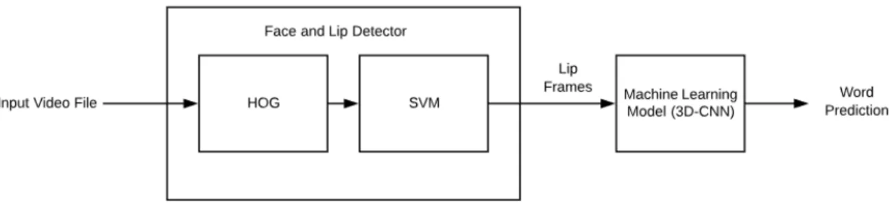
In order to train a model to recognize spoken words, accurately detecting lips in the frames of a video is essential. We will develop a pipeline for assembling 3D data packages of lip frames from short videos taken from a dataset of words from television programs. High-level face detection algorithms will first be used to assist in building the lip detector framework. The facial detection algorithms used are based upon the principles of Histogram of Oriented Gradients (HOG) and Support Vector Machines (SVMs), which are commonly used algorithms in the field of computer vision. A top-level flowchart of this process can be seen in Figure 1.2

1.3 Scope of Thesis

(16)

Figure 1.2: Top Level Flowchart

accuracy close to that achieved in recent VSR research, at least 60%. Lip detection algorithms and framework must be applied to the thousands of videos in the dataset in order to prepare the data needed during the machine learning phase. The machine learning phase will then attempt to train the 3D-CNN using the lip data to identify spoken words.

(17)

Chapter 2

BACKGROUND

2.1 Overview

This chapter outlines the relevant theory and literature used throughout this thesis. The theoretical areas of the thesis are broken down into two larger parts: computer vi-sion and machine learning. Computer vivi-sion is used to address the face detection and lip detection. The face detection algorithm employs Histogram of Oriented Gradients (HOG) for feature selection and Support Vector Machine (SVM) for classification. Machine learning consists of the implementation of the 3D convolutional neural net-work and its training and subsequent testing. Lastly, the most relevant literature on Visual Speech Recognition will be reviewed.

2.2 Face and Lip Detection

Facial detection has seen great advancements in the past decade and its use can be seen in everyday technology, such as auto-focus on smartphone cameras. Software is used to detect the faces in a digital image and then the camera is focused on those detected faces. Any facial identification system uses a face detection algorithm for its first stage; you need to detect a face before you can begin to identify it!

(18)

face and putting a bounding box around each detected face as verification as seen in Figure 2.1.

Figure 2.1: Example Output of a Face Detection Program [17]

Algorithms used for face detection include Classifier-Cascades (Viola-Jones), Eigen-faces, Cross-correlation, Neural Networks, Principal Component Analysis, and many more [44] [15]. This paper will use an algorithm based on Histogram of Oriented Gradients and Support Vector Machine and will provide a background and review on each [39].

2.2.1 Digital Image Representation

(19)

associated with it that describes its color. The left grid shows what the image would look like and the right grid shows the corresponding 2D array of pixel values.

Figure 2.2: Digital Image Representation [10]

For this example, the pixel values are normalized between 0 and 1 but in a standard 8-bit image the values would be between 0 and 255. A pixel value of 0 corresponds to completely black and a pixel value of 255 (or 1 in the normalized case) corresponds to completely white. Since this is a gray scale image the array is 2D which corresponds to the height and width of the image (in pixels). The image of the letter ’a’ in the example is a 14x12 array.

(20)

Figure 2.3: Representation of Digital Color Images as 3D Array [13]

Every subsequent concept in computer vision builds on this idea of treating images as arrays of pixel values. Doing this allows images to be broken down into a set of numeric data which can then be used in computations with various algorithms.

2.2.2 Histogram of Oriented Gradients

Histogram of Oriented Gradients, known in the computer vision world as HOG, is a commonly used feature representation for object detection. Its use for human detection was first presented in [39] in 2005. HOG has shown great success in person detection and has been further applied to the problem of face detection. Although HOG has seen an increase in use for face detection it is worth mentioning that the Viola-Jones object detection framework, which makes use of Haar features, is still the predominantly used algorithm for face detection. The HOG technique is chosen for this paper for two reasons: it has easier to use open-source implementations and is more easily adapted to perform lip detection instead of face detection.

(21)

involves comparing the adjacent pixel values and finding the direction that the image is becoming lighter, or increasing in pixel value. To demonstrate this, consider the example shown in Figure 2.4 where the gradient vector will be calculated for the pixel highlighted in red.

Figure 2.4: Calculating the Gradient Vector [19]

The pixel values are increasing upwards with a magnitude of 93 −55 = 38, and towards the right with a magnitude of 94−56 = 38. Combining these two changes as vectors in thex and y directions gives a resultant gradient vector shown in Figure 2.5. This process is repeated for every pixel location in the image, except for edge pixels.

(22)

Figure 2.5: Resultant Gradient Vector [19]

the sum of the magnitudes of each gradient vector in that direction. A bin size of 20 degrees is typically chosen (as seen in Figure 2.7).

Each cell is then represented by the vector orientation that is most frequent in the histogram. This process is then repeated for every cell in the image until each cell has a gradient vector to represent the pixel change in that localized area of the image. This process significantly reduces the dimensionality and size of the image data when compared to using the raw pixel values. When performed on an image of a human face the output is shown in Figure 2.8. The HOG representation basically shows the flow of light across the image from dark to light (increasing pixel values).

(23)

Figure 2.6: 8x8 Cell for HOG [20]

from images with faces in it and will then decide if the HOG feature vector is a positive or negative match to the class of images it has been trained on.

2.2.3 Support Vector Machine

Support Vector Machine, commonly referred to as SVM, is a widely used classification algorithm in the world of machine learning. It is a supervised learning model that performs binary classification, which classifies an input as belonging to one of two possible classes. The key feature of the SVM is that it finds the optimal hyperplane between two classes by utilizing an allowable margin for overlap between the two classes [53] [9].

(24)

Figure 2.7: Histogram Used in HOG [20]

it lies on. Drawing a line to separate the two classes is easy enough and the green line on the figure is just one of many options, but how can SVM decide which line is the optimal line? The key concept of SVM is that the classifier boundary should be as far away from each class of data point as possible; notice how the green line is about equal distance from the black data points and the blue data points. This is achieved by carefully considering the margin when calculating the classifier.

(25)

Figure 2.8: Input Image (left) and Output of HOG (right) [16]

Figure 2.9: SVM Example for 2D Dataset [9]

The next step in the SVM process is to determine the equation for the margin lines. Since the goal of SVM is to find the line (w and b values) that best separates the classes, the classifier equation is applied to the points closest to the boundary. For the blue points closest to the point the equationwT_x₊_b _{= 1 is used and for the red}

points the equation wT_x₊_b ₌ ₋_{1 is used [57]. This is done to generate a margin}

that can be used to best separate the two different classes.

(26)

Figure 2.10: SVM Example with Boundary Equations [57]

wT

kwk(x+−x−) =

wT_(x

+−x−)

kwk =

2

kwk

The next step in the derivation is to find the boundary equation by maximizing the margin between classes. This is considered a constrained optimization problem and is formulated using the Lagrange multiplier [53].

The primal formulation is then, where yi are the individual training sample labels

(yi{−1,1}) and α is the vector of Lagrange Multipliers:

minL(w, b, α) = 1 2kwk

2 −

n

X

i=1

αi[yi(wTxi+b)−1]

Maximizing the margin is the same as minimizing the magnitude of the weight vector. Using this and rewriting the primal formulation with the weights in terms of the training data, and substituting in leads to the dual formulation:

maxL(α) =

n

X

αi−

1 2

n

X

(27)

subject to: Pn

i=1αiyi = 0, αi ≥0

These equations are then solved using quadratic programming and the discriminant function is found to be:

g(x) =X

i

αiyi(xTi x) +b

Sometimes attempting to find a boundary with zero misclassifications is not possible due to noise and outliers in the data to be classified, this issue is solved by the introduction of asoft margin. This introduces a new parameterC which changes the optimization problem to:

min1

2kwk

2 +C n X i=1 ξi

subject to yi(wTxi+b)≥1−ξi

In this situation C acts as a regularization parameter that controls the effect of the constraints andξis a ’slack’ variable that is used to determine when a sample is either a margin violation or a misclassification. A small C value will allow constraints to be easily ignored which results in a large margin, where as a large C makes constraints much harder to ignore which results in a small margin. A hard margin where all constraints must be followed is the case where C is equal to infinity, which is simply the base case first presented [57].

(28)

SVM used in the face detection algorithm operates in a much higher dimension space and as such utilizes a boundary hyperplane.

For the specific problem of face detection, a sliding window search strategy was em-ployed where classification is performed on different windows in the image. SVM compares the feature vector generated by HOG to other feature vectors of known classes. First, HOG is applied to training images of faces and images of non-faces. Each image is then associated with an output feature vector. These output feature vectors are then used to train the SVM for classification. The trained SVM will then perform the classification on HOG feature vectors.

If the sliding window search method identifies multiple potential bounding boxes, as it commonly does, only the best fit box will be returned. Choosing of the best fit box is done via non-maximum suppression (NMS). NMS starts with the bounding box that has the highest score, which in the case of the SVM would be the distance from the boundary equation, and suppresses all other boxes that overlap it [50].

2.2.4 Lip Detection

Following the face detection lip detection is performed by detecting the key facial landmarks using a shape predictor. The shape predictor to be used is based off of [46] and makes use of an ensemble of regression trees. This method is chosen because its speed allows for real time detection. An example of the output of a shape predictor used in conjunction with a face detector is shown in Figure 2.11.

(29)

Figure 2.11: Example Output of Facial Landmark Detection [18]

out of the image. The mathematical background presented in [46] is intense and is not the focus of this paper so is left out.

2.2.5 Data Processing

The last step before going on to the model training is the preparation of the data extracted using the lip detector. Since the goal is to form a 3D array by adding a time dimension to the already existing spatial dimensions, each frame is converted to grayscale from color. If the images were not converted to grayscale each frame would already be 3D and the time dimension would then make the output array 4D in nature. Minimal research has been done on 4-Dimensional CNNs and few implementations exist.

(30)

resized to a common size in order for them to be compatible for stacking. After each frame is resized they are all stacked together to form a 3D array. Each frame of lip data is 2D and there are multiple frames in each video which adds a third dimension, time, to the data. Figure 2.12 shows a visualization of the stacking of 2D arrays.

Figure 2.12: Stacking 2D Arrays to form a 3D Array [25]

2.3 Convolutional Neural Networks

(31)

2.3.1 Neural Networks

Although there is a large difference between traditional neural networks and CNNs due to their layer composition, there are a lot of similarities in the construction and training of each. Before we can fully understand the principles behind CNNs it is important to first understand NNs and their basics.

The most common use for NNs is to take a set of input data and then classify it into different groups. They work by having layers of neurons, modeled off the neurons in a human brain, that connect to each other and help the network make decisions and learn patterns in data [7]. An overview of a simple neural network structure can be seen in Figure 2.13.

Figure 2.13: Architecture of a Simple Neural Network [28]

(32)

in red), an output layer (shown in green), and a variable amount of hidden layers (shown in blue).

Input layers are simply just the direct input values of the data being fed to the network. The output layer is the layer tasked with performing classification of the input data and the size usually corresponds to the number of classes in the dataset. If the task of the NN is to predict a number based on a picture of a handwritten digit, the ’classes’ would be the numbers 0, 1, 2, 3, 4, 5, 6, 7, 8, and 9. Since there are ten different classes the NN would have 10 output neurons. The output neuron with the highest value after the input is fed into the network would be the predicted class. The hidden layers are what gives the NN more complexity and allows it to perform more difficult tasks. More hidden neurons equals more parameters which allows the network to learn more complex patterns in the data.

Another important note about NNs is that each neuron is connected to every neuron in the previous layer and every neuron in the next layer. Consider the example shown in Figure 2.14 which shows 5 input neurons connected to two hidden neurons.

(33)

The values in the input neurons are denoted by x1, ..., x5, while the values in the

hidden neurons are denoted by z1 and z2. Let the weights be denoted by wij for the

connection between input i, and neuron j in the next layer. The value z1 can then

be expressed as a summation of the inputs and weights according to:

z1 =w11x1+w21x2+w31x3+w41x4+w51x5

The value of the weights is determined during training which will be covered in a later section. The z1 value is then put into an activation function and the output of that function is the value held in the neuron. Activation function are used to increase the non-linearity of the network and help it realize more complex functions and patterns. Some commonly used activation functions for neural networks include the sigmoid function and the rectified linear unit (ReLU). These functions are included below [27].

Sigmoid: σ(z) = _1+e1−z =

ez

ez₊₁

ReLU: R(z) =z+ ₌_max₍₀_{, z}₎

Graphs of these two activation functions are included in Figure 2.15 to demonstrate the non-linear nature of each function.

(34)

2.3.2 Model Architecture

Now that the basics of neural nets have been covered, it is now appropriate to review the theory on CNNs, as they are the machine learning model that will be implemented in this paper. First, we will cover the architecture of CNNs and how they relate to NNs.

Firstly, consider the CNN architecture shown in Figure 2.16, this network is used to classify images into categories such as car, truck, van, bicycle, etc. The network consists of multiple different types of layers that each behave differently. There are three main types of layers: Convolutional, Pooling, and Fully Connected. This differs from a NN where each layer operates the same but has a variable amount of neurons [11].

Figure 2.16: Architecture of a Common CNN [11]

(35)

filter is a 2D array of numbers (the values of which are determined during training just like weights in a traditional neural network), also called a convolutional kernel, and in this case the filter size is 3x3 (which is the most commonly used size, with 5x5 the next most common).

The filter values and the image values in the neighborhood around the center pixel are multiplied via 2-dimensional dot product and added to replace the center pixel (the purple square in the right array). This is performed by multiplying the values from each matching location in the filter and image and then summing all the products together for the neighborhood. This process is repeated for every area on the image that the filter can fit on and the output values are stored in a new array that is the result of the convolution. All of these values are then input into an activation function, which for CNNs is most commonly the ReLU activation function, and the result is the output of the convolutional layer [12].

Figure 2.17: Example of a Filter Being Convolved Around an Image [12]

(36)

traditional max pooling layers take a 2x2 area and replace it with the max value of the area. This reduces the size of the data by half in each direction. A visual example is included in Figure 2.18 that demonstrates both max and average pooling.

Figure 2.18: Max and Average Pooling Example [11]

The combination of input, convolution, ReLU activation, and pooling layers is what makes up thefeature learning section of the CNN; this section performs unsupervised feature extraction. The second section of the CNN performs classification. This classification section of the CNN is actually just a standard neural net as described previously. This can be seen in the right section of 2.16.

Since the output from the feature learning section of the CNN is 2D but a standard neural net only accepts 1D inputs, the 2D output must be flattened, as seen in the first layer of the classification section in Figure 2.16. The flatten layer converts the 2D data array to a 1D data array. After the data has been flattened it is then input to the classification NN as described in the previous section. In CNNs these standard NN layers are called fully connected layers since each neuron is connected to every neuron in the layers before and after it.

(37)

value then the CNN chooses class 2 as the most probable selected class for the input image [12]. Softmax is chosen instead of a traditional max because it also rescales output values to be between 0 and 1, where all the output values summed together equal 1. Doing this allows the values to also be interpreted as a prediction confidence rating. If the model predicts class 2 with a value of 0.65 it is much more certain of the prediction than if it predicts class 2 with a value of 0.21.

2.3.3 Model Training

Model training enables a neural network to recognize patterns and make decisions or classifications from data. It is essential in machine learning. Before we can talk about the mathematics behind CNN model training we must first discuss what the model will be trained with. Data used for training a model is called the training dataset and data used for testing a model (after it has been trained) is called the test dataset. It is important that samples used in the training dataset are not also present in the test dataset. Showing the model samples from the test set invalidates results because it is important to grade neural networks on their ability to classify unseen data.

(38)

Training datasets are generally much larger than test datasets. In addition to training and testing datasets there are validation sets. Validation sets are used to check the performance of the model after each training cycle, allowing ML engineers to tune hyper parameters on the fly, such as filter size, stride, or filter count, but is not used for model learning. The test set is used after training has been completed to grade the performance of the network. Although it is not uncommon for validation and test sets to be used interchangeably since neither set is shown to the model during training. A traditional approach is to use 70% of the data for training and 30% for testing and validation but this is just a suggestion and other splits have worked well too [4]. This split is visualized in Figure 2.19.

Figure 2.19: Split of Data into Training, Validation, and Test Datasets [4]

Model training consists of two important steps. First an input is fed into the model and moves forward through each layer to the end of the network. Then the expected output is compared to the actual output and the loss is calculated. This loss is then propagated backwards through the network to update the weights in a process known as back-propagation.

(39)

0 0 1 0 0 0 0 0 0 0 T

As can be seen there is a 1 in the 3rd location in the label vector, which is the class that the training sample belongs to, and a 0 in all the other locations since the sample is not a member of those classes. Next, the sample data is input into the network and moves forward through the network. For example say that the sample output is a vector of:

0.22 0.11 0.76 0.30 0.09 0.16 0.19 0.23 0.13 0.32 T

This sample would be correctly classified because the value in the third location is the highest value so the model would choose class 3 as its predicted class. Although the model predicted the sample class correctly there is a still an error vector associated with the training sample. The error vector is calculated based on the desired loss function being used (of which there are many). For a multi-class classification problem (where the number of classes ¿ 2) a standard loss function used is categorical cross-entropy, which is what is used in this paper. Cross entropy is also called log loss, and uses the following formula whereyd is the desired output and ya is the actual output

[21]:

loss(yd, ya) =−log|1−yd−ya|

(40)

when the actual value is close to 1 the loss is small, and when the error is far from 1 it is much larger.

Figure 2.20: Cross Entropy Loss Function when Desired Output is 1 [21]

After the loss is calculated at each neuron in the final layer of the network, this value is then propagated backwards through the network, correcting the weights between each neuron. The goal of this is to correct the weights that are most responsible for the loss. The principle of back propagation is based on gradient descent [42].

As defined in the previous section, the neuron value before the activation function (otherwise known as the induced local fieldv(n), where n is the iteration through the training data) for neuron j is:

vj(n) = X

i

wij(n)yi(n)

Where yi(n) is the output of the neurons in the previous layer and wij(n) is the

(41)

yj(n), of the neuron after applying the activation function for neuron j, ϕj(n), is

then:

yj(n) =ϕj(vj(n))

Each neuron has an instantaneous error energy associated with it defined using the least-mean squared algorithm, whereej is the error function being used:

εj(n) =

1 2e

2 j(n)

Next step is to find the partial derivative of the error energy with respect to the weight vector. This is done using the chain rule of calculus:

∂εj(n) ∂wij(n) =

∂εj(n) ∂ej(n)

∂ej(n) ∂yj(n)

∂yj(n) ∂vj(n)

∂vj(n) ∂wij(n)

One thing to note is that the ReLU activation function is not differentiable at 0. This is solved by setting the derivative equal to 0 at that point. Next, differentiating both sides of the instantaneous error energy equation leads to:

∂εj(n)

∂ej(n) =ej(n)

Using a simplified loss function ofej(n) =yd(n)−yj(n), the partial derivative is then:

∂ej(n) ∂yj(n)

(42)

Then differentiating the previously defined equation ofyj(n) =ϕj(vj(n)) gives:

∂yj(n) ∂vj(n)

=ϕ0(vj(n))

Lastly, differentiating the previously defined equation ofvj(n) = P

iwij(n)yi(n) gives:

∂vj(n) ∂wij(n)

=yi(n)

Now substituting these individual partial derivatives into the chain rule equation leads to:

∂εj(n)

∂wij(n) =−ej(n)ϕj

0

(vj(n))yi(n)

The delta rule is then used to define the weight correction as:

∆wij(n) = −η

∂εj(n) ∂wij(n)

In this equation η is the learning rate parameter which is one of the most important parameters in model training. Combining the two previous equations yields:

∆wij(n) = −ηδj(n)yi(n)

(43)

δj(n) =

∂εj(n) ∂vj(n)

=ej(n)ϕj0(vj(n))

As can be seen in the previous equation the local gradient for the neuron is equal to the product of the error signal for that neuron and the derivative of the activation function. From this equation the weight adjustment for each connection can be calcu-lated. Analyzing the equation it can be seen that the error signal is a key component to the weight update. The error signal can be broken into distinct cases: when the neuron is an output node and when it is a hidden node [42].

The output node is a more straightforward case since the desired output is provided by the label associated with the training sample. The loss function is simply the previously defined function of ej(n) = yd(n)−yj(n).

The more complicated case is when the neuron is a hidden node since there is no explicit desired response value such as the training label for output nodes. This means that the error signal must be propagated backwards from the output nodes to the hidden nodes. The first step in this is redefining the formula for the local gradient:

δj(n) =−

∂εj(n) ∂yj(n)

∂yj(n) ∂vj(n) =−

∂εj(n) ∂yj(n)ϕj

0

(vj(n))

Next the partial derivative of the error energy must be calculated using the formula:

εj(n) =

1 2

X

k

e2_k(n)

(44)

∂εj(n) ∂yj(n)

=Xek

∂ek(n) ∂yj(n)

Combining this with previously defined equations leads to:

∂ek(n) ∂vk(n)

=−ϕk0(vk(n))

Differentiating the previously defined formula for the induced local field, vk(n) =

P

iwk i(n)yi(n), gives:

∂vk(n)

∂yj(n)

=wk j(n)

Combing the previous two equations gives:

∂εj(n) ∂yj(n)

=−Xδk(n)wk j(n)

Now finally substituting this equation into the error signal equation gives the local gradient for hidden neurons:

δj(n) =ϕj0(vj(n))

X

δk(n)wk j(n)

Now that the local gradient has been defined we can revisit the formula for weight correction:

(45)

∆wij(n) is the weight correction from neuroni to neuron j. δj(n) is the local gradient

as previously defined in the proof. yi(n) is the input signal from neuron i that feeds

into neuron j. η is the learning rate parameter that is controlled during the model training. This parameter has a major impact on the model during training, if it is too small training could take much longer than necessary as weights update too slowly, wasting valuable time. If the learning rate is too large then large values of loss can propagate backwards too strongly through the network and ruin previously defined network weights [42].

The weights are then recalculated based on a concept called batches. A batch size of 1 means that the weights are recalculated after every individual training sample. More commonly a batch size of 16 or 32 is used in training [45]. This means that the weight correction, ∆wij, is added together for 16 or 32 samples and then updated

each time the batch size is reached.

Each time the full set of training samples is used for weight correction is called an epoch. In general, the more training epochs you can run the better but real life time constraints exist. It is generally chosen to use as many epochs as time and hardware allows for which could be 10, 100, 1000, or more based on the set of training data being used.

After each training epoch the data should be randomized in order to help reduce overfitting. As stated before increases in variance in the data presented during train-ing helps reduce overfitttrain-ing. Reshuffltrain-ing the data helps the model avoid focustrain-ing on specific patterns in the training data and focus on general patterns instead.

(46)

2.3.4 Model Testing

After training the model is tested using the test dataset previously set aside. This dataset is what is used to grade the performance of the model.

When testing the model each sample is pushed forward through the network but no back propagation happens because the model is done learning. After being pushed forward through the network, the model makes a prediction on the class of the input based on the max neuron value in the output layer. This prediction is compared to the known label, since the test dataset is labeled in the same manner as the training and validation sets.

After testing each sample in the test dataset the number of misclassifications is used to calculate the accuracy using the standard formula:

Accuracy= T otalSamples−M isclassif ications

T otalSamples ×100

2.4 Related Works

The problem of VSR has been explored in [36], [35], [54], [43], and [38], among other works.

(47)

Figure 2.21: Architectures Used in Lip Reading in the Wild Paper [36]

words taken from TV programs. This differs greatly from most VSR datasets that are recorded and assembled in a controlled lab environment, and is a better approximation of the videos seen in real-life classification tasks.

The second proposal of [36] is to investigate the performance of different CNN ar-chitectures for recognition of the previously assembled dataset. They test the per-formance of 4 different architectures, two 2D-CNNs and two 3D-CNNs, and achieve a top recognition rate of 61.1% using a 2D CNN architecture with multiple input towers that are concatenated after performing one convolution on each frame. The architectures used in [36] are shown in Figure 2.21.

(48)

width of each frame, H is the height of each frame, 25 is the number of total frames per video (the temporal dimension), and 3 is the multi-channels of the color image. Our paper uses the conventional notation that CNNs with 3D inputs are considered ’3D CNNs’ especially since they perform 3D-Convolutions at the layer level.

The architecture used in this work is most similar to the EF architecture. The main differences between our architecture and the EF architecture is the number of pooling layers, number and size of fully connected layers, and the number of frames that make up the input to the network. We use significantly less than 25 frames due to the observation that the duration of most words is less than 25 frames, and by including too many frames recognition rate could actually be worsened by the inclusion of information unrelated to the target word.

Lip Reading Sentences in the Wild [35], authored by the same team as [36], takes the work done in [36] and extends it a step further. Where [36] focuses on assembling a dataset of spoken words from TV programs, [35] focuses on assembling a dataset of spoken sentences from TV programs. [35] uses essentially the same pipeline as [36] with minor modifications to assemble the new dataset. The task of recognizing the spoken words is made much more difficult by the fact that the data is now sentences of variable length rather than videos of fixed length containing one word. This requires a more sophisticated ML model(s) than the one used in [36] and also requires the use of audio data during training which was not used in [36].

(49)

a linear cosine transform (known commonly as Mel Frequency Cepstrum, MFCC) followed by LSTM modules. The second section of the model uses the outputs from the audio and visual halves as an input into a second group of LSTM modules and attempts to assemble words and match visual and audio data [35].

This structure of two or more separate ML models is commonly used in VSR tasks that require full decoding of sentences. This model structure can be seen in Figure 2.22. The second half of this problem, assembling words from phonemes or visemes, is similar to that in standard ASR and is explored in [51] and [49]. Both these papers show the success of using Hidden Markov Models (HMMs) for speech recognition.

Figure 2.22: Overview of Traditional AV-ASR Programs

(50)

from the same video) closer together and push impostor pairs (audio and visual data from different videos) farther apart.

(51)

Chapter 3

METHODS & IMPLEMENTATION

3.1 Overview

This section will lay out the actual software and mathematics used to implement the model used for visual speech recognition. A block diagram of the overall work is shown in Figure 3.1.

Figure 3.1: Overview of Thesis Work

3.2 Dataset

Before any code can be written, the first actual step in the project is to decide and compile the dataset to be used. Compiling a comprehensive VSR dataset is a complicated task due to the difficulty of finding and labeling data. In this situation the data is a video of a speaker and the label is the spoken word or group of words. This task has been discussed in [36] and [35].

(52)

this dataset to various other datasets used in VSR research, and is pulled directly from [36].

Table 3.1: Comparision of Various Datasets [36] Name Env. Output I/C # class # subj. Best perf.

AVICAR In-car Digits C 10 100 37.9%

AVLetter Lab Alphabet I 26 10 43.5%

CUAVE Lab Digits I 10 36 83.0%

GRID Lab Words C 8.5 34 79.6%

OuluVS1 Lab Phrases I 10 20 89.7%

OuluVS2 Lab Phrases I 10 52 73.5%

OuluVS2 Lab Digits C 10 52

-LRW TV Words C 500 1000+

-The major differences between LRW and other datasets is the environment, number of classes, and number of subjects. Each video in the LRW dataset is cut out of a TV program on BBC, which is what gives it its In the Wild moniker since videos are not recorded in a controlled lab environment (AVICAR is the only other dataset not recorded in a lab). I/C stands for isolated and continuous, samples in the LRW dataset are single words cut out of an entire sentence, further adding to the more natural and in the wild nature of the data. LRW also has 500 different spoken words making it the largest of the available datasets and has over 1000 different speakers which is significantly more than any other dataset. For a combination of these reasons, the LRW dataset has been one of the most popular datasets for speech recognition research tasks.

(53)

to 9/30/2016 and also contains 50 samples per class [36]. From the date range it is clear that there is no overlap between subsets since all videos are pulled from new broadcasts. These statistics are shown in Table 3.2.

Table 3.2: LRW Dataset Statistics [36]

Set Dates # class # per class

Train 1/1/2010-8/31/2015 500 800-1000 Validation 9/1/2015-12/24/2015 500 50

Test 1/1/2016-9/30/2016 500 50

Each sample is a video containing 29 frames, at a frame rate of 25 frames per second, for a total duration of 1.16 seconds each. For each sample the word occurs in the middle of the video. Included with each video is metadata that gives the duration of the word, which could be used to determine the exact starting and end frames. All videos are included as mp4 files and are labeled using the format ’WORD.mp4’, such as ACCORDING.mp4 for a sample thats class is the word ’according’ [36].

3.3 Classification and Accuracy Goals

(54)

Table 3.3: 100 Word Subset of the LRW Dataset

ABOUT ABSOLUTELY ABUSE ACCESS ACCORDING

ACCUSED ACROSS ACTION ACTUALLY AFFAIRS

AFFECTED AFRICA AFTER AFTERNOON AGAIN

AGAINST AGREE AGREEMENT AHEAD ALLEGATIONS

ALLOW ALLOWED ALMOST ALREADY ALWAYS

AMERICA AMERICAN AMONG AMOUNT ANNOUNCED

ANOTHER ANSWER ANYTHING AREAS AROUND

ARRESTED ASKED ASKING ATTACK ATTACKS

AUTHORITIES BANKS BECAUSE BECOME BEFORE

BEHIND BEING BELIEVE BENEFIT BENEFITS

BETTER BETWEEN BIGGEST BILLION BLACK

BORDER BRING BRITAIN BRITISH BROUGHT

BUDGET BUILD BUILDING BUSINESS BUSINESSES

CALLED CAMERON CAMPAIGN CANCER CANNOT

CAPITAL CASES CENTRAL CERTAINLY CHALLENGE

CHANCE CHANGE CHANGES CHARGE CHARGES

CHIEF CHILD CHILDREN CHINA CLAIMS

CLEAR CLOSE CLOUD COMES COMING

COMMUNITY COMPANIES COMPANY CONCERNS CONFERENCE

CONFLICT CONSERVATIVE CONTINUE CONTROL COULD

The full training set (800-1000 samples per class) for the first 100 words will be used. It was chosen to use all the samples of a subset rather than use all classes but with fewer samples. Using fewer samples per class has been shown to have a strong negative affect on neural net accuracy [36].

The validation accuracies presented in [36] will serve as the benchmark as it has the current state-of-the-art results on the LRW dataset using a CNN. The results from the four CNN architectures tested in [36] are 44% and 46% for the two 3D architectures and 57% and 61% for the two 2D architectures. These results are for classifying the entire 500 word dataset.

(55)

accuracy of the models in classifying the 333 word subset all see substantial increases and the new highest accuracy is 65%.

Rather than remove plurals and viseme ambiguities this thesis includes them since the dataset is already being restricted to a 100 word subset. This keep the problem both complex and challenging when compared to other VSR works. It is expected that word combinations such as BENEFIT-BENEFITS, CHANGE-CHANGES, and CHARGE-CHARGES, all of which are present in the 100 word subset, will make successful classifications more difficult. Due to this slightly different dataset used in comparison with [36] it is difficult to draw exact comparisons but the goal is to achieve similar performance classifying the 100 word dataset with pluralities to the results of the 333 word dataset.

3.4 Hardware

All processing and model training was performed on a Nvidia GeForce 2080 Ti GPU with an Intel Zion 2.1Ghz processor, 16-core CPU, with 32GB of RAM. The machine had Ubuntu 18.04.3 64-bit operating system with kernel version 4.15.0-65 and CUDA version 10.0.13.

3.5 Software

(56)

NumPy is a scientific computation library that is excellent for array based operations. Much of machine learning is based in linear algebra concerning vectors and arrays, which makes NumPy hugely popular and important. In addition to this library,SciPy can be used for further advanced computation and Scikit for implementing specific ML algorithms and data mining [31].

In addition to these libraries are Keras and Tensorflow. Tensorflow is one of the premier open source library for handling complex back-end ML operations [32]. It is written in C++ and Python, and also developed and maintained by Google Brain, giving it great reliability and flexibility. Keras is another open sourced library specif-ically for neural networks and written in Python [34]. Keras is primarily used in conjunction with Tensorflow, as a front-end API that is extremely easy to use with Tensorflow as the powerful back-end. This combination of Keras and Tensorflow makes Python one of the most popular languages used when dealing specifically with neural networks [31].

In addition to the neural network implementation is the lip detector module. The lip detector module is based off the dlib face detector. Dlib is an open source computer vision and machine learning library written in C++ with easy to implement Python APIs. Dlib is one of the most widely used face detection softwares for two reasons: it is fully open source and is available for both commercial and academic use, and it is also one of the fastest implementations available since it is written completely in C++ [14].

(57)

10 years ago and is the largest open source computer vision project in existence and has extensive support for many applications [3].

Other specific, but minor, software packages used during implementation will be men-tion as they are used. The main software packages used are the previously menmen-tioned Numpy, Dlib, OpenCV, and Keras with Tensorflow.

3.6 Lip Detection

This section will discuss the actual implementation from a software standpoint for building the lip detection framework. This includes the lip detector module to be applied to each video, the framework for applying it to every sample and storing the result, and the framework for making the accompanying labels for each sample.

3.6.1 Lip Detector Module

The lip detector module is built primarily off the dlib face detection package as described previously. It will also make use of theOpenCV library for handling video files, Numpy for converting videos and images to usable arrays and storage of those arrays, and also imutils, an open source library developed by Adrian Rosebrock of Pyimagesearch, which is a series of OpenCV convenience functions [22].

The first step our module performs is to load dlib’s predefind face detector. The face detector then requires a path to the Dlib shape predictor file. The shape predictor is a ’.dat’ file provided directly from dlib and is included in the same directory as the source code. This is performed using the following code:

(58)

detector = dlib.get_frontal_face_detector() # Initialize detector

predictor = dlib.shape_predictor(predictor_path) # Load predictor

For this project we are using the 68 point facial landmark detector as can be seen in the first line of the code above. Dlib’s face detector makes use of the HOG and SVM algorithms outlined previously in the background chapter. The 68 point detector can be seen in Figure 3.2.

Figure 3.2: 68 Point Facial Landmark Detector Used by Dlib [18]

This detector is chosen over smaller, faster detectors, such as the 5 point predictor, due to the later need of isolating just the lip region. This is easily done by referring to a subset of the predictor points.

(59)

while(video.isOpened()):

ret, frame = video.read() # Capture frame

In addition to the actual video frame, the video.read() function returns a boolean value that is used to check if the frame exists. If the frame exists, it is then time to process the frame and apply the face detector. An example of all the frames in a sample video is included in Figure 3.3

Figure 3.3: Frames in a Sample Video

(60)

more computing with minimal increases in performance [33]. Each frame will also be resized to a standard size before being placed in the lip detector. The frame will then be input into the previously initialized lip detector. The code for this is as follows:

frame = cv2.cvtColor(frame, cv2.COLOR_BGR2GRAY) # Convert to grayscale

frame = cv2.resize(frame,(224,224)) # Resize image

faces = detector(frame,1) # Detect faces in image

The frames are all resized to be 224 pixels by 224 pixels in order to reduce processing time for frames of greater size (and since this size is known to work with this face detection implementation). The 1 argument to the detector function means to up-sample the image 1 time, which helps the detector find smaller harder to detect faces. Since we know each sample has exactly one speaker, if the detector detects more than 1 face or 0 faces then that video sample is discarded. This is acceptable due to the abundance of training data for every class.

The face object that is returned from the detector is then input into the shape pre-dictor to identify the locations of the landmark. The output of the shape prepre-dictor is converted to a Numpy array for convenience, using the imutils library. This is shown in the following code.

shape = predictor(frame,face) # Identify facial landmarks

shape = face_utils.shape_to_np(shape) # Convert shape to numpy array

(61)

A margin of 10 pixels is included to grab excess information around the lips as just using the strict landmarks tends to be too tight of a crop and some information is lost. This is always possible since each video includes a much larger area than just the face, as shown in Figure 3.3. This bounding rectangle is then applied to the frame to grab the required lip data. Lastly, the lip data is resized to a common size for concatenation compatibility. The code for this is included below.

(x, y, w, h) = cv2.boundingRect(np.array([shape[48:68]])) # Find bounding box

margin = 10 # Extra pixels to include around lips

lips = frame[y-margin:y + h + margin, x-margin:x + w + margin] # Grab lips

lips = cv2.resize(lips,(100,60)) # Resize to standard size

The lip frames are resized to 60 by 100 pixels because this will match the first layer of the CNN that it will be input in to. A collection of lips from each frame is shown in Figure 3.4.

Figure 3.4: Detected Lips in Each Video Frame

(62)

arrays to form a 3D array. Afterwards, the array is reshaped using Numpy’smoveaxis function. The array needs to be reshaped in order to be compatible with the first layer of the CNN. The lip detector module accepts a path to a video file as the argument and returns the 3D array of lip frames as a numpy array. A software diagram for the lip detector module is included in Appendix D.

3.6.2 Processing Framework

The tree structure of the dataset is shown in Figure 3.5. Only the first two classes are shown, which are ’About’ and ’Absolutely’, the actual directory structure extends for all 500 classes. Inside each class are 3 folders: test, train, and val, and each folder contains the actual ’mp4’ sample files and a corresponding ’txt’ file that contains the metadata.

(63)

The first function in the processing framework goes through each subfolder in the directory and applies the lip detector module to each mp4 file. If no face is detected in the ’mp4’ file, the program simply skips the file, otherwise the output of the module is the previously mentioned numpy array.

This numpy array is then sliced using standard array slicing methods in Python. The array is sliced to grab the middle 11 frames of the video. This is done to isolate the actual frames that correspond to the word being spoken. Since only part of the video is the target word, it makes sense to discard the extraneous information that does not pertain to the target word. For this reason 11 frames are chosen because it is the closest to the average frame length per word as seen in Table 3.4.

Table 3.4: Duration of Words in LRW Dataset Duration (s) # of Frames

Max 0.8 20

Min 0.09 2.25

Average 0.424 10.6

The resulting numpy array is then stored using the commandnp.save(location,numpy_array). The location for the stored array is the current directory that the input ’mp4’ file is

located. This is chosen for simplicity.

(64)

3.7 Model Training

3.7.1 Label Maker

The first step of preparing the data to be used for training is making the associated labels to accompany the data. Since there are 100 classes in the dataset all the labels will be vectors of length 100. The labels are made corresponding to the class directories located in the ’lipread mp4’ directory. Each label is a vector of all 0’s with a 1 in the location that corresponds to the class. For example, the word ’About’, which is the first class in the dataset will have a label vector of:

1 0 0 0 0 0 0 0 ...

T

Furthermore the label vector for ’Absolutely’, the second class in the dataset will have a label vector of:

0 1 0 0 0 0 0 0 ...

T

Each label vector is stored as a ’.npy’ file using the previously mentioned numpy save command. They are all stored in a ’labels’ directory located on the same level as ’lipread mp4’, just below the ’LRW’ directory.

3.7.2 Assemble Dataset

(65)

than the dimension of each training sample. For example if the training dataset is 100 images of size [50,200] then the dimension of the training array will be a 3D array of size [100,50,200].

For our project each input into the CNN will have size [11,60,100,1], the 4th dimen-sion of 1 is needed for CNN compatibility, since convolution operations will expand that dimension it needs to be initialized before training. This leads to an array size of [X,11,60,100,1], whereX is the number of samples in each set. For the 100 class subset the test set contains 4919 samples, the training set contains 95991 samples, and the validation set contains 4937 samples. Each numpy array is built using Python’s built in ’append’ function.

At this point it is important to normalize all the data to be between 0 and 1, this is a step that is usually performed when training neural networks in order to keep loss from destabilizing the model. Every value in the array is divided by 255.0 to convert to the proper range (since pixel values range from 0 to 255).

Dividing by 255.0 converts each value from a unsigned 8-bit integer (uint8) to a float. The standard float type in Python is a 64-bit value (float64). This means that each dataset now takes up 8 times as much memory. Using the standard float type for the 100 class dataset leads to a memory requirement of:

95991×11×60×100 = 6,335,406,000F loats×8Bytes/F loat= 47.2GB

(66)

3.7.3 Model Architecture and Initialization

From this point on, all model intialization, training, testing, etc. is done using the Keras API with Tensorflow-GPU backend. The ’model init’ function takes an input shape as its only parameter. It starts by initializing a model using the Keras Sequen-tial API. SequenSequen-tial models are linear stacks of layers and are the traditional choice when building CNNs.

The base 3D-CNN architecture is based off the architecture described in [54] which the authors use for feature extraction. This base architecture will then be altered multiple times in an attempt to increase accuracy. Each of the individually altered architectures and their results will be presented in the Results chapter.

The base architecture consists of four 3D-convolutional layers, three 3D-max pooling layers, and three fully connected layers. The convolutional layers all use a kernel size of 2, which in 3D is a 2x2x2 cube, a stride size of 1, and ReLu activation. Kernel size is the size of the filter in the convolutional layers, and stride is how many pixels the filter moves in each direction between convolution operations. The number of filters start at 16 and increase by a factor of two in each subsequent layer (32, 64, 128). The max pooling layers use a pool size and strides of (1,2,2) with the 1 being in the temporal dimension.

(67)

The base model architecture is shown in Table 3.5 and the code to initialize the base CNN architecture is shown below that.

Table 3.5: Base Model Architecture

Layer Input Size Output Size Kernel Stride Conv1 11x60x100x1 9x58x98x16 3x3x3 1

Pool1 9x58x98x16 9x28x48x16 1x3x3 1x2x2 Conv2 9x28x48x16 7x26x46x32 3x3x3 1

Pool3 5x10x20x64 5x4x9x64 1x3x3 1x2x2

Conv4 5x4x9x64 3x2x7x128 3x3x3 1

Flatten 3x2x7x128 5376 -

-FC1 5376 1024 -

-FC2 1024 512 -

-FC3 512 100 -

-model = Sequential()

model.add(Convolution3D(input_shape=shape,filters=16,kernel_size=3,strides=1,activation='relu'))

model.add(MaxPooling3D(pool_size=(1,3,3),strides=(1,2,2)))

model.add(Convolution3D(filters=32,kernel_size=3,strides=1,activation='relu'))

model.add(Flatten())

(68)

model.add(Dropout(0.5))

model.add(Dense(512, activation='relu'))

model.add(Dropout(0.5))

model.add(Dense(100, activation='softmax'))

3.7.4 Model Training Script

The model training script begins by calling the previously defined function to build the training and validation dataset and labels arrays. Next it uses the other previously defined function to initialize the Keras CNN model.

Next the model is compiled using the standard Keras ’model.compile’ function. A stochastic gradient descent (SGD) optimizer is used with learning rate equal to 0.02 and Nesterov momentum. SGD is an iterative method that is used to perform the weight updates during model training. Nesterov momentum is used to speed up the training process by accelerating gradient vectors in the right direction [26]. The learn-ing rate of 0.02 was the largest rate that was able to successfully train the models from scratch. Since the model architectures used are not well-known architectures with pretrained models available they must all be trained from scratch. A categor-ical cross entropy loss function was used as is standard for multi-class classification problems.

From here the model is trained using the ’model.fit’ function with shuffle set to True. Shuffling the data randomizes the order of the samples presented to the model each training epoch. This is another parameter used to help reduce overfitting.

(69)

(70)

Chapter 4

TESTING AND RESULTS

4.1 Face and Lip Detection

The face and lip detection program was applied to all video samples for the first 100 classes of the LRW dataset. Once a face was detected, the lips were extracted using the dlib shape predictor landmarks, so all videos that had detected faces had corresponding detected lips. Detecting faces on the other hand did produce some errors. There were two types of face detection errors: no faces detected and more than one face detected (since every video was only one speaker). Samples that had detection errors were discarded from the datasets. Even after discarding the samples with detection errors, there was still enough samples to successfully train the model.

The statistics of the face detection program are shown in Table 4.1. The correct classification rate of 98.62% resulted in enough samples needed to help reach model accuracy goals. The no face error resulted about 3 times as often as the multiple face error but both were relatively infrequent compared to the amount of correct classifications.

The numer of samples of each dataset after processing is shown in 4.2. Each sample was a 4D Numpy array of size (11,60,100,1). The shape of each dataset was then a

Table 4.1: Face Detection Statistics

Type Number Percentage

(71)

5D array with shape (X,11,60,100,1) where X is the number of samples per dataset. The results of the validation set are used to evaluate performance since the dataset was slightly larger than the test dataset. In practice, when the final trained model was tested on both the test and validation datasets the results were negligible. For example, for model #1 the final validation accuracy was 56.98% and test accuracy was 57.32% and for model #6 the final validation accuracy was 63.68% and test accuracy was 63.90%. Furthermore, validation accuracy was recorded after every training epoch so more data was available to draw conclusions.

Table 4.2: Samples per Dataset Dataset Number of Samples

Training 95,991

Testing 4,919

Validation 4,937

4.2 Model Architectures and Results

4.2.1 Model #1

As mentioned in the implementation chapter, multiple different architectures were tested. Each architecture was a modified version of the base architecture presented in the implementation chapter. The base architecture will be considered Model #1 and is shown in Table 3.5.

This model had 6,373,124 parameters (weights) of which 5,506,048 were connections between the last convolution layer and the first fully connected layer. The output of the convolutional section of the network was a vector of dimension 5,376.

(72)

the first model it was used as a test for the training script on multiple machines and training accuracy data from scratch was not recorded.

4.2.2 Model #2

Model #2 was a minor modification on the first model that consisted of adding one more pooling layer and convolutional layer in the hopes that the extra convolutional layer would increase accuracy. After the 4th convolutional layer (the last convolutional layer of the base architecture) another 3D max pooling layer was added, followed by a 5th 3D convolutional layer. In order to accommodate the dimensionality loss from the additional layers, the kernel sizes of both the pooling layers and convolutional layers were changed from 3 to 2. This also allowed us to investigate the effectiveness of kernels of size 2, as most research has been done on CNNs with kernel size 3. The architecture of Model #2 is shown in Table 4.3, with changes from the base architecture bolded.

Table 4.3: Model #2 Architecture

Layer Input Size Output Size Kernel Stride Conv1 11x60x100x1 10x59x99x16 2x2x2 1

Pool3 8x13x23x64 8x6x11x64 1x2x2 1x2x2 Conv4 8x6x11x64 7x5x10x128 2x2x2 1 Pool4 7x5x10x128 7x2x5x128 1x2x2 1x2x2 Conv5 7x2x5x128 6x1x4x256 2x2x2 1

-FC1 6144 1024 -

-FC2 1024 512 -

-FC3 512 100 -

(73)

reduced the total parameters from 46,538,708 to 7,217,364. Despite the reduction in total parameters, Model #2 actually showed an increase in performance. It achieved a peak validation accuracy of 64.84% which occurred after 22 epochs. The training and validation accuracy’s after each epoch are shown in Figure 4.1.

Figure 4.1: Model #2 Accuracy Results

4.2.3 Model #3

Model #3 used the most different architecture of any tested in this paper. It consisted of banks of two convolutional layers followed by one max pooling layer rather than alternating convolutional and pooling layers. This architecture was inspired from the VGG architecture that has shown promising results in image classification tasks [56].

(74)

and pooling layer. This resulted in a convolutional section output of size 2,304 and 3,328,324 total parameters. The architecture of Model #3 is shown in Table 4.4, with changes from the base architecture bolded.

Table 4.4: Model #3 Architecture

Layer Input Size Output Size Kernel Stride Conv1 11x60x100x1 10x59x99x16 2x2x2 1 Conv2 10x59x99x16 9x58x98x16 2x2x2 1

Pool1 9x58x98x16 9x29x49x16 1x2x2 1x2x2 Conv3 9x29x49x16 8x28x48x32 2x2x2 1 Conv4 8x28x48x32 7x27x47x32 2x2x2 1

Pool2 7x27x47x32 7x13x23x32 1x2x2 1x2x2 Conv5 7x13x23x32 6x12x22x64 2x2x2 1 Conv6 6x12x22x64 5x11x21x64 2x2x2 1

Pool3 5x11x21x64 5x5x10x64 1x2x2 1x2x2

Conv7 5x5x10x64 4x4x9x128 2x2x2 1

-FC1 2304 1024 -

-FC2 1024 512 -

-FC3 512 100 -

-Model #3 had about half as many parameters as -Model #2 but performed similarly. It achieved a peak validation accuracy of 61.09% after 30 epochs. The training and validation accuracy after each epoch are shown in Figure 4.2.

4.2.4 Model #4