Large Eddy Simulation of
Multiple Jets into a Cross Flow
M. Ramezanizadeh
1, M. Taeibi-Rahni
1;2and M.H. Saidi
Multiple square cross section jets into a cross ow at three dierent velocity ratios, namely 0.5, 1.0 and 1.5, have been computationally simulated, using the Large Eddy Simulation (LES) approach. The nite volume method is applied in the computational methodologies, using an unsteady SIMPLE algorithm and employing a non-uniform staggered grid. All spatial and temporal terms in the Navier-Stokes equations have been discretized using the Power-Law and Crank-Nicolson schemes, respectively. Mean velocity proles at dierent X-locations are compared
with the existing experimental and Reynolds Averaged Navier-Stokes (RANS) computational results. Although the RANS computations require much fewer computational resources than the LES, the authors' results show reasonably good agreement with existing experimental results, rather than the computational ones. It is shown that, by increasing the velocity ratio, the jet penetration into the cross ow is increased, accompanied by a high mixing with the cross ow. In addition, the formation of counter rotating vortex pairs after the jet enters the cross ow is explained and its behavior in dierentYZ-planes is investigated.
INTRODUCTION
Jet into cross ow simulation has relevance to active ow control, which is presently an area of intense interest in the research community. It has several applications, including pollutants dilution, ame stabi-lization, uid mixing, the take-o or landing behavior of V/STOL airplanes and gas turbine blade surface protection from hot gas ow, namely lm cooling, etc. There are several parameters aecting the char-acteristics of jets into a cross ow, such as injection angle, relative spacing of the injection holes, velocity ratio, density ratio, state of the oncoming boundary layer, ratio of the boundary layer thickness to the injection hole diameter, surface curvature, longitudinal pressure gradient and free stream turbulence level, etc. Among these, the penetration of jets into the main ow depends strongly on the jets to cross ow velocity ratio, R, and/or injection angle, . For large's and R's, the ow is of a wake character and is similar 1. Department of Mechanical Engineering, Sharif
Univer-sity of Technology, Tehran, I.R Iran.
2. Department of Aerospace Engineering, Sharif University of Technology, Tehran, I.R. Iran.
*. Corresponding Author, Department of Mechanical Engi-neering, Sharif University of Technology, Tehran, I.R. Iran.
to the ow past a solid cylinder placed on the wall. Downstream of the bending-over jet, a reverse ow zone develops, in which the hot gas is mixed in from the sides. Past the reversed-ow zone, the jet reattaches on the surface. On the other hand, at small velocity ratios, the jet bends over very quickly and attaches to the wall. Also, when the injection angle is small, the jet attaches quickly to the wall, while at higher velocity ratios, the ow develops a characterizing wall-jet.
Jet penetration and the mixing characteristics of multiple jets into a cross ow are three-dimensional phenomena and have been the object of research for many years [1-14]. Andreopoulos [1] presented spectral analysis and ow visualization for various velocity ratios and Reynolds numbers of a jet issuing perpendicularly from a developing pipe ow into a cross ow. His experimental investigations revealed the existence of large-scale structures in the jet ow. These structures were sometimes well organized, depending, basically, on the Reynolds number and the jet to cross ow velocity ratio. He also noted that, at high velocity ratios, sayR>3, and low Reynolds numbers, say Re <5000, the annular mixing layer of the pipe rolls up
and toroidal vortices are formed, similar to those of a jet issuing into `still' air. These well organized vortices, or vortical rings (large structures), carry a vorticity of the same sign as the ones inside the pipe, but opposite
to those of the cross-stream turbulent ow. As the velocity ratio decreases, the organization of these large structures reduces, but still there exists a periodicity in their appearance. As the Reynolds number increases, say Re > 5000, the regularity of the appearance of
the large structures leaving the pipe decreases and the eddies now have a wide range of sizes. Finally, the average vorticity content of jets into a cross ow far downstream of the jet exit seems to be qualitatively independent of the Reynolds number for velocity ratios less than about 2.0.
Lee et al. [2] conducted an experimental study to investigate the ow characteristics of streamwise 35
inclined jets, injected into a turbulent cross ow bound-ary layer of a at plate. In their work, the ow was visu-alized by Schlieren photographs, for both normal and inclined jets, to determine the overall ow structure with the variation of the velocity ratio. They measured the three-dimensional velocity eld for two velocity ratios of 1.0 and 2.0, using a ve-hole directional probe. Their visualization study showed that the variation of the injection angle causes a signicant change in the ow structure. Also, they found that the jet ow is mainly dominated by turbulence for small velocity ratios, but is likely to be inuenced by inviscid vorticity dynamics for large velocity ratios. Also, a pair of bound vortices accompanied by a complex three-dimensional ow is present downstream of the jet exit, as in the case of the normal injection whose range and strength depend on the velocity ratio. They concluded that the three-dimensional ow characteristics are so dominated that the previous two-dimensional measurements in the symmetry plane are not sucient to account for the ow structure of the jets into the cross ow, especially for large velocity ratios. Their work also showed that, when the velocity ratio is small, the uid from the jet exit is bent towards the wall. Therefore, it seems that only the injected uid in some downstream region of the jet exit exists. However, for large velocity ratios, the injected jet is separated from the wall abruptly, such that only the cross ow uid is lled in the region between the wall and the jet trajectory.
Ajersch et al. [3] have both experimentally and computationally studied the ow of a row of six square jets injected perpendicularly to a cross ow. Their jet to cross ow velocity ratios were 0.5, 1.0 and 1.5, while their jet spacing to jet width ratio was 3.0. Also, their jet Reynolds number was 4700. They measured the mean velocities and the six Reynolds stresses, using a three-component Laser Doppler Velocimeter (LDV) operating in coincidence mode. Their computational ow simulation was performed using a multi-grid, segmented, k " computational uid dynamic code.
Their special near wall treatment included a non-isotropic formulation of the eective viscosity, a low Reynolds number model fork and an algebraic model
of the ow length scale. Their computational domain included the jet channel, as well as the ow above it. In their work, the ow velocities and Reynolds stresses on the jet centerline, downstream of the jet exit, were not predicted very well, probably due to the inadequate turbulence model used. However, the values o the centerline matched reasonably well with those of their experiments.
Holdeman and Walker [4] developed an empiri-cal model for predicting the temperature distribution downstream of a row of dilution jets injected normally into a heated cross ow in a constant area duct. Their model was based on the assumption that all properly non-dimensionalized vertical temperature proles can be expressed in a self-similar form. They claimed that their results were in excellent agreement with the experimental data, except for the combinations of the ow and the geometric variables, which resulted in a strong impingement on the opposite wall.
Hoda and Acharya [5] studied the performance of seven dierent existing turbulence models (a high-Re model, three low-Re models, two non-linear models and a Direct Numerical Simulation (DNS) based low-Re model) for the prediction of lm coolant jets injected normally into a cross ow. They compared their results of dierent models with the experimental data of Ajersch et al. [3] and with each other to critically evaluate the performance of those models. They claimed that close agreement with the experimental results were obtained at the jet exit and far downstream of the injection region using dierent models. However, all models used typically over-predicted the magnitude of the velocities in the wake region behind the jet.
Keimasi and Taeibi-Rahni [6] also computation-ally studied a three-dimensional turbulent ow of jets injected perpendicularly into a cross ow. They ap-plied the Reynolds averaged Navier-Stokes equations in general form, using the SIMPLE nite volume method over a non-uniform staggered grid, including the jet channel. Their results of two dierent turbulence models used (standard k " with wall function and
zonal (k ")=(k !)) were compared with the previous
existing computational and experimental results for three dierent velocity ratios of 0.5, 1.0 and 1.5. They reported that the mean velocity proles agreed well with the experimental data, whereas there were some discrepancies in the turbulence kinetic energy proles. Acharya et al. [7] studied the capabilities of dierent predictive methods (k " models, Reynolds
Stress Transport Model (RSTM), Large Eddy Simu-lation (LES) and DNS) in correctly calculating the measured statistics of a lm cooling jet in a cross ow. They only simulated the cross ow and applied the experimental inlet boundary condition at the jet exit. They reported that two-equation models usually underpredict the lateral spreading of the lm cooling
jet and overpredict its vertical prediction. Their RSTM predictions were not substantially better than their two-equation model predictions. Finally, they reported that the LES and DNS predictions were better able to predict the mean velocities and the turbulent stresses. Kapadia et al. [8] simulated a streamwise 35
inclined row of round jets, injected on a at plate for a blowing ratio of 1.0 and a density ratio of 2.0, using the Detached Eddy Simulation (DES) approach. They showed that the DES time averaged solution is able to closely depict the dynamic nature of the ow. Also, they reported that comparison between the experimental and DES time averaged eectiveness was satisfactory. However, numerical values of centerline and span averaged eectiveness dier from those of experimental values at downstream locations.
In the present work, the emphasis is on the eects of the velocity ratio. Note that, in lm cooling applications, the jet penetration needs to be minimized, whereas, in pollutant dispersion and gas injection in combustors, it needs to be maximized. Since the focus of this paper is on lm cooling applications, low velocity ratios are considered.
GOVERNING EQUATIONS
The dimensionless Navier-Stokes equations for incom-pressible, three-dimensional and time-dependent ow are, as follows:
@ i
u i= 0
; @ t u i+ @ k( u i u
k) = @
i
p+ 1Re@ k k
u i
: (1)
The governing LES equations are obtained by ltering the above equations. Filtration is a process by which all scales smaller than a selected size, e.g., grid size, are eliminated from the total ow and, hence, the resolvable part of the ow is dened. This process is accomplished using a general lter function in space to limit the range of scales in the ow eld. The one dimensional lter function procedure is:
f(x) = 1
x Z
f(x 1)
G(x;x 1)
dx 1
; f(x) =f(x) f
0(
x); (2)
where f 0(
x) is the subgrid scale (SGS) component of
the ow variable, f(x). Applying the above lter
operation to the Navier-Stokes equations, the LES equations are derived as:
@ i
u i= 0
; @ t u i+ @ k( u i u
k) = @
i
p+ 1Re@ k k u i @ j ij : (3)
The eects of the small scales are present throughout the SGS stress tensor,
ij = (
u i u j u i u j) ; (4)
which requires to be modeled [15-19].
SUBGRID SCALEMODEL
The key to the success of LES is to accurately model the unresolved SGS stresses. There are a number of SGS models varying in complexity from eddy-viscosity to one-equation models. The most widely used model in the LES approach was suggested by Smagorinsky in 1963 [20,21]. This model, which was later called the Smagorinsky model, is based on Boussinesq's approxi-mation, in which the anisotropic part of the SGS stress tensor is related to the strain rate tensor of the resolved elds through an eddy viscosity coecient [17,18], i.e.:
ij
ij
3
k k= 2 t S ij ; (5) where
t is the eddy viscosity. This quantity is
com-puted from the resolved strain rate tensor magnitude and a characteristic length scale, as follows:
t= l S = ( C S x) 2 S ; (6)
wherelis a characteristic length scale and is assumed
to be proportional to the lter width, via a Smagorin-sky coecient, C
s. Since the computational grid is
stretched near the solid walls, xhas to be replaced by
an average x
ave of the individual grid sizes, x
i. For
meshes with moderate anisotropies, the proper average is the geometric mean, as follows:
x
ave = (
xyz) 1=3
; (7)
which usually works well up to aspect ratios of about 20:1 [22]. Note that
S
is the absolute value of the
resolved strain rate tensor, i.e.:
S = (2 S ij S ij) 1=2 ; (8) and, S ij= 12
@u i @x j +@u j @x i : (9)
Note that the Smagorinsky coecient,C
S, varies from
0.1 to 0.25 [23]. Lilly showed that, under idealized conditions, the Smagorinsky model is consistent with an innitely extended inertial subrange [22]. By conducting analysis only for an innitely extended inertial subrange and a cut-o lter, Lilly derived that:
C S = 1
( 23
)3=4
Rened theoretical studies for more realistic spectra and other lter functions did not reveal a considerable sensitivity of the value of the Smagorinsky constant. Assuming a Kolmogorov constant of= 1:5, one nds C
S
0:17. It should be noted that, in the present
work, the Smagorinsky constant is assumed as being 0.17. In regions close to a rigid wall, the Van Driest damping function is used to get the correct near wall behavior:
C Swall=
C
S(1 exp( y
+ =A
+))1=2
; (11)
where y
+ is the distance from the wall in viscous wall
units andA
+ is a dimensionless constant, usually set
to the value ofA
+= 25 [21,22].
The basis for the Smagorinsky model is the assumption that the subgrid stress tensor is a scalar product of the strain rate tensor. Therefore, the energy can only be transferred from the resolved scales to the subgrid ones and there would be no backscattering of energy. If the Smagorinsky constant is chosen properly, this model may dissipate the correct ensemble-averaged energy from the resolved scales. However, the model may remove too much or less energy locally, even though the net energy dissipation could be correct. To address some of these drawbacks, the dynamic eddy viscosity and dynamic one-equation models are introduced.
In the dynamic eddy viscosity model, the uni-versal model coecients are dynamically determined from the resolved eld as a function of both time and space. The dynamic coecients obtained in this manner may be positive or negative. A positive coecient implies that energy ows from the resolved to the subgrid scales, whereas a negative coecient implies that energy ows from the subgrid scales to the resolved scales. Whereas this backscattering behavior has a physical basis, in practice, it can be excessive, which can lead to numerical instability [24].
In the dynamic one-equation model, a transport equation for the subgrid turbulent energy is added to the dynamic eddy viscosity model to enforce a budget on the energy ow between the resolved and the subgrid scales, to overcome the numerical instability associated with the dynamic eddy viscosity model. It should be noted that, in order to obtain the dynamic SGS coecient in this model, one encounters a single Fredholm integral equation of the second type, which can be solved using an iterative method. However, the solvability of this integral formulation is not addressed and there are indications that the iterative solution for the dynamic coecient does not always converge [24] and requires more eort. Furthermore, the application of dynamic subgrid scale models requires more com-puter time and memory. Therefore, the Smagorinsky subgrid scale model is used in this work.
COMPUTATIONAL METHODOLOGIES
The simulations are performed using an inhouse com-puter code, which has been developed by the present authors. Code verication studies are performed using and three-dimensional cavity ows. In the two-dimension cavity, the ow is simulated at Reynolds numbers of 1000 and 10000 and the results are com-pared with the benchmarks of Ghia and Ghia [25], which show excellent agreement [26]. In the three-dimensional case, cavity ow is simulated at Reynolds numbers of 3200 and 10000 and the results are com-pared with the experimental results of Prasad and Kose [27], showing good agreement [28].
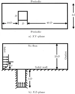
The proposed computational domain and its boundary conditions and the computational grid are shown in Figures 1 and 2, respectively. The Cartesian coordinate system is used in which X is parallel to
the cross ow direction,Y is parallel to the initial jet
ow direction andZis perpendicular to theXY-plane.
Note that the origin of the coordinate system is located on the geometrical center of the jet exit. The cross ow boundary layer thickness used was the same as that used in Ajersch's experimental work ( = 2D),
with a 1/7 power law prole and the jet inlet velocity was considered to be uniform. As shown in Figure 1, a single square cross-section jet was considered in the computational domain. To impose the inuences of the other jets, the periodic boundary condition was used in theZ-direction.
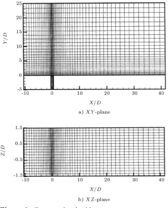
The computational grid used is non-uniform in
Figure 1.
Computational domain and its boundary conditions.Figure 2.
Computational grid.Y-directions, where the grid points are clustered near
the walls, using the following algebraic stretching function [29]:
Y =H
(+ 1) ( 1)f[(+ 1)=( 1)] (1 )
g
[(+ 1)=( 1)]
(1 )+ 1
;
(12) whereand are the metric and the clustering
coe-cient, respectively. Also, grid renement is performed in anX-direction in the cross ow block. That is, the
grid is stretched close to the jet exit and expanded away from it. In the Z-direction, a uniform grid is used in
both blocks. Note that, in the interface of the two blocks, the grid points of the two blocks intersect.
The grid resolution study is performed using dierent grid arrangements, as given in Table 1. Maximum and minimum grid spacings are shown in Table 2 for the two blocks. The third grid in the above mentioned tables is selected for the simulation. An incompressible nite volume method, using an un-steady SIMPLE algorithm and implying a multiblock
Table 1.
Grid arrangements for grid resolution study.Blocks Jet Flow Block Cross Flow Block
Direction
X Y Z X Y ZFirst Grid
7 18 5 80 40 13Second Grid
9 18 7 100 50 19Third grid
11 23 9 120 60 25Fourth Grid
13 28 11 140 70 31staggered grid arrangement, is also used. All spatial terms in the Navier-Stokes equations are discretized using the Power-Law scheme. The Crank-Nicolson scheme is also used for discretization of the temporal terms [30]. Also, the uniform time step of t =
0:01 is considered for time marching up to t = 70
seconds. Each iteration takes nearly 13 seconds. Nearly 12,000 iterations are needed for the convergence and 7,000 iterations are needed for time marching. The simulations are performed using a personal computer with a Pentium VI processor and a 512 mega-bytes memory and no parallel processing has been applied. Note that the time averages of the results are used for investigations.
RESULTS
In this work, the jet behavior in a cross ow, at three dierent velocity ratios, namely, 0.5, 1.0 and 1.5, has been computationally simulated using the LES approach. No temperature dierence between the jet and the cross ow is considered. The jet Reynolds number is taken to be 4700 and, thus, the injected ow is turbulent. Note that, in almost all previous works [7], the cross ow alone has been solved using an existing boundary condition at the jet exit, while, as explained here, it seems to be necessary to solve the ow in the jet channel along with the cross ow, simultaneously.
In Figures 3 to 5, the results of the mean velocity proles of < U >, < V > and < W > versus Y,
for dierent streamwise locations (X=D = 0:0, 1.0,
3.0 and 5.0) at R = 0:5, are shown, respectively.
These results are compared with the experimental and computational results of Ajersch et al. [3].
In Figure 3, the computed mean streamwise velocity proles, < U >, at dierent X-locations, at Z =D= 0:0 are shown forR= 0:5. It should be noted
that the agreement between obtained and experimental results is excellent in comparison with the computa-tional proles of Ajersch et al. However, by increasing
X, there would be a minor deviation between the
present computational data and the experimental work of Ajersch et al., but, even so, the agreements are better than the above mentioned computational results. This may be due to the fact that the grid is stretched near the jet exit. It, therefore, shows that the LES approach has shown its ability to predict the rapid variations near the wall; while the Reynolds Averaged Navier-Stokes (RANS) results of Ajersch et al. have some major diculties in this respect.
In Figure 4, the computed mean vertical velocity proles, < V >, at dierent X-locations, at Z =D =
1:0, are shown for R= 0:5. The agreement between
present and experimental results is not excellent. That is, in Figure 4a, the obtained results show weak agreement with the experimental ones, in comparison
Table 2.
The maximum and minimum grid spacing in each direction for both blocks.Parameter
Minimum Grid Spacing
Maximum Grid Spacing
X Y Z X Y ZFirst Grid
0.1667 0.1667 0.1667 2.0700 1.6784 0.1667Second Grid
0.1250 0.1216 0.1250 1.4931 1.2488 0.1250Third Grid
0.1000 0.0959 0.1000 1.1911 0.9942 0.1000Fourth Grid
0.0833 0.0791 0.0833 0.9994 0.8258 0.0833Figure 3.
<U>-velocity proles ofR= 0:5 at dierentYZ-planes (X=D= 0:0, 1.0, 3.0 and 5.0) atZ =D= 0:0 plane.with the computational results of Ajersch et al. at
Y < 0:7. However, better agreement is obtained at
higherY. In Figures 4b to 4d, the results are improved
and better agreement is obtained. It is shown that, near the jet exit, the rapid variations near the wall, which seem to be reasonable, are, again, predicted by the LES approach. Of course, here, there are not enough existing experimental data with which to compare the authors' results.
In Figure 5, the computed mean spanwise velocity
proles, < W >, at dierent X-locations, atZ =D =
0:5, are shown for R = 0:5. It is also noted that
the agreement between the present proles and the experimental data is relatively good. In Figure 5a, the obtained results show weak agreement with the experimental ones, in comparison with the computa-tional results of Ajersch et al. However, in Figures 5b to 5d, the results are improved and better agreement is obtained atY <0:7. As shown, at the jet exit, the
Figure 4.
<V >-velocity proles ofR= 0:5 at dierentYZ-planes (X=D= 0:0, 1.0, 3.0 and 5.0) atZ =D= 1:0 plane.results is approximately -0.72, while this value is -0.76 from the RANS results of Ajersch et al. Although there are no experimental data with which to compare, from other comparisons, the LES value seems to be closer to the corresponding experimental results.
Generally speaking, the present LES results are extremely close to the existing experimental results. However, in some cases, the RANS simulations show some improvement over the LES. It should be noted that, in the k " model of the RANS simulation,
there are several ow dependent constants that are adjusted and which play the role of improving the results. In the LES, only the Smagorinsky constant could be adjusted, the value of which is obtained from Equation 10. Therefore, the existing small discrepan-cies may be due to the deciendiscrepan-cies of the Smagorinsky SGS model. This model is based on the eddy viscosity assumption and only dissipates the energy, not allowing the backscattering of the energy from the small scales to the large scales. That is to say, it is more dissipative
near the solid walls, but, as can be seen from the above gures, here, this error can be ignored. Of course, using dynamic subgrid scale models, which require more computer time and memory, can improve the accuracy signicantly.
In Figures 6 to 8, the time-mean velocity vectors in three dierent YZ-planes of X=D = 1:0, 3.0 and
5.0, for three respective velocity ratios ofR= 0:5, 1.0
and 1.5, are shown. As the velocity ratio increases, the jet to cross ow momentum ratio increases. This causes the jet to penetrate more into the cross ow. On the other hand, for all three velocity ratios, as the distance at anX-direction from the jet exit increases,
the jet ow detaches more from the wall. Therefore, as expected, at further distances from the jet exit, the Counter Rotating Vortex Pairs (CRVP) get further away from the wall. At the same time, the distance between the CRVP centers in the spanwise direction varies.
-Figure 5.
<W >-velocity proles ofR= 0:5 at dierentYZ-planes (X=D= 0:0, 1.0, 3.0 and 5.0) atZ =D= 0:5 plane.direction from the jet exit increases, the centers of the CRVP get further away from the wall. That is, the CRVP centers in the Y-direction are located at
0.22, 0.49 and 0.65, at X=D = 1:0, 3.0 and 5.0,
respectively. This ow feature could be observed at the higher velocity ratios of Figures 7 and 8. Therefore, the centers are located at Y=D = 0:43, 0.92 and 1.14,
for R = 1:0 and at Y=D = 0:5, 1.03 and 1.38, for R = 1:5 at the corresponding X=D = 1:0, 3.0 and
5.0, respectively. It is concluded that, as the distance from the jet exit increases, theY-position of the CRVP
centers increases at all velocity ratios.
The spanwise distance between the CRVP centers decreases as the distance from the jet exit increases at R = 0:5. These distances are 1.3, 0.73 and 0.71
at X=D = 1:0, 3.0 and 5.0, respectively. However,
at R = 1:0 and 1.5, this ow feature is observed,
except for X=D = 5:0. At R = 1:0, the spanwise
distances between the centers are 1.36, 0.73 and 1.0 and at R = 1:5, these distances are 1.65, 0.92 and
0.98 at the corresponding X=D = 1:0, 3.0 and 5.0,
respectively. This behavior is due to the fact that, at higher velocity ratios, the CRVP expands more and touches the spanwise periodic boundary at a lower X
after the jet exit.
When the velocity ratio is low, the jet ow is bent towards the wall at each side. Thus, only the jet ow will be in contact with the wall. Furthermore, near the jet exit, the jet penetration is negligible and so is its mixing with the cross ow uid. It can be concluded that, in lm cooling applications, the velocity ratio must be low. Of course, there are other parameters, like injection angle and injection geometry etc., which must be optimized. At higher velocity ratios, the cross ow uid comes under the jet ow from each side and pushes it up; therefore, its penetration is considerable. So, in this situation, the jet to cross ow mixing is high and the cross ow will be in contact with the surface.
After the jet enters the cross ow, it becomes very vortical. Actually, highly strong vortical regions, i.e.
Figure 6.
Time-mean velocity vectors in dierent YZ-planes (X=D= 1:0, 3.0 and 5.0) atR= 0:5.the CRVP, will be formed, which will be dissipated far from the jet exit. The main inuence of this vortical motion is to mix the jet with the cross ow. So, in lm cooling applications, it is desirable to decrease such vortical motion by optimizing the velocity ratio and the other eective parameters. On the other hand, in problems such as pollutant dispersion, gas injection
Figure 7.
Time-mean velocity vectors in dierent YZ-planes (X=D= 1:0, 3.0 and 5.0) atR= 1:0.in combustors and the mixing of liquids/gases, the objective is to generate these vortical regions as soon and as strong as possible.
CONCLUSIONS
mul-Figure 8.
Time-mean velocity vectors in dierent YZ-planes (X=D= 1:0, 3.0 and 5.0) atR= 1:5.tiple square cross section jets into a cross ow on a at plate, at three dierent velocity ratios of 0.5, 1.0 and 1.5, are studied, using the LES approach. The LES results are in much better agreement with the existing experimental results, in comparison with the relevant computational results of the RANS approach. After the jet enters the cross ow, it generates counter
rotating vortex pairs, expands and penetrates to the cross ow in theYZ-plane. The results show that:
1. By increasing the velocity ratio, the jet penetration into the cross ow is increased, accompanied by high mixing with the cross ow;
2. After the jet enters the cross ow, it forms highly vortical regions, which are called Counter Rotating Vortex Pairs (CRVP);
3. As the distance in an X-direction from the jet
exit increases, the Y-position of the CRVP centers
increases at all velocity ratios;
4. The spanwise distance between the CRVP centers decreases before the CRVP touches the spanwise periodic boundary;
5. The main inuence of these vortical behaviors is to mix the jet with the cross ow;
6. The CRVP gets stronger, as the velocity ratio increases. Therefore, it is suggested that, in lm cooling applications, low velocity ratio and, inversely, in ows such as pollutant dispersion, gas injection in combustors and the mixing of liquids/gases applications, high velocity ratios, are to be applied.
REFERENCES
1. Andreopoulos, J. \On the structure of jets in a cross-ow", Journal of Fluid Mechanics,
157
, pp 163-197 (1985).2. Lee, S.W., Lee, J.S. and Ro, S.T. \Experimental study on the ow characteristics of streamwise inclined jets in crossow on at plate",Journal of Turbomachinery,
116
, pp 97-105 (1994).3. Ajersch, P., Zhou, J.M., Ketler, S., Salcudean, M. and Gartshore, I.S. \Multiple jets in a crossow: Detailed measurements and numerical simulations", Interna-tional Gas Turbine and Aeroengine Congress and Ex-position, ASME Paper 95-GT-9, Houston, Texas, USA, pp 1-16 (1995).
4. Holdman, J.D. and Walker, R.E. \Mixing of a row of jets with a conned crossow",AIAA Journal,
15
(2), pp 243-249 (1977).5. Hoda, A. and Acharya, S. \Predictions of a lm coolant jet in crossow with dierent turbulence models",
Journal of Turbomachinery,
122
, pp 558-569 (2000). 6. Keimasi, M.R. and Taeibi-Rahni, M. \Numericalsim-ulation of jets in a crossow using dierent turbulence models",AIAA Journal,
39
(12), pp 2268-2277 (2001). 7. Acharya, S., Tyagi, M. and Hoda, A. \Flow and heat transfer predictions for lm cooling", Heat Transfer in Gas Turbine Systems, Annals of the New York Academy of Sciences,934
, pp 110-125 (2001).8. Kapadia, S., Roy, S. and Heidmann, J. \Detached eddy simulation of turbine blade cooling",36th Ther-mophysics Conference, AIAA-2003-3632, Orlando, Florida, USA, pp 1-10 (2003).
9. Hass, W., Rodi, W. and Schonung, B. \The inuence of density dierence between hot and coolant gas on lm cooling by a row of holes: Predictions and experiments", Journal of Turbomachinery,
114
, pp 747-755 (1992).10. Honami, S., Shizawa, T. and Uchiyama, A. \Be-havior of the laterally injected jet in lm cool-ing: Measurements of surface temperature and ve-locity/temperature led within the jet", Journal of Turbomachinery,
116
, pp 106-112 (1994).11. Hassan, I., Findlay, M., Salcudean, M. and Gartshore, I. \Prediction of lm cooling with compound-angle injection using dierent turbulence models", 6th An-nual Conference of the Computational Fluid Dynamics Society of Canada, Quebec, Canada, pp 1-6 (1998). 12. Amer, A.A., Jubran, B.A. and Hamdan, M.A.
\Com-parison of dierent two-equation turbulent models for prediction of lm cooling from two rows of holes",
Numerical Heat Transfer, Part A,
21
, pp 143-162 (1992).13. Thole, K., Gritsch, M., Schulz, A. and Witting, S. \Floweld measurements for lm-cooling holes with expanded exits",Journal of Turbomachinery,
120
, pp 327-336 (1998).14. Schmidt, D.L. and Bogard, D.G. \Pressure gradient eects on lm cooling",International Gas Turbine and Aeroengine Congress and Exposition, ASME Paper 95-GT-18, Houston, Texas, USA, pp 1-8 (1995).
15. Ramezanizadeh, M. and Taeibi-Rahni, M. \Large eddy simulation of three-dimensional cavity ow using Smagorinsky model", First International and Third Biennial Conference of the Iranian Aerospace Society, Sharif University of Technology, Tehran, Iran,
4
, pp 99-106 (2000).16. Ghosal, S. \Mathematical and physical constraints on LES",AIAA, Paper 98-2803, pp 1-13 (1998).
17. Ramezanizadeh, M. and Taeibi-Rahni, M. \Large eddy simulation of a two-dimensional at plate lm-cooling",The Ninth Asian Congress of Fluid Mechan-ics, Isfahan University of Technology, Isfahan, Iran, pp 1-7 (2002).
18. Tafti, D.K., Zhang, X., Huang, W. and Wang, G. \Large-eddy simulations of ow and heat trans-fer in complex three-dimensional multilouvered ns",
ASME Fluids Engineering Division Summer Meeting, FEDSM2000-11325, Boston, Massachusetts, USA, pp 1-18 (2000).
19. Sohankar, A. and Davidson, L. \Large eddy simula-tion of turbulent ow over a square prism by using two subgrid-scale models", 4th International and 8th Annual Conference of Iranian Society of Mechanical Engineers, Sharif University of Technology, Tehran, Iran,
3
, pp 551-558 (2000).20. Iliescu, T. and Fischer, P. \Backscatter in the rational LES model",J. Computers and Fluids,
33
, pp 783-790 (2004).21. Meinke, M., Schroder, W., Krause, E. and Rister, T. \A comparison of second- and sixth-order methods for large-eddy simulations",J. Computers and Fluids,
31
, pp 695-718 (2002).22. Peyret, R.,Handbook of Computational Fluid Mechan-ics, San Diego, Academics Press (1996).
23. Zhang, W. and Chen, Q. \Large eddy simulation of indoor airow with a ltered dynamic subgrid scale model",International Journal of Heat and Mass Transfer,
43
, pp 3219-3231 (2000).24. Pomraning, E. and Rutland, C. \Dynamic one-equation nonviscosity large-eddy simulation model",
AIAA Journal,
40
(4), pp 689-701 (2002).25. Ghia, U., Ghia, K.N. and Shin, C.T. \High-Re solu-tions for incompressible ow, using the Navier-Stokes equations and a multigrid method",J. Comp. Phys.,
387
, pp 387-411 (1982).26. Ramezanizadeh, M., Large Eddy Simulation of Film Cooling in a Turbulent Flow Over a Flat Plate, MSc. Thesis, Aerospace Eng. Dept., Sharif University of Technology, Tehran, I.R. Iran (2000).
27. Zang, Y., Street, R.L. and Kose, J.R. \A dynamic mixed subgrid-scale model and its application to tur-bulent recirculating ows",Phys. Fluids A,
5
(12), pp 3186-3096 (1993).28. Taeibi-Rahni, M. and Ramezanizadeh, M. \Investiga-tion of three-dimensional cavity ow using large eddy simulation", J. Aerospace Science and Technology,
2
(2), pp 1-10 (2005).29. Homann, K.A. and Chiang, S.T. \Computational uid dynamics for engineers",Engineering Education Science,
1
, USA, Chapter 9, pp 470-471 (2000). 30. Versteeg, H.K. and Malalasekara, W.,An Introductionto Computational Fluid Dynamics-The Finite Volume Method, Longman Malaysia, Chapters 5-7, pp 103-167 (1995).