Sharif University of Technology
Scientia IranicaTransactions A: Civil Engineering www.scientiairanica.com
Developing water quality maps of a hyper-saline lake
using spatial interpolation methods
S. Sima
and M. Tajrishy
Department of Civil Engineering, Sharif University of Technology, Tehran, Iran. Received 7 July 2013; received in revised form 27 May 2014; accepted 25 October 2014
KEYWORDS Urmia Lake; Water quality; Interpolation methods; Kriging; Cations; Anions.
Abstract.Urmia Lake, the second largest hyper-saline lake in the world, has experienced a signicant drop in water level during the last decade. This study was designed to examine the water quality of Urmia Lake and to characterize the spatial heterogeneity and temporal changes of the physiochemical parameters between October 2009 and July 2010. Two spatial interpolation methods, Inverse Distance Weighting (IDW) and Ordinary Kriging (OK), were used and compared with each other to derive the spatial distribution of ionic constituents as well as TDS and density along the lake. Results showed that the main dominant cations and anions in Urmia Lake were Na+, Mg++, K+, Ca++, Cl , SO
4 ,
and HCO3, respectively. Although water quality of the lake is homogeneous with depth, it diers between the northern and southern parts. Water quality also varies seasonally, determined by river inows and the lake bathymetry. Moreover, with the present salinity level, salt precipitation is likely in Urmia Lake and is becoming one of the principal factors determining the distribution of solutes within the lake. This study shows that the combined use of temporal and spatial water quality data improves our understanding of complex, large aquatic systems like Urmia Lake.
© 2015 Sharif University of Technology. All rights reserved.
1. Introduction
Lakes are valuable water resources supporting a var-ious range of human activities including agriculture, commerce, transportation, recreation, tourism, and the production of food and energy. They also provide unique habitats for a diverse array of organisms and play a key role in the meteorological conditions of their surrounding environments. Monitoring water quality is crucial to the proper management and restoration of many lakes particularly in large lakes.
Urmia Lake is located in north-west Iran and is the second most saline lake in the world [1]. It is a shallow terminal lake which lies between 37040N
to 38170N latitude and 45E and 46E longitude.
*. Corresponding author. Tel.: +98 21 66164185
E-mail addresses: [email protected] (S. Sima); Tajrishy@ sharif.ir (M. Tajrishy)
Its surface area has been estimated to be 6059 km2
in 1995 [2], but since then it has been declining [3] and was estimated to be only 2366 km2 in August of
2011 [4]. Urmia Lake has been divided by a 15.4 km dike-type causeway which provides road access between the western and eastern provinces (Figure 1). A 1.25 km long opening was left in the causeway to hydraulically connect the northern and southern parts of the lake. Because of its high salinity, Urmia Lake has a low diversity of ora and fauna, and except Artimia Urmiana Salina and some algae species, no other living organisms exist [5]. Urmia Lake has been designated as a Ramsar Convention Site of international importance (since 1971), Biosphere Reserve (since 1976), and a national park and is one of the largest natural biotopes of Artemia in the world [6]. The locations of the four major islands, Kabudan, Arezu, Ashk, and Espir, which are considered as protected areas by the
Figure 1. West Azerbaijan province and Urmia Lake map.
Environmental Protection Organization, are shown in Figure 1.
Upstream river discharges as well as seasonal precipitation are the main sources of the water to this terminal lake, while evaporation is the main water loss. The average surface and ground wa-ter inows to the lake have been estimated to be 5.3 km3/year. The semi-arid local climate of the
region leads to the high evaporation and low pre-cipitation rates. The average volume of evaporation from the lake is estimated to vary between 900 and 1170 mm/year while the average precipitation over the lake is 350 mm/year [2].
In recent years, due to drought and increased demands for agricultural water in the lake's basin, its water level has dropped by more than 7.5 meters below its maximum level (see Figure 2), and large areas of the lake bed have desiccated. Concurrently, the salinity of the lake has risen to more than 300 g/L which has caused the severe disturbances to the lake ecosys-tem [7]. Several factors including climate changes and anthropogenic changes such as dam construction and over exploitation of water in the Urmia basin have inuenced the water quality of Urmia Lake during the past two decades. However, due to the lack of continuous measurements from the physiochemical parameters of the lake, little is known about the spatial and temporal variation of its water quality.
During the past decades, several studies have been performed by dierent organizations on the water quality of Urmia Lake. However, in the majority of
Figure 2. Mean annual water level uctuation of Urmia Lake measured in Golmankhaneh station (depicted by No.1 on Figure 1) from 1967 to 2010.
these studies either the spatial coverage or the temporal frequency of samplings was not adequate enough to achieve a clear understanding of the water quality in Urmia Lake. For instance, West Azerbaijan Regional Water Company regularly gathers samples from the lake shores and interprets the lake chemistry based on them. As other examples, Aazami-Oscoie [8] and Daneshgar and Ashasi [9] studied the water composi-tion of Urmia Lake at the Heidarabd area (Stacomposi-tion 3 in Figure 1) and Sharafkhaneh (Station 2 in Figure 1). However, due to the low water depth and very high salt concentration at the lake shores, the shoreline samples
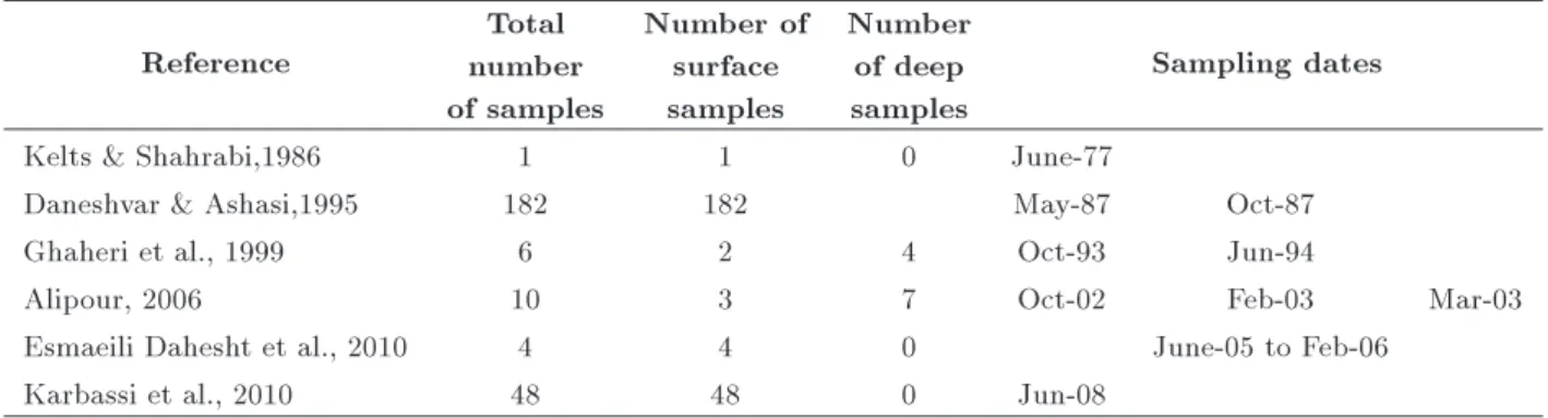
Table 1. Summary of water quality monitoring studies in Urmia Lake. Reference
Total number of samples
Number of surface samples
Number of deep samples
Sampling dates
Kelts & Shahrabi,1986 1 1 0 June-77
Daneshvar & Ashasi,1995 182 182 May-87 Oct-87
Ghaheri et al., 1999 6 2 4 Oct-93 Jun-94
Alipour, 2006 10 3 7 Oct-02 Feb-03 Mar-03
Esmaeili Dahesht et al., 2010 4 4 0 June-05 to Feb-06
Karbassi et al., 2010 48 48 0 Jun-08
are not suitable representatives of whole-lake water quality.
Literature data on Urmia lake water chemistry are summarized in Table 1. In all studies performed before 2000, water quality of the lake was described based on only a few samples and hardly any deep water samples. Many attempts have been made over the past decade to examine the lake water quality using more comprehensive sampling schemes. For example, Alipour [10] studied the hydro-geochemistry of the lake and determined seasonal variation of the major anions and cations based on 10 samples collected at three depths in the western half of the lake. He concluded that Urmia Lake was geochemically uniform in the south and north side of the causeway. Later, Esmaeili Dahesht et al. [11] reported results of the measure-ments of some main water quality parameters of the lake including TDS, chloride, sulfate, magnesium and bicarbonate concentrations based on the two samples from the north, and two samples from the south part of the lake. Subsequently, Karbassi et al. [7] performed a complete water quality analysis based on 48 samples gathered from the lake surface in order to investigate the impacts of desalination on the ecology of Urmia Lake. Besides these studies, few studies was carried out to examine the spatio-temporal variation of Urmia Lake surface temperature (e.g. [12]), which in turn can aect the water chemistry of the lake.
All of these studies are based on datasets col-lected at dierent sites or along track lines occupied during cruises. However, environmental managers often require spatially continuous data over the region of interest to make eective and condent decisions. Spatial interpolation methods can be used to overcome such shortcomings by estimating spatially continuous data from discrete data points [13].
A number of methods have been developed for spatial interpolation in various disciplines including mining engineering [14], meteorology [15-17] and en-vironmental sciences [14,18,19]. A bibliographic re-search carried out by Zhou et al. [20] ranked envi-ronmental sciences as the third highest eld to use spatial interpolation methods. Nevertheless, there
are few studies which have compared dierent in-terpolation methods used to determine water quality maps within lakes. For example, Bellehumeur et al. [21] described a geostatistical technique based on conditional simulations to assess pH values on the Canadian Shield. Nas et al. [22] applied Ordinary Kriging to develop spatial distribution maps of total nitrogen and phosphorus, turbidity, Secchi disk depth and chlorophyll-a over Beysehir Lake. Alc^antara [23] studied turbidity in an Amazon oodplain lake through OK and wavelet analysis. In another study, Murphy et al. [24] compared three interpolation methods com-prising inverse distance weighting, Ordinary Kriging, and a Universal Kriging method to evaluate spatial and vertical distribution of water quality parameters (salinity, water temperature, and dissolved oxygen) in the Chesapeake Bay. They concluded that the Kriging methods generally outperform inverse distance weighting for all parameters and depths. Recently, a study has been performed on the pollution con-trol of three Forks Lake using cluster analysis and inverse distance-weighted interpolation, to determine the spatial distribution of water quality parameters such as pH, NH3-N, total phosphorus, total
nitro-gen, permanganate index, transparency, Total Dis-solved Solids (TDS), DisDis-solved Oxygen (DO), and conductivity [25]. Spatio-temporal changes in the total phosphorus concentrations of the Everglades wetland (Robertson) were assessed using an ordinary Kriging spatial interpolator with an acceptable er-ror [26].
At least 42 dierent spatial interpolation meth-ods have been recognized in various disciplines [27]. Although some methods have been shown to perform better than others, the results appear to be study and site specic, and thus no denite conclusion has been made on which method is the best or most appropriate [24]. Nonetheless, in the eld of en-vironmental sciences, ordinary Kriging and Inverse Distance Weighting (IDW) methods are recognized as the most widely used stochastic and deterministic techniques [27,28].
sea-sonal maps of Urmia Lake water chemistry using spatial interpolation methods. To accomplish this task, water quality data collected during three sampling periods from 2009-2010 were applied. Next, two conventional interpolation techniques, IDW and OK, were employed and compared using cross-validation to nd the most appropriate interpolation scheme for each parameter. Subsequently, applying the proper interpolation tech-nique for each ion, maps of major anions and cations as well as density were developed. Finally, spatial and temporal variations of ion concentrations in Urmia Lake were examined using the retrieved maps and compared with previous water quality studies.
This is the rst comprehensive limnological in-vestigation to present spatial distribution of water quality parameters in Urmia Lake and contains several unique aspects, such as its application to a large hyper-saline lake, its reasonably adequate ability to compare parameters on an inter-annual scale, and its comparison of techniques currently being considered for management applications. This study provides insights into the development of water quality data of adequate spatial and temporal resolution to be used for validation purpose in hydrodynamic models. Furthermore, determining water quality distribution along Lake Urmia and its potential eects on the lake fauna can help managers to make informed decisions on suitable restoration plans.
2. Methodology 2.1. Sampling
Selection of sampling points on the lake surface was made using a topographic map with a scale of 1:250,000 on which a 1010 km rectangular network was designed to cover the entire lake (Figure 1). However, as a result of signicant water level decline, vast parts of the lake shores have desiccated and been altered into muddy surfaces covered by saline sediments. It is awkward to take samples from these inshore regions (areas of about 1 m water depth) either by motorboat or hiking. Moreover, water level drop and resultant salt precipitation has caused the formation of salt mounds in some parts of the lake bed which halts navigation of boats. Therefore, it was not feasible to exactly track the designed, regular network. Instead, through cruising along the accessible parts of the lake, samples were collected approximately at 10 km intervals and the locations were recorded using a GPS recorder. The spatial distribution of sampling locations and the depth of samples are shown in Figure 3.
We considered seasonal frequency for sampling between October 2009 and to July 2010. Nonetheless, during the cold season, December to March, harsh climate conditions trigger wind-driven currents along the lake which prohibits the safe use of motor boats.
Figure 3. Sampling locations along Urmia Lake, where S, M, D and VD represent surface (0.5 m), middle (1 m), deep (1.5 m) and very deep samples (> 2:5 m).
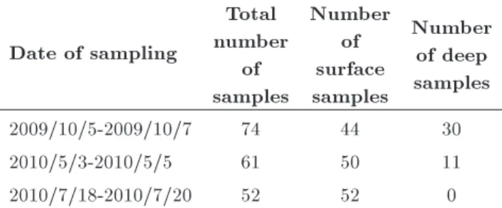
Table 2. Number and location of sampling points.
Date of sampling
Total number
of samples
Number of surface samples
Number of deep samples
2009/10/5-2009/10/7 74 44 30
2010/5/3-2010/5/5 61 50 11
2010/7/18-2010/7/20 52 52 0
Therefore, excluding the winter, samplings were carried out during the three periods from October 2009 to July 2010 (Table 2).
Most of the samples were taken from the lake surface (0.5 m depth) with the objective of determining the spatial distribution of water quality parameters within the entire lake. In addition, during the two rst sampling periods, several samples were collected from dierent depths of the lake to examine the vertical distribution of water quality parameters. Information about the number and depth of samples in each period can be found in Table 2.
2.2. Chemical analyses
All collected samples were transferred to the laboratory and analyzed for various physiochemical parameters according to Standard Method protocols [29]. Tem-perature, pH, and density of the water samples were measured at the sampling sites using a thermometer, a digital pH meter (Hach pH meter) and a density meter (Anton Paar: DMA 35N), respectively. Total Dissolved Solids (TDS) and Total Suspended Solids (TSS) were gravimetrically determined at 105 110C.
Chloride concentration was determined by silver ni-trate (AgNO3) titration, using potassium chromate
(K2CrO4) solution as the indicator. Sodium and
potassium were measured by ame photometry, while the concentration of Ca++ and Mg++ were obtained
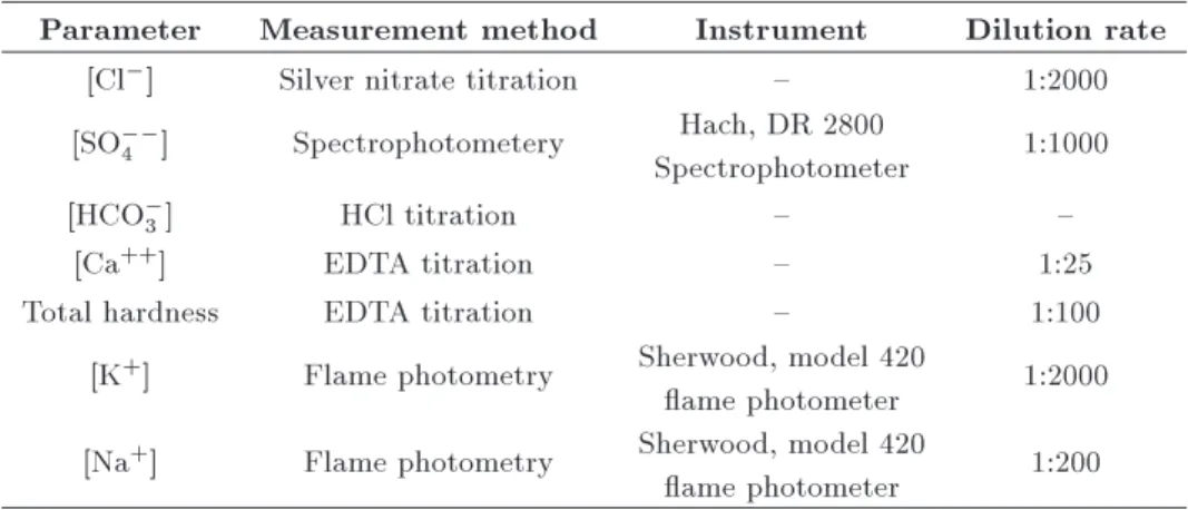
Table 3. Dilution rate of Urmia Lake water samples in physico-chemical tests. Parameter Measurement method Instrument Dilution rate
[Cl ] Silver nitrate titration { 1:2000
[SO4 ] Spectrophotometery Hach, DR 2800
Spectrophotometer 1:1000
[HCO3] HCl titration { {
[Ca++] EDTA titration { 1:25
Total hardness EDTA titration { 1:100
[K+] Flame photometry Sherwood, model 420
ame photometer 1:2000 [Na+] Flame photometry Sherwood, model 420
ame photometer 1:200
through EDTA titration and HCO3 by acid titration. Concentration of SO4 was also determined using a Hach DR2000 spectrophotometer. As the concentra-tion of the lake anions and caconcentra-tions was high, it was necessary to dilute samples with super pure water. The applied dilution rates for each test are presented in Table 3.
2.3. Developing water quality maps 2.3.1. Interpolation methods
To visualize the spatial patterns of the water quality data within Urmia Lake, two spatial interpolation methods, IDW and OK, were applied. Estimations of nearly all spatial interpolation methods can be represented as weighted averages of sampled data as:
^z(x0) = n
X
i=1
wi:z(xi); (1)
where ^z is the estimated value of an attribute at the point of interest x0, z is the observed value at the
sampled point xi, wi is the weight assigned to the
sampled point, and n represents the number of sampled points used for the estimation [19].
Inverse Distance Weighting (IDW) is a determin-istic and exact interpolation method which requires few decision parameters. IDW is a robust method that estimates the values of an attribute at unsampled points using a linear combination of values at sampled points weighted by an inverse function of the distance from the point of interest to the sampled points. The assumption is that sampled points closer to the un-sampled point are more similar to it than those further away in their values [30]. In IDW, weights can be expressed as:
wi= 1=d P i
Pn
i=11=dPi ; (2)
where:
n
X
i=1
wi = 1;
in which di is the distance between sampled point, xi,
and the estimated point, x0; p is a power parameter,
and n represents the number of sampled points used for the estimation. The accuracy of IDW is mainly determined by the value of the power parameter and search radius [31]. Weights diminish as the distance increases, especially when the value of the power parameter increases. The Inverse Distance Weighting method (IDW) works best with a limited sample size and random data points. Further details on the IDW method can be found in Ashraf et al. [32]. Although the choice of power parameter and neighborhood size is ar-bitrary [19], they signicantly aect the accuracy of the resulting estimations. They can also be determined on the basis of error measurement [33]. The smoothness of the estimated surface increases as the power parameter increases. The most popular choice of power is 2 [34]. In our case, we tested IDW with powers of 1 and 2, and various neighboring radius to optimize the variables of the inverse distance function for various water quality constituents during each sampling period. Selection of optimum variables was performed based on the results of the Leave-One-Out Cross Validation (LOOCV).
Kriging is considered the best linear unbiased interpolation method to estimate the value of region-alized variables at an unsampled location. Kriging assigns weights according to a stochastic function which is calculated based upon the spatial correlation structure of the observations [31]. Kriging makes use of Regionalized Variable Theory (RVT), which postulates that variation is best described by a stochastic surface and denes the value of the random variable Z at x as: Z(x) = m(x) + "0+ "00; (3)
with x representing a generic spatial location assumed to vary continuously over some domain of interest, m structural (deterministic) component, "0 the spatially
correlated random component, and "00spatially
uncor-related random (noise) component.
In Kriging, weights are optimized based on the true spatial structure of the parameter throughout the
region of interest, which is unknown. Semivariogram function is used to estimate the actual spatial structure of the parameter within the study area from the spatial structure of the observations. Weights are then obtained by solving the system of equations:
n
X
i=1
w(i):(xi; xj) + ' = (xj; x0) for all j; (4)
n
X
i=1
wi= 1; (5)
where (xi; xj) represents the value of the
semivari-ogram function for the distance between the points xi and xj, (xj; x0) is the value for the distance
between xj and the estimated location x0, and ' is
the Lagrange parameter. The semivariogram function is derived by tting a semivariogram model to the empirical semivariogram, which can be calculated for all distances h by solving:
^(h) = 2n1
n
X
i=1
(z(xi) z(xi+ h))2: (6)
Several semivariogram models are available and com-monly used to estimate semivariograms based on sam-pled data (e.g. spherical, exponential, linear, Gaussian, power, circular) [35,36].
Kriging can be classied into three types of Simple Kriging (SK), Ordinary Kriging [37], and Universal Kriging (UK). SK assumes a known constant trend, OK assumes an unknown constant trend, and UK assumes a general polynomial trend model. Amongst the dierent types of Krigings, OK has been most commonly applied in environmental studies [38], and as in Poon et al. [28,37]. OK can be represented with Eq. (3), but with no covariates m(x). The OK approach thus contains just the spatially correlated random component, "0, and the noise term, "00,
account-ing for all of the spatial variation in the observations. For more detailed explanation of the Kriging method see [39].
Creutin and Obled [40] discussed that, for low-to medium-density networks, Kriging performed better results than simple weighting methods. However, when the sampling network is dense enough, most interpolation techniques produce similar results [14]. In such high density networks, Kriging is not consid-erably superior to simpler methods, such as IDW [41]. Consequently, improvements in prediction cannot be obtained by applying more sophisticated methods, but rather by gathering more useful and high quality data [42].
In this study, IDW and OK were applied to derive the spatial distribution of ionic constituents, TDS, and density within Urmia Lake. For IDW, two powers (1
and 2) and ve neighborhood radii (20, 25, 30, 35 and 40 km) were tested and compared through cross-validation to nd the optimum scheme. Similarly for OK, dierent types of semivariogram models including spherical, exponential, linear and Gaussian were exam-ined. Then, proper IDW scheme was compared to the OK scheme with appropriate semivariogram using the performance criteria calculated in the cross-validation process.
2.3.2. Evaluation of interpolation techniques
The performance of each of the applied interpolation techniques was evaluated using the cross-validation method, originally proposed by Seaman [43]. In implementing cross-validation, the sample value of a given location is temporarily discarded from the sample dataset, and the interpolation was performed using the remaining samples to generate an estimate at the location of the removed value. This procedure was then repeated for each sample in a data set and the error between the true value and the estimated value was assessed in each run [44].
In this study, cross-validation (LOOCV) was implemented using GS+ Geostatistics for the
Envi-ronmental sciences version 5.1.1. Several performance measures were calculated during the cross-validation procedure in GS+ in order to evaluate the accuracy
of the estimations. Regression coecient between estimated and actual values, Standard Error (SE) of the regression coecient which is equal to Root Mean Squared Error (RMSE), the coecient of determina-tion (R2), and Standard Error of Prediction (SEP) were
used. As the values of the regression coecient and R2 approach one and values of SE and SEP become
smaller, the accuracy of estimation improves [45]. The RMSE and SEP measures are dened as:
RMSE = v u u t 1 n n X i=1
(^zi zi)2; (7)
SEP = SDp(1 R2); (8)
where ^zi and zi are the predicted and observed sample
values, respectively, and n is the total number of samples, and SD is the standard deviation of the actual data.
Among calculated accuracy criteria, RMSE was primarily used to assess the results of cross-validation, while the regression coecient and R2 were used as
supplementary measures. RMSE is thought to be amongst the best overall measures of model perfor-mance, as it summarizes the mean dierence between the units of observed and predicted values [46].
In this study, the described performance measures were applied to: (1) compare dierent IDW schemes, 2) select the optimum semivariogram model for OK,
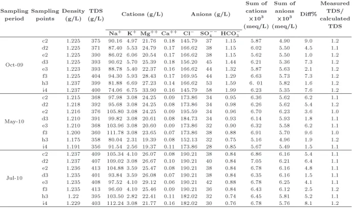
Table 4. Results of water quality analysis for outstanding surface samples during the three samplings in Urmia Lake.
Sampling period
Sampling points
Density (g/L)
TDS
(g/L) Cations (g/L) Anions (g/L)
Sum of cations 103
(meq/L)
Sum of anions 103
(meq/L) Di%
Measured TDS/ calculated
TDS Na+ K+ Mg++ Ca++ Cl SO
4 HCO3
Oct-09
c2 1.225 375 90.16 4.97 21.76 0.18 145.79 37 1.15 5.87 4.90 9.0 1.2 d2 1.225 371 87.40 5.53 24.79 0.17 166.62 38 1.15 6.02 5.50 4.5 1.1 e2 1.225 390 86.02 6.06 20.54 0.17 166.62 38 1.15 5.62 5.50 1.0 1.2 d3 1.225 393 90.62 5.70 25.39 0.18 156.20 45 1.44 6.21 5.36 7.3 1.2 e3 1.223 393 88.78 5.40 22.37 0.16 166.62 44 1.32 5.87 5.63 2.1 1.2 f3 1.225 404 94.30 5.93 28.43 0.17 169.95 44 1.29 6.63 5.73 7.3 1.2 h3 1.237 399 81.88 6.69 27.23 0.14 166.62 53 1.59 6. 01 5.82 1.6 1.2 i4 1.237 400 74.06 6.75 33.90 0.16 145.79 58 1.99 6.23 5.35 7.6 1.2
May-10
c2 1.215 368 97.98 3.08 24.25 0.09 173.86 34 0.95 6.36 5.62 6.2 1.1 d2 1.218 392 95.68 3.08 24.25 0.08 173.86 34 0.98 6.26 5.62 5.4 1.2 e2 1.216 376 105.80 3.08 24.25 0.09 195.59 34 0.96 6.70 6.23 3.6 1.0 d3 1.210 391 99.82 3.08 20.61 0.08 184.73 34 0.93 6.14 5.93 1.8 1.1 e3 1.210 368 103.96 3.08 20.60 0.09 173.86 32 0.90 6.32 5.58 6.2 1.1 f3 1.200 360 111.78 3.08 23.65 0.07 173.86 38 0.88 6.91 5.70 9.6 1.0 h3 1.175 358 80.04 2.31 19.39 0.08 152.13 32 0.75 5.16 4.96 1.9 1.2 i4 1.191 356 91.54 2.56 19.37 0.11 173.86 28 0.85 5.67 5.49 1.5 1.1
Jul-10
c2 1.237 409 105.34 4.10 26.07 0.08 190.21 38 0.84 6.86 6.16 5.4 1.1 d2 1.237 407 109.02 3.08 26.67 0.10 190.21 40 0.84 7.05 6.21 6.4 1.1 e2 1.236 413 104.88 3.59 25.47 0.08 190.21 38 0.84 6.78 6.16 4.8 1.1 d3 1.235 401 93.84 3.59 26.08 0.07 190.21 38 0.84 6.35 6.16 1.5 1.1 e3 1.235 408 97.52 4.10 29.12 0.06 190.21 42 0.88 6.78 6.25 4.1 1.1 f3 1.235 413 96.60 4.10 25.46 0.09 190.21 36 0.84 6.43 6.12 2.5 1.2 h3 1.22 395 103.50 2.82 22.41 0.11 182.02 32 0.74 6.45 5.81 5.2 1.1 i4 1.229 403 112.24 3.08 21.77 0.16 182.02 30 0.76 6.78 5.76 8.1 1.2
and (3) compare between the most appropriate IDW and OK schemes.
3. Results and discussion
3.1. Results of water quality analysis 3.1.1. Water quality data
Results of the water quality analysis for eight surface samples from dierent parts of the lake are tabulated in Table 4. As there were a large number of samples, data for nominated samples from dierent regions of the lake (samples c2, d2, e2, c3, and d3 in the north;
f3 in the middle, near the causeway's opening; h4 and
i4in the south of the lake) are presented (see sampling
grid in Figure 1). Moreover, results of the lake water temperature and density analyses at various depths during May 2010 are presented in Table 5.
3.1.2. Checking for correctness of analysis
To control the correctness of chemical analyses, ion balance of each sample as well as its TDS ratio was checked according to the Standard Methods [29]. As described in the following sections, the Standard Methods correctness criteria were met in all of the chemical analyses. The anion and cation sums, when expressed as milli-equivalents per liter (meq/L), must approximately balance. The balance is checked based upon the percentage dierence (Di) which is dened as follows:
Di = P
Cations PAnions P
Cations +PAnions 100: (9)
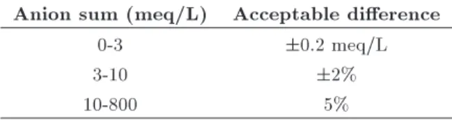
Regarding the concentration of total anions, Di should meet the typical criteria for acceptance of the ion bal-ance check (Table 6). Owing to the high concentration of ionic constituents in Urmia Lake (anion sum=5000-6000 meq/L), the calculated dierences fall beyond the criteria advised by [29]. Consequently, the maximum acceptable dierence was considered to be 10%. The percent dierence between anions and cations was calculated for all the samples, and acceptable balances amongst anions and cations were observed (Table 4).
To perform TDS check, the ratio of measured TDS to the calculated TDS, which is the sum of con-centrations of major anionic and cationic constituents (in milligrams per liter), should fall between 1 and 1.2. If the measured value is less than the calcu-lated one, the higher ion sum and measured values were considered suspicious and the sample should be reanalyzed. If the measured TDS concentration is more than 20% higher than the calculated one, the low ion sum is doubtful and selected constituents should be reanalyzed. TDS control was done for all 185 samples and the over range samples were reanalyzed.
3.2. Validation of the spatial interpolation methods
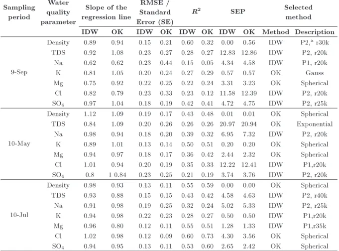
For those water quality parameters of the lake which OK outperforms IDW methods, the optimum tted variogram is illustrated in Figure 4. Table 7 also summarizes the comparison results for the major an-ions and catan-ions, TDS, and density during the three
Figure 4. Experimental and tted variograms for some water quality parameters of Urmia Lake. Table 5. Temperature and density of Urmia Lake water at various depths during May 2010.
Location Sampling
depth (m) Date Time Tair(C) Tw (C) (g/cm
3) pH
North of the causeway
0.5
3-May-10 12:53 16.4
17.8 1.20 7.4
1.5 17.8 1.21 7.3
3 17.7 1.21 7.3
Northeast 0.5 3-May-10 13:10 1 6.1 17.6 1.20 7.3
2 17.6 1.21 7.4
North-deep water
0.5
3-May-10 14:00 1 9.1 16.9 1.22 7.3
4 16.9 1.22 7.3
6 16.9 1.22 7.3
South of the causeway
0.5 3-May-10 15:50 1 5.8 18.0 1.20 7.5
2 18.8 1.21 7.4
South 0.5 5-May-10 11:00 1 7.7 18.7 1.22 7.4
2 18.5 1.22 7.4
South-near the islands
0.5 5-May-10 11:20 1 8.3 19.9 1.21 7.4
1.5 19.4 1.21 7.4
South west 2 5-May-10 12:00 1 9.5 19.2 1.18 7.6
2.5 19.4 1.21 7.4
Table 6. Acceptable dierence between anions and cations in common water and wastewater samples (APHA, 1998).
Anion sum (meq/L) Acceptable dierence
0-3 0:2 meq/L
3-10 2%
10-800 5%
sampling periods. The optimum semi-variogram mod-els show that for all elements, the ranges are higher than 20 km. This means that a 20 km sampling design is suitable to capture the spatial variation in the lake water chemistry. Moreover, comparing the semi-variogram models of K+and Mg++between September
2009 and May 2010, the apparent shorter ranges for spring are because of the freshwater inows to the
Table 7. Comparison of the proper IDW and OK interpolation scheme for the seven water quality parameters of Urmia Lake during the three sampling periods.
Sampling period
Water quality parameter
Slope of the regression line
RMSE / Standard Error (SE)
R2 SEP Selected
method
IDW OK IDW OK IDW OK IDW OK Method Description
9-Sep
Density 0.89 0.94 0.15 0.21 0.60 0.32 0.00 0.56 IDW P2,ar30k
TDS 0.92 1.08 0.23 0.27 0.28 0.27 12.83 12.86 IDW P2, r20k Na 0.62 0.62 0.23 0.44 0.15 0.05 4.34 4.58 IDW P1, r20k
K 0.81 1.05 0.20 0.24 0.27 0.29 0.57 0.57 OK Gauss
Mg 0.75 0.92 0.22 0.25 0.22 0.24 3.31 3.23 OK Spherical Cl 0.82 0.79 0.23 0.33 0.23 0.12 11.58 12.39 IDW P2, r20k SO4 0.97 1.04 0.18 0.19 0.42 0.41 4.72 4.75 IDW P2, r25k
10-May
Density 1.12 1.09 0.19 0.17 0.43 0.48 0.01 0.01 OK Spherical TDS 0.84 1.09 0.20 0.26 0.26 0.26 20.97 20.94 OK Exponential
Na 0.98 0.94 0.18 0.20 0.39 0.32 6.95 7.32 IDW P2, r20k K 0.89 1.01 0.13 0.14 0.50 0.51 0.20 0.20 OK Spherical Mg 0.94 0.97 0.18 0.17 0.36 0.42 2.44 2.32 OK Spherical Cl 1.01 0.94 0.20 0.19 0.35 0.33 12.22 12.41 IDW P1,r20k SO4 0.8 1 0.84 0.23 0.25 0.21 0.19 3.74 3.76 IDW P2, r20k
10-Jul
Density 0.98 0.93 0.13 0.11 0.55 0.59 0.00 0.00 OK Spherical TDS 0.93 0.88 0.15 0.15 0.43 0.42 4.58 4.63 IDW P2, r40k Na 0.91 0.98 0.19 0.25 0.32 0.24 5.02 5.33 IDW P2, r25k K 0.94 0.98 0.22 0.23 0.28 0.27 0.50 0.50 IDW P1,r20k Mg 0.96 0.80 0.12 0.11 0.55 0.51 1.28 1.33 IDW P1,r35k Cl 1.02 0.98 0.12 0.09 0.60 0.73 4.30 3.56 OK Spherical SO4 0.94 0.95 0.13 0.11 0.53 0.60 2.65 2.42 OK Spherical aP and R represent the optimum power and neighborhood radius (in terms of km) for IDW method, respectively. For OK the superior semi-variogram models and their parameters are mentioned.
lake. Therefore, if a coarser sampling network is chosen for each constituent, the sampling distance should be reduced for the spring samples.
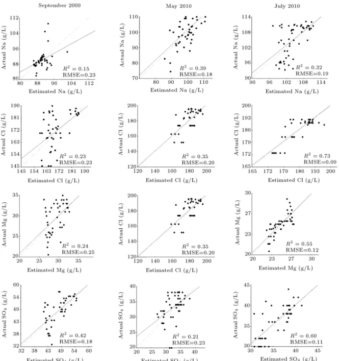
The last two columns of the Table 7 show the superior interpolation method and related parameters applied to derive water quality maps. The cross-validation graphs for all ionic constituents, TDS and density are also displayed in Figure 5. Although it is important to have independent measurements to validate the prediction results [47], the limited number of water quality samples along the large areal extent of the lake inhibited us from dividing samples to the calibration and validation sets. Instead, the LOOCV approach was used to compare the interpolation mod-els. Hence, adding to the number of samples can help to improve the validation procedure of the models based on independent data.
3.3. Ionic composition of the lake
According to the water quality analysis, Na+, Mg++,
K+, and Ca++ are the main cations while Cl , SO 4 ,
and HCO3 are the dominant anions. Stumm and Mor-gan [48] noted that, in freshwater and marine systems,
predominant cations and anions appear in the following order of dominance: Ca++ >Mg++ >Na+ >K+,
HCO3 >SO4 >Cl , Na+ >Mg++ > Ca++ >K+,
and Cl >SO4 >HCO3, respectively. Consequently, the dominant ions of Urmia Lake match with that of typical sea waters, except for the potassium ion concentration which exceeds the calcium concentration in the lake.
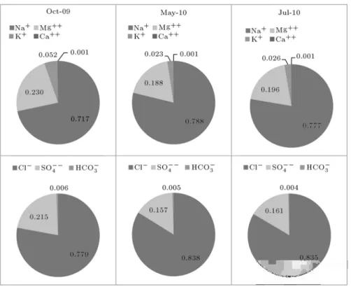
Ionic compositions of Urmia Lake during the three sampling periods were calculated based on the average values of the anions and cations along the lake surface (Figure 6). The lake water comprises of 72-84% sodium and chloride, 15-23% magnesium and sulfate ions, 2-5% potassium, and less than 1% calcium and bicarbonate ions. Moreover, the ionic composition of the lake does not change noticeably between the northern and southern parts. Furthermore, no signicant temporal variation in the ionic composition was recognized. 3.4. Spatio-temporal variation of water quality
parameters
After selection of the proper interpolation methods for each individual parameter, nal maps were created
Figure 5. Validation of the predicted ionic concentrations; TDS and density of Urmia Lake water during the three samplings between October 2009 and July 2010.
using the software ILWIS 3.3 [49]. Distribution of major cations (Na+, Mg++ and K+) and anions (Cl ,
SO4 ) as well as density and TDS in Urmia Lake during October 2009, May, and July 2010 are displayed in Figures 7 and 8. The minimum, maximum, average, and standard deviation of each parameter are also presented.
In terms of spatial variation, three dierent zones can be distinguished: (1) lake shores, (2) the northern part, and (3) the southern part. The spatial distribu-tion of anions and cadistribu-tions along the lake is principally aected by the volume and direction of rivers inow to lake as well as the bathymetry. Other possible factors
such as wind and internal currents can also play a minor role [50].
Generally, the lake shores can be distinguished by having higher concentrations for nearly all ionic constituents during the three sampling periods. In October 2009, for all water quality parameters, the northern part of the lake had lower concentrations than the southern part. Since the rivers inow during this time of the year is minimal, the spatial distribution of anions and cations is most likely determined by the lake bathymetry. Therefore, deeper parts of the lake in the center of the northern and southern section seem to have lower solute concentrations. Moreover,
Figure 6. Ionic composition of Urmia Lake during three samplings.
since the southern section of the lake is shallower, deepening towards the north [10], concentrations of all ions decrease spatially from the south to the north. The same spatial pattern was also observed for density and TDS.
In May 2010, when the lake level was at its maximum (Figure 9), rivers discharge had a more profound eect than topography in determining the spatial pattern of Urmia Lake water chemistry. As most of the freshwater inputs to the lake are from the Shahar Chay River in the west, the anion and cation concentrations in the south decline signicantly, so that the northern section becomes denser (see Figure 7). Furthermore, standard deviation (Std. dev.) of the sodium and chloride ions as well as the density is highest in May, indicating a wide range of values resulting from the dierence between the fresh water and saline water chemistry.
In July 2010, both the rivers discharge and topography played roles in the distribution of ionic constituents along the lake. However, the role of rivers inow was moderate. For all ions except sodium, the southern section remains slightly more dilute compared to the north. Density and TDS are nearly evenly distributed along the lake surface.
Additionally, analysis of the deep samples (from the depths of 1.5, 2, and 3 meters) collected in May 2010 (Table 5) revealed that the lake was not stratied thermally and dierences in the concentrations of ionic constituents with depth are negligible. Since the lake is not stratied during the spring, when the maximum
density dierence is expected because of the freshwater inows to the lake, homogeneous distribution of anions and cations with depth can be taken for granted during all seasons.
Temporally, sodium and chloride concentrations constantly increased from October 2009 to July 2010. In contrast, maximum concentrations of sulfate and magnesium ions were observed in October 2009. In May 2010, concurrent with the rise in water level, concentrations of Mg++ and SO
4 decreased. Then,
following the water level drop in July 2010, their concentrations increased slightly. Similar temporal variations were evident for potassium. Maximum values of TDS and density were observed in October 2009. In May 2010, as a result of increased rivers inow (Figure 5), the lake becomes diluted in terms of TDS and density. From May to July 2010, the average con-centrations of all ionic constituents increased, leading to an increase in the density and TDS of Urmia Lake. This can be inferred by the water level drop of about 25 cm, which is probably due to the limited river inows and increased evaporation.
In October 2009, Na+and Cl were the dominant
cation and anion, respectively (Figure 4). Na+ and
Cl were lower in the next two sampling periods, while Mg++ and SO
4 were at their maximum
con-centrations. This is likely due to the salt dissolu-tion/precipitation mechanism in Urmia Lake. How-ever, in order to condently discuss the roots of such variation, information about the mineralogy of the lake sediment is required. However, such information could
Figure 7. Map of major ions concentration in Lake Urmia during October 2009, May and July 2010.
not be found for Urmia Lake, and investigation of lake sedimentation and dissolution mechanisms is beyond the scope of this study. Nevertheless, this represents a gap in knowledge that should be further addressed in order to improve our current understanding about the chemistry of Urmia Lake.
3.4.1. Comparison to previous studies
To compare the results of the current work with the previous water quality studies, two aspects were considered: the spatial distribution of parameters, and
the average salinity variation. For comparison of the spatial patterns of ionic constituents along the lake, the studies of Alipour [10] and Karbassi et al. [7] were used (Table 1). Although both studies relied on discontinuous data of the lake ionic constituents, there is spatially sucient data of the lake chemistry to be compared with the extracted water quality maps from this work.
Alipour [10] presented distributions of K+ and
Na+ concentrations in the western half of the lake in
Figure 8. Spatial distribution of density and TDS within Urmia Lake.
Figure 9. Water level uctuation in Urmia Lake between October 2009 and July 2010.
the lake was reported to be more concentrated than the northern part. The potassium and sodium maps derived from our study in October 2009 show the same pattern.
Based on the study of Karbassi et al. [7], samples collected in June 2008 show that the average concen-tration of Mg++, K+, Cl , and SO
4 ions in north
are higher than in the south. Na+ concentrations in
the interior part of the lake, in both the southern and northern sections, had the lowest concentrations. Their results are consistent with our ndings from July 2010. To examine the long term water quality variation of Urmia Lake, TDS was used as a water quality indicator. TDS has been measured in nearly all water quality studies, and most samplings have been per-formed between the summer and autumn. Therefore, the summer and autumn samples from various studies were used for comparison.
From Figure 7 it can be seen that TDS levels
Figure 10. TDS and water level variations in Urmia Lake between 1977 and 2010 from several water quality studies.
of the lake have steadily increased between 1977 and 2010, doubling from 1977 to 2010. This constant increase in the lake salinity is due to the negative water balance since 1977 (Figure 10). However, in the coming years, this growing trend will be ceased since the lake is already supersaturated with respect to some salts, mainly halite [7].
We also compared results with results of the hydrodynamic models developed for Urmia Lake. His-torically, several attempts have been made to quantify Urmia Lake hydrodynamics using 2D models [51-55]). Most recently, Zeinoddini et al. [50] investigated ow patterns and salinity distribution along the lake surface in the period from 1994 to 2002 using a 3D hydrodynamic model. They stated that their 3D model is superior to 2D models since it considers vertical variations in velocity and ow. Based on their results, wind was recognized as the dominant climatic factor aecting water ow regime in the lake. However, it has a relatively minor eect on the salinity condition of the lake (less than 4%). On the other hand, river discharge, evaporation, and rainfall were found to be the prevailing hydrological parameters aecting salinity distribution in the lake [50]. They found that in the spring, due to rivers inow to the southern sections, the north part had a higher density and salinity. Whereas, in summer and autumn, interior parts of the lake have higher salinity compared to the shores, which are aected by the rivers inow. During winter months, the lake is almost homogeneous in terms of salinity [50,53]. However, apart from similarities in the temporal variation of the lake salinity, our ndings contradict the results of the hydrodynamic models in several aspects. First, in summer and autumn, the northern part is slightly less saline than the south. Second, the salinity concentration is generally lower in interior parts of the lake than along the shores. The dierences arise from the variations in the lake condition during the recent
Figure 11. Variations of upstream rivers inow to Urmia Lake during 1982-2008.
Figure 12. Landsat satellite images of Urmia Lake [4]. The lake boundary change between 1969 and 2011 is demonstrated.
decade, including a remarkable decline in freshwater inows (Figure 11), as well as the substantial drop in water level (more than 2 meters). There has been signicant retreat from the lake shores, so that vast areas of the shore have converted to salt-covered, muddy wastelands which absorb freshwater inows and prohibit them from entering the lake (see Figure 12). Therefore, except some parts where the river mouth has not yet been dried (e.g. Shahar Chay mouth in the west), river discharges cannot considerably alter the salinity pattern within the lake. Taking into account the present situation of the lake, salinity is mainly determined by the lake bathymetry rather than
the river inows, particularly in dry seasons. Thus, interior, deep parts of the lake have lower salinity concentrations compared to the shores. Likewise, since the northern part is deeper than the south, when river inows from the south are restricted, the southern section remains denser.
4. Conclusions
Urmia Lake, which is of national and international importance, has experienced a dramatic water level decline in recent years. This negative water balance has strongly inuenced the salt content within the lake. The objective of this study was to characterize the spatial heterogeneity and temporal change of phys-iochemical parameters within Urmia Lake by means of two spatial interpolation methods, IDW and OK. The ionic constituents of Urmia Lake were measured in 185 samples during three sampling periods from October 2009 to July 2010. Then, based on the appropriate spatial interpolation scheme, water quality maps were developed and used to examine the spatial and temporal variations. The main conclusions of this study are:
The dominant ionic composition of Urmia Lake is as follows; Cl , Na+, SO
4 , Mg++, K+, HCO3
and Ca++, respectively. No signicant spatial and
temporal variations in the ionic composition of the lake were recognized.
Comparison of ionic constituents using the IDW and OK interpolation techniques indicates that the superior method diers between parameters and season. Thus, no general method can be applied to individual water quality parameters.
Monitoring temporal uctuations of the major ions showed that the lowest concentrations of sodium and chloride occurred in October 2009 while the maximum values were observed in July 2010. In contrast, maximum and minimum concentrations of sulfate and magnesium occurred in October 2009 and May 2010, respectively.
Rivers discharge, bathymetry, and salt precipita-tion/dissolution mechanism were recognized as the three fundamental factors controlling the spatial pattern of Urmia Lake chemistry. During the spring, the chemical distribution patterns along the lake are dominated by inows from the surrounding rivers, while in dry seasons, the role of the other two factors becomes stronger.
It was found that the lake density varies between 1.18 and 1.24 g/cm3 depending on the region and
season, which is much higher than the density of open ocean water. Although freshwater inows during spring may dilute the lake water in the short
term, they are not signicant enough to stabilize the lake in this condition.
The salinity level of the lake has been consistently increasing since 1977, so that TDS concentration has been doubled from 1977 to 2010. Historically, the salinity concentration of the lake is highly dependent upon the lake water level, and currently the lake is nearly saturated with several minerals.
Results of the previous hydrodynamic models cannot be applied to investigate the ow and salinity patterns of the lake since they relied on the water quality data with inadequate spatial and temporal dis-tribution. To have a clear and sucient understanding of the lake dynamics, models should be updated and validated based on currently available water quality data.
To improve predictions of the spatial distribution of the lake chemistry, we suggest considering the lake bathymetry as a covariate through using hybrid interpolation methods such as regression-Kriging [56] or Linear mixed models [57]. Moreover, investigation of the eect of considering the temporal correlation between water quality parameters through the spatial interpolation on the quality of predictions is recom-mended. It is also crucial to investigate salt precipi-tation/dissolution mechanism in Urmia Lake as one of the foremost factors inuencing its chemistry. Inclusion of such mechanisms in the spatio-temporal variations of ionic constituents requires information about the mineralogy of the lake sediments. However, long term monitoring of the lake sediment is currently lacking but highly recommended.
This study demonstrates the successful appli-cation of interpolation techniques to analyze spatio-temporal variation of lakes water chemistry. This shows a great potential to increase the understanding of water quality variation in complex aquatic systems. Results of such research can assist in the implementa-tion of adaptive management and restoraimplementa-tion projects in large lakes by providing new insights and information to managers.
Acknowledgments
The authors express their greatest gratitude and ap-preciation to Mr. Amir Damanafshan and Mr. Akam Soltanpur from the University of Urmia for their assistance in eld works and laboratory tests. We are thankful for the Urmia Environmental Protection Organization for providing the boats used for sampling in parts of the Lake. Special thanks to Mr. Salmanian and Mr. Bashirpur for letting us do the chemical tests in the laboratory of West Azerbaijan Regional Water Company. A portion of this study was supported by the Iranian Ministry of Energy. We are also grateful
to Mr. Tyler Cyronak for his review and assistance in improving the language of the paper.
References
1. Alesheikh, A., Ghorbanali, A. and Nouri, N. \Coast-line change detection using remote sensing", Interna-tional Journal of Environmental Science Technology, 4, pp. 61-66 (2007).
2. Kabiri, K., Pradhan, B., Shari, A., Ghobadi, Y. and Pirasteh, S. \Manifestation of remotely sensed data coupled with eld measured meteorological data for an assessment of degradation of Urmia Lake, Iran", In Asia Pacic Conference on Environmental Science and Technology: Advances in Biomedical Engineering, 6, pp. 395-401 (2012).
3. Eimanifar, A. and Mohebbi, F. \Urmia lake (North-west Iran): A brief review", Saline Systems, pp. 3-5 (2007).
4. UNEP, & GEAS \The drying of Iran's Lake Urmia and its environmental consequences", Environmental Development, 2, pp. 128-137 (2012).
5. Ghaheri, M., Baghal-Vayjooee, M.H. and Naziri, J. \Lake Urmia, Iran: A summary review", International Journal of Salt Lake Research, 8(1), pp. 19-22 (1999).
6. Fazeli, M., Toghi, H., Samadi, N. and Jamalifar, H., Eects of Salinity on Beta-Carotene Production by Dunaliella Tertiolecta DCCBC26 Isolated from the Urmia Salt Lake, North of Iran (0960-8524 (Print)) (2005).
7. Karbassi, A., Bidhendi, G.N., Pejman, A. and Bid-hendi, M.E. \Environmental impacts of desalination on the ecology of Lake Urmia", Journal of Great Lakes Research, 36(3), pp. 419-424 (2010).
8. Aazami-Oscoie, F., The Study of Lake Urmia Water in Heydarabad Area, University of Tabriz, Tabriz, Iran (1996).
9. Daneshgar, M. and Ashasi Sarkhabi, H. \Investigation of the physical and chemical characteristics of Lake Urmia", Journal of Environmental Studies, 17, pp. 32-42 (1995).
10. Alipour, S. \Hydrogeochemistry of seasonal variation of Urmia Salt Lake, Iran", Saline Systems, pp. 2-9 (2006).
11. Esmaeili Dahesht, L., Negarestan, H., Eimanifar, A., Mohebbi, F. and Ahmadi, R. \The uctuations of physicochemical factors and phytoplankton popula-tions of Urmia Lake", Iranian Journal of Fisheries Sciences, 9(3), pp. 368-381 (2010).
12. Sima, S., Ahmadalipour, A. and Tajrishy, M. \Map-ping surface temperature in a hyper-saline lake and investigating the eect of temperature distribution on the lake evaporation", Remote Sensing of Environ-ment, 136(0), pp. 374-385 (2013).
Geographical Information Systems, Oxford: Oxford University Press (1998).
14. Journel, A.G. and Huijbregts, C., Mining Geostatis-tics, Academic Press (1978).
15. Jarvis, C.H. and Stuart, N. \A comparison among strategies for interpolating maximum and minimum daily air temperatures. Part II: The interaction be-tween number of guiding variables and the type of in-terpolation method", Journal of Applied Meteorology, 40(6), pp. 1075-1084 (2001).
16. Stahl, K., Moore, R.D., Floyer, J.A., Asplin, M.G. and McKendry, I.G. \Comparison of approaches for spatial interpolation of daily air temperature in a large region with complex topography and highly variable station density", Agricultural and Forest Meteorology, 139(3,4), pp. 224-236 (2006).
17. Wagner, P.D., Fiener, P., Wilken, F., Kumar, S. and Schneider, K. \Comparison and evaluation of spatial interpolation schemes for daily rainfall in data scarce regions", Journal of Hydrology, 464-465, pp. 388-400 (2012).
18. Goovaerts, P., Geostatistics for Natural Resources Evaluation, New York [U.A.]: Oxford University Press (1997).
19. Webster, R. and Oliver, M.A., Geostatistics for En-vironmental Scientists (Statistics in Practice), Wiley (2007).
20. Zhou, F., Guo, H.-C., Ho, Y.-S. and Wu, C.-Z. \Sci-entometric analysis of geostatistics using multivariate methods", Scientometrics, 73(3), pp. 265-279 (2007).
21. Bellehumeur, C., Marcotte, D. and Legendre, P. \Es-timation of regionalized phenomena by geostatistical methods: Lake acidity on the Canadian Shield", Environmental Geology, 39, pp. 3-4 (2000).
22. Nas, B., Karabork, H., Ekercin, S. and Berktay, A. \Assessing water quality in the Beysehir Lake (Turkey) by the application of GIS, geostatistics and remote sensing", Paper Presented at the 12th World Lake Conference, Jaipur, India (2007).
23. Alc^antara, E.H. \Use of ordinary Kriging algorithm and wavelet analysis to understand the turbidity be-havior in an Amazon oodplain", Journal of Com-putational Interdisciplinary Sciences, 1(1), pp. 57-70 (2008).
24. Murphy, R., Curriero, F. and Ball, W. \Comparison of spatial interpolation methods for water quality evalua-tion in the Chesapeake bay", Journal of Environmental Engineering, 136(2), pp. 160-171 (2010).
25. Ke, W., Cheng, H.P., Yan, D. and Lin, C. \The appli-cation of cluster analysis and inverse distance-weighted interpolation to appraising the water quality of three Forks Lake", Procedia Environmental Sciences, 10, Part C, pp. 2511-2517 (2011).
26. Zapata-Rios, X., Rivero, R.G., Naja, G.M. and Goovaerts, P. \Spatial and temporal phosphorus distri-bution changes in a large wetland ecosystem", Water Resources Research, 48(9), W09512 (2012).
27. Li, J. and Heap, A.D., A Review of Spatial Interpola-tion Methods for Environmental Scientists, Geoscience Australia (2008).
28. Poon, K.-F., Wong, R.W.-H., Lam, M.H.-W., Yeung, H.-Y. and Chiu, T.K.-T. \Geostatistical modelling of the spatial distribution of sewage pollution in coastal sediments", Water Research, 34(1), pp. 99-108 (2000).
29. APHA Standard Methods for the Examination of Wa-ter and WastewaWa-ter, Washington DC, USA: American Public Health Association (1998).
30. Mitas, L. and Mitasova, H. \Spatial interpolation", In P. Longley, M.F. Goodchild, D.J. Maguire, and D.W. Rhind (Eds.), Geographical Information Sys-tems: Principles, Techniques, Management and Ap-plications 1, pp. 481-492, Wiley (1999).
31. Isaaks, E.H. and Srivastava, R.M., Applied Geostatis-tics, Oxford University Press (1989).
32. Ashraf, M., Loftis, J.C. and Hubbard, K.G. \Applica-tion of geostatistics to evaluate partial weather sta\Applica-tion networks", Agricultural and Forest Meteorology, 84, pp. 255-271 (1997).
33. Collins, F.C. and Bolstad, P.V. \A comparison of spatial interpolation techniques in temperature esti-mation", Paper Presented at the Third International Conference/Workshop on Integrating GIS and Envi-ronmental Modeling, Santa Fe, NM. Santa Barbara (1996).
34. Ripley, B.D., Spatial Statistics, Wiley (2004).
35. Diggle, P.J. and Ribeiro, P.J., Model-Based Geostatis-tics, Springer Series in Statistics (2007).
36. Cressie, N.A.C., Statistics for Spatial Data, New York, Wiley (1993).
37. Lin, Y.-P., Tan, Y.-C. and Rouhani, S. \Identifying spatial characteristics of transmissivity using simu-lated annealing and Kriging methods", Environmental Geology, 41(1-2), pp. 200-208 (2001).
38. Buttner, O., Becker, A., Kellner, S., Kuehn, S., Wendt-Pottho, K., Zachmann, D.W., et al. \Geostatistical analysis of surface sediments in an acidic mining lake", Water, Air, and Soil Pollution, 108, pp. 297-316 (1998).
39. Wackernagel, H., Multivariate Geostatistics, Springer (2003).
40. Creutin, J.D. and Obled, C. \Objective analyses and mapping techniques for rainfall elds: An objective comparison", Water Resources Research, 18(2), pp. 413-431 (1982).
41. Dirks, K.N., Hay, J.E., Stow, C.D. and Harris, D. \High-resolution studies of rainfall on Norfolk Island: Part II: Interpolation of rainfall data", Journal of Hydrology, 208(3-4), pp. 187-193 (1998).
42. Minasny, B. and McBratney, A.B. \Spatial prediction of soil properties using EBLUP with the Matern covariance function", Geoderma, 140(4), pp. 324-336 (2007).
43. Seaman, R.S. \Objective analysis accuracies of statis-tical interpolation and successive correction schemes", Australian Meteorological Magazine, 31, pp. 225-240 (1983).
44. Wahba, G. and Wendelberger, J. \Some new math-ematical methods for variational objective analysis using splines and cross validation", Monthly Weather Review, 108(8), pp. 1122-1143 (1980).
45. Robertson, G.P., GS+: Geostatistics for the Environ-mental Sciences, Plainwell, Michigan USA., Gamma Design Software (2000).
46. Willmott, C.J. \Some comments on the evaluation of model performance", Bulletin of the American Meteo-rological Society, 63(11), pp. 1309-1313 (1982).
47. Brus, D.J., Kempen, B. and Heuvelink, G.B.M. \Sam-pling for validation of digital soil maps", European Journal of Soil Science, 62(3), pp. 394-407 (2011).
48. Stumm, W. and Morgan, J.J. \Aquatic chemistry: Chemical equilibria and rates in natural waters (En-vironmental science and technology)", Wiley (1996).
49. Ilwis 3.3.0 (2005). http://www.itc.nl/ilwis/downloads /ilwis33.asp.
50. Zeinoddini, M., Toghi, M.A. and Vafaee, F. \Evalu-ation of dike-type causeway impacts on the ow and salinity regimes in Urmia Lake", Iran Journal of Great Lakes Research, 35(1), pp. 13-22 (2009).
51. AbNiroo Consulting Company Hydraulic report, Pri-mary Investigations of Shahid Kalantari Highway in Urmia Lake, 5, Tehran, Iran (1995).
52. Alikhani, M. \A model for variation of the water level and salinity in Urmia Lake", Amirkabir University, Tehran, Iran (1997).
53. Sadra Hydrodynamic & hydraulic and environmental investigation report (Design and construction of the Oromieh Lake causeway), 2, Tehran, Iran (2003).
54. Fallah, A. \Prediction of the wind induced wave and current regimes in Lake Urmia by MIKE 21 model", Tarbiat Modares University, Tehran, Iran (2004).
55. Abrari, R. \Water circulation in Lake Urmia", Tarbiat Modares University, Tehran, Iran (2003).
56. Odeh, I.O.A., McBratney, A.B. and Chittleborough, D.J. \Further results on prediction of soil properties from terrain attributes, Heterotopic cokriging and regression-kriging", Geoderma, 67(3-4), pp. 215-226 (1995).
57. Lark, R.M., Cullis, B.R. and Welham, S.J. \On spatial prediction of soil properties in the presence of a spatial trend: The empirical best linear unbiased predictor (E-BLUP) with REML", European Journal of Soil Science, 57(6), pp. 787-799 (2006).
Biographies
Somayeh Sima is a Postdoctoral Research Fellow and the Technical Manager of Remote Sensing Research Center (RSRC) of Sharif University. She is also a lec-turer at the Civil and Environmental Engineering De-partment of Tarbiat Modares University. She received her PhD in Water Resources Engineering and her MS in Environmental Engineering from Sharif University of Technology (2013, 2006). She also received her BS in Water Engineering from Iran University of Science and Technology (2002). Her research work includes the application of remote sensing for monitoring and mod-eling water quality, physical and hydrological process in natural ecosystems such as lakes.
Massoud Tajrishy is Associate Professor of Civil Engineering, Founder and Director of the Environment and Water Research Center (EWRC) at Sharif Uni-versity of Technology. He received his PhD from the University of California at Davis. His research interests include water quality management and application of remote sensing in water resources engineering.