c
Sharif University of Technology, February 2009 Research Note
Formulation and Numerical Solution of Robot
Manipulators in Point-to-Point Motion
with Maximum Load Carrying Capacity
M.H. Korayem
1;and A. Nikoobin
1Abstract. In this paper, a formulation is developed for obtaining the optimal trajectory of robot manipulators to maximize the load carrying capacity for a given point-to-point task. The presented method is based on open loop optimal control. The indirect approach is employed to derive optimality conditions based on Pontryagin's Minimum Principle. The obtained necessary conditions for optimality lead to a two-point boundary-value problem solved via a multiple shooting method with the BVP4C command in MATLAB r. Since the carrying payload is one of the system parameters, a computational algorithm is developed, which provides the capability of calculating the maximum payload for a point-to-point task. The main advantage of this method is obtaining various optimal trajectories with dierent maximum payloads and path characteristics by changing the penalty matrices values. To demonstrate the eciency of the proposed method and algorithm in obtaining the maximum payload trajectory, simulation is performed on a two-link manipulator.
Keywords: Robot manipulator; Maximum payload; Optimal trajectory; Optimal control.
INTRODUCTION
In order to increase the productivity and economic usage of manipulators, nding the full load motion for a given point-to-point task has received increasing attention over the two last decades. The Maximum Al-lowable Load (MAL) of a manipulator is often dened as the maximum payload that the manipulator can repeatedly lift in its fully extended conguration [1]. Another denition of maximum payload is the maxi-mum value of the load that a robot manipulator is able to carry on a desired trajectory, which is based on the consideration of inertia eects on this desired path [2]. Finding the maximum payload that a manipulator can carry between given initial and nal positions of the end-eector is yet another way of obtaining the MAL. In this case, the joint trajectory and applied 1. Robotic Research Laboratory, Department of Mechanical En-gineering, Iran University of Science and Technology, P.O. Box 18846, Tehran, Iran.
*. Corresponding author. E-mail: [email protected] Received 1 April 2007; received in revised form 25 June 2007; accepted 16 July 2007
torque in each motor should be found, so that the maximum load can be carried between two points and which is formulated as a trajectory optimization problem.
Much of the previous work on determining maxi-mum payload trajectory is based on Iterative Linear Programming (ILP). The rst formulation of this method for a simple robot manipulator was presented by Wang and Ravani [3]. Korayem and Ghariblu used the ILP method for the MAL calculation of a rigid mobile manipulator [4]. For a exible mobile manipulator, a computational algorithm, to determine the maximum payload trajectory via linearizing the dynamic equation and constraints, is also presented on the basis of the ILP approach [5,6]. The linearizing procedure in the ILP method and its convergence is a challenging issue, especially when nonlinear terms are large and uctuating, e.g. in problems with a consideration of exibility in the joints or links, gravity acceleration or high speed motion. Wang et al. have used another approach to determine the maximum payload, based on a solution of the optimal control problem with a direct method [7]. The basic idea of
this work is to parameterize the joint trajectories by the use of B-Spline functions and by tuning the parameters in a nonlinear optimization until a local minimum that satises the constraints is achieved. This method is weak, due to limiting the solution to a xed-order polynomial, as well as having complexity issues that arise in dierentiating torques, with respect to joint parameters and payload, due to their constraints and discontinuity.
The open loop optimal control method is a suit-able approach in cases where the system has a large number of degrees of freedom or where optimization of the various objectives is targeted. On the other hand, because of the o-line nature of the open loop optimal control problem, many diculties, like system nonlinearities and all types of constraint, may be catered for and implemented easily. This method is widely used as a powerful and ecient tool in analyzing the nonlinear system, such as the path planning of the dierent types of manipulator [8-12]. The approaches used to solve the open loop optimal control problems are broadly classied as either indirect or direct meth-ods. Direct methods are based on conversion of the optimal control problem into a parameter optimization problem [13], while the indirect ones explicitly solve the optimality condition stated in terms of the maximum principle, the co-state equation and suitable boundary conditions [14].
In the proposed method, for determining the maximum allowable load, an indirect solution of an optimal control problem is presented, which begins by forming the Hamiltonian function of the given objective function. Then, necessary conditions for optimality are obtained from the Pontryagin minimum principle. The obtained equations establish a Two Point Boundary Value Problem (TPBVP) that is solved by numerical techniques. A general formulation to nd the maximum payload at the point-to-point motion is derived. Then, to obtain the MAL and the corresponding optimal path, the developed algorithm is presented. In comparison with other methods, the open-loop optimal control method does not require linearization of the equations, use of a xed-order polynomial as the solution form or dierentiation with respect to payload and joint parameters. Moreover, various optimal trajectories with dierent specica-tions and dierent maximum payloads can be obtained via changing the penalty matrices values. Therefore, the designer is able to select a suitable path through a set of obtained paths. Finally, a number of simulations for a two-link manipulator are carried out to investigate the eciency of the presented method. In order to validate the method, simulation is performed for a three-link manipulator used in [3]. Comparison shows reasonable agreement between the results of this study and reported results in the literature.
PROBLEM FORMULATION Dynamic Equation
The dynamical model of a manipulator is described in the Lagrangian formulation as:
D(q)(q) + C(q; _q) + G(q) = U; (1) where vector U 2 Rn is the joint torque; D(q) 2 Rnn
is the inertia matrix; C(q; _q) 2 Rn is the centripetal;
and Coriolis forces and G(q) 2 Rndescribes the gravity
eects. By dening the state vector as:
X =X1 X2T =q _qT: (2)
Equation 1 can be rewritten in state space form as: _
X = F (X; U); (3)
where F is dened in terms of Z 2 Rnn and N 2 Rn
as follows:
F =F1 F2T; (4)
F1= X2; F2= N(X1; X2) + Z(X1)U; (5)
N(X1; X2) = D 1(X1)[C(X1; X2) + G(X1)];
Z(X1) = D 1(X1): (6)
The optimal control problem is to determine the joint trajectory, X1(t), and the joint torque, U(t), that
optimize a well-dened performance measure when the model is given in Equation 3.
Statement of the Optimal Control Problem Let be the set of the admissible control torques. The optimization problem in the Bolza-form is to nd input U(t) 2 , so that the manipulator in Equation 3
minimizes:
J0(U; mp) = 12kep(tf)kW2p+12kev(tf)k2Wv
+
tf
Z
t0
L(X; U; mp)dt; (7)
where ep(tf), ev(tf) and L(X; U; mp) are dened as
below:
ep(tf) = X1(tf) X1f;
ev(tf) = X2(tf) X2f; (8)
L(X; U; mp) =12kX1k2W1+
1
2kX2k2W2+
1 2kUk2R:
t0 and tf are known as the initial and nal times,
mp is the payload value carried by the manipulator
and the integrand, L(:), is a smooth, dierentiable function in the arguments. kXk2
K = XTKX is the
generalized squared norm, Wp and We are symmetric,
positive semi-denite (n n) weighting matrices and W1, W2and R are symmetric, positive denite (n n)
matrices. X1f and X2f are the desired values of the
angular position and velocity of joints, respectively. The objective function specied by Equations 7-9, is minimized over the entire duration of the motion. The primary goal expressed by the rst and second terms in Equation 7 is to minimize the position and angular velocity error at the nal time. The rst to third terms in Equation 9 represent the overall position, angular velocity and the total torque consumed during the motion, respectively. The designer can decide on the relative importance among the angular position and velocity, motion errors and control eort by the numerical choice of W1, W2, Wp, Wvand R, which can
also be used to convert the dimensions of the terms to consistent units. Initial and nal boundary conditions can be expressed as:
X1(0) = X10; X2(0) = X20;
X1(tf) = X1f; X2(tf) = X2f; (10)
which represent the angular position and velocity of each joint at the initial and nal time. The permissible bound of torque for each motor can be expressed as:
U =U U U+ : (11)
If U be a set of admissible control torque over the time interval, t 2t0 tf, for a specied payload, the
opti-mal control problem is to obtain the U(t) 2 U in such
a manner that the objective criterion in Equation 7 is minimized, subject to motion equations, boundary values and torque constraints given by Equations 3, 10 and 11.
NECESSARY CONDITION FOR OPTIMALITY
The indirect method has been applied here to solve the optimal control problem. In this method, by intro-ducing the costate vector, 2 R2n, the Hamiltonian
function of the system can be dened as follows: H(X`; U; ; mp; t) = L(X; U; mp)
+ T(t)F (X; U; m
p): (12)
For the given payload, mp, and the optimal
trajec-tory, X(t) and U(t), Pontryagin's minimum principle
states that there exists a nonzero costate vector, (t),
such that the following condition along the optimal solution must be satised:
_
X(t) = @H(X; U; ; t; mp)
@ ; (13)
_ (t) = @H(X; U; ; t; mp)
@X ; (14)
0 = @H(X; U; ; t; mp)
@U ; (15)
[ (t
0)]TX0+@(Xf)=@X (tf)TXf
+H(t
f) + @(Xf)=@t
tf= 0; (16)
where the symbol () refers to the extremals of X(t), U(t) and (t), and in Equation 16 is:
(Xf) =12kep(tf)k2Wp+12kev(tf)k2Wv: (17)
These optimality conditions are considered for con-ditions, under which state and control variables are unconstrained. In order to apply limitation on the input control variables, the additional condition can be expressed as:
H(X; U; ; t) H(X; ; U; t)
for all t 2t0 tf and U 2 U; (18)
where U denotes the admissible control value. By dening = T
1 T2
T, Equations 13-16 can be
rewritten as: _
X(t) = _X1
_ X2 = X2
N(X1; X2)
+
0 Z(X1)
U; (19)
_ (t) = 2 6 4
@LT
@X1 +
@
@X1[N(X) + Z(X1)U]
T 2 @LT
@X2 + 1+
@
@X2[N(X)]
T 2 3 7 5 ; (20) @LT
@U + ZT(X1) 2= 0; (21)
x0= xf = tf = 0: (22)
Equations 19 and 20 represent necessary conditions for a local minimum of the objective function. Their solution provides a candidate for the optimal solution. Since the control values are limited with upper and lower bounds, using Equation 21 for all admissible control values, U 2 U, the torque of each motor can be expressed as:
U = 8 > < > :
U+ @H=@U > U+
R 1Z(X
1) 2 U < @H=@U < U+
U @H=@U < U
The actuators that are used for medium and small size manipulators are permanent magnet D.C. motors. The torque speed characteristic of such D.C. motors may be represented by the following linear equation [3]:
U+ = K
1 K2X2;
U = K1 K2X2; (24)
where K1 = s1 s2 snT, K2 = dig
s1=!m1 sn=!mn, s is the stall torque and
!m is the maximum no load speed of the motor. The
nal and initial states and the traveling time are xed; therefore, Equation 16 is reduced to Equation 22. Hence, the boundary conditions will be expressed as below:
X1(0) = X10; X2(0) = X20;
X1(tf) = X1f; X2(tf) = X2f: (25)
The essential conditions in Equations 19 to 25 indicate three relation sets:
(i) The dynamical model (Equations 19 and 20); (ii) The optimality condition (Equation 23);
(iii) The split boundary condition (Equations 22 or 25). These conditions specify a TPBVP, which can be solved numerically.
An iterative algorithm for computing a solution to Equations 19 to 25 can be constructed by satisfying any two of the three foregoing conditions in each iteration. Then, the algorithm will be repeated on the third condition awaiting the desired degree of accuracy. The algorithm used in this paper iterates over the boundary values, while conditions (i) and (ii) are satised in each iteration. By replacing Equations 23 and 24 in Equations 19 and 20, a set of 4n ordinary dierential equations is established, which besides the 4n boundary value condition given from Equation 25, forms a two point boundary value problem. The algorithm iterates on the initial values of the co-state until the nal error obtained from Equatoins 8 and 17 must be less than the desired accuracy, ". To put it another way, the following relation must be satised in the solution of TPBVP:
1
2kX1(tf) X1fk2Wp+
1
2kX2(tf) X2fk2Wv ":
(26) Xf are the desired boundary condition at t = tf and
X(tf) are calculated states values at t = tf, per the
co-state initial values obtained in the TPBVP solution. The relative importance of position and velocity errors of each joint can be specied, via choosing the com-ponents of Wp and Wv. Extremum values of motor
capacity, U+ and U , are used for the maximum
payload, so that, by exceeding the payload of its own maximum, mp> mp max, an excessive torque, which is
more than its permissible bounds, is required. But, the torque constraints are satised by Equations 23 and 24 in each iteration and, as a result, the nal error turns into a very large number. A criterion can be dened to determine the maximum payload by considering this fact.
OPTIMAL PATH FOR MAXIMUM PAYLOAD
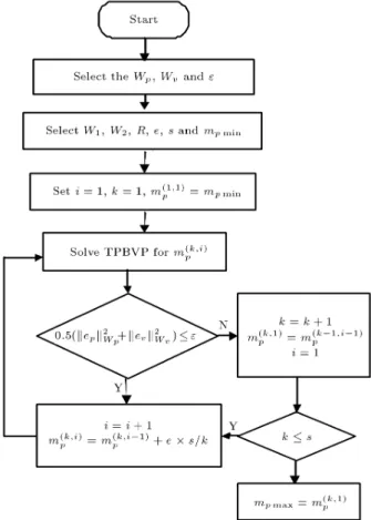
In this section, the manner of calculating the maximum payload and its corresponding optimal trajectory at a point-to-point motion for the robot manipulators is presented. The maximum payload algorithm has been shown in Figure 1. e is the accuracy at the maximum payload calculation and s is the iterations number. With the aid of this algorithm, the maximum payload for the supposed penalty matrices can be found. The solution method is based on increasing the payload from its minimum value, mp min, until the maximum
payload value can be found. The presented solution algorithm has two loops. The loop index, (i), increases the payload at each iteration while the other one, (k),
adjusts the jump interval. Therefore, the accuracy in payload calculation is guaranteed, as well as the approaching rate to the nal answer.
A TPBVP solution for mp mp max desired
accuracy in the TPBVP solution is achievable, thus, Equation 26 is satised. While, for mp > mp max, the
obtained error becomes considerably larger than ". For mp max, the nal error will be less than " and motors
work on their maximum capacity. Under this condition, carrying the payload more than mp max is required,
in order to apply torque to more than their limit, but, this is impossible, because the torque constraints are satised at each iteration in the TPBVP solution. Consequently, the error value becomes signicantly large. Using this fact, a criterion for maximum payload calculation is employed in the presented algorithm.
SIMULATION
In this section, simulations are performed for a two-link and a three-link manipulator. Simulation for the two-link manipulator is carried out for two cases. In the rst case, the maximum payload and its corresponding optimal trajectory is determined for dened penalty matrices. The second case is determination of the maximum payloads for the dierent values of penalty matrices and obtaining a set of optimal paths. Simula-tion for the three-link manipulator is performed for an articulated robot used in [3], and the obtained results are compared with existing results. By comparison of the simulation results, the eciency of the proposed method will be investigated and the superiority of this method over the ILP method will be illustrated.
Simulation for a Two-Link Manipulator
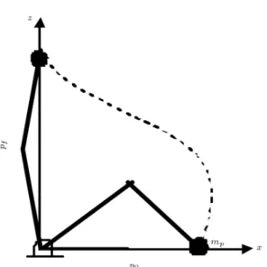
A two link-manipulator at a vertical plan is considered as shown in Figure 2.
All required parameters of the robot manipulator are given in Table 1.
The initial position of the end-eector in the XZ plan at t = 0 is p0 = (1; 0) and the nal position at
t = 1 s is pf = (0; 1:73). The initial and nal velocity
is zero. Using Equation 2, the state vectors can be dened as follows:
Table 1. Simulation parameters. Parameter Value Unit Length of links L1= L2= 1 M
Mass m1= 2, m2= 2 kg
Moment of inertia I1= I2= 0:166 kg.m2
Max. no load speed !s1= !s2= 5:6 Rad/s
Actuator stall torque s1= s2= 104 N.m
Figure 2. Schematic of robot and the optimal path.
X1=
q1(t)
q2(t)
=
x1(t)
x3(t)
;
X2=
_q1(t)
_q2(t)
=
x2(t)
x4(t)
;
U =
u1(t)
u2(t)
; (27)
where q1 and q2 are angular positions, _q1 and _q2 are
angular velocity of rst and second link and u1 and
u2 are the rst and second motor torques. From the
inverse kinematic equations, the boundary condition can be expressed as:
x10= 60; x30= 120;
x1f= 120; x3f= 60;
x20= 0; x40= 0; x2f = 0; x4f = 0: (28)
Using Equation 19, the state-space form of the dynamic equations is changed to be:
_
X1= X2; X_2= N(X1; X2) + Z(X1)U: (29)
The objective function is expressed in the following form:
L(X; U; mp)=12X1TW1X1+21X2TW2X2+12UTRU;
(30) and the co-state functions are considered as:
1=
x5(t)
x7(t)
; 2=
x6(t)
x8(t)
Four equations concerned with co-state function are obtained from Equation 20 as follows:
_ 1= W1X1 X@
1[N(X) + ZU] T
2;
_ 2= W2X2 1 X@
2[N(X)] T
2: (32)
The control values from Equations 21 and 23 can be written as:
U = 8 > < > :
U+ R 1Z(X1) 2> U+
R 1Z(X
1) 2 U < R 1Z(X1) 2<U+
U R 1Z(X1) 2< U (33)
U+and U are substituted from Equation 24 into this
equation, so that the control value, U, is calculated in terms of the states, co-states and penalty matrices values. By substituting Equation 33 into Equations 29 and 32, eight nonlinear ordinary dierential equations will be obtained. For the sake of massive calculation, deriving the equations in details are not presented. Eight equations given in Equations 29 and 32, with eight boundary conditions given in Equation 28, con-struct a TPBVP. This problem can be solved using the BVP4C command in MATLAB r.
Simulation for Maximum Payload Trajectory The accuracy matrices and penalty matrices are con-sidered to be Wp= Wv= diag(1) and W1= W2= [0],
R = diag(1e 5). The desired accuracy in the TPBVP solution and payload calculation is considered as: " = 0:001 and e = 0:01. Using the obtained equations from the previous section and on the basis of the presented algorithm in Figure 1, mp increases from mp min to
mp max. A simulation for the range of mp, given in
Table 2, is performed. The maximum payload for these values of penalty matrices is found to be 5.53 kg.
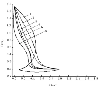
In Figures 3 to 5, 1-6 labels denote six existing cases of Table 2. Figure 3 shows the end-eector trajectories in the XZ plan for dierent values of payload. The sixth trajectory is the optimal path with the maximum payload capacity. The torque curves of the rst and second joints are shown in Figure 4a and 4b, repectively. As shown in these graphs, by increasing the payload, the required torque becomes more and torque curves lay on their own limits, until the payload reaches its maximum value. For the sixth case, the highest possible values of the torque
Table 2. The values of mp used in the simulation.
i 1 2 3 4 5 6
mp max 0.1 2 4 5 5.3 5.53
Figure 3. End-eector trajectories in XZ plan.
Figure 4a. Torques of joints 1.
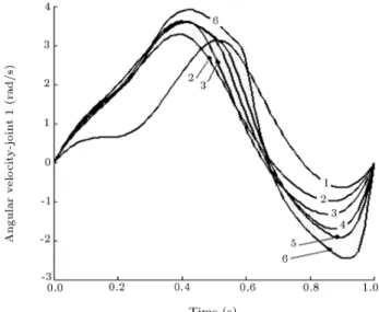
Figure 5a. Angular velocities of joints 1.
Figure 5b. Angular velocities of joints 2.
are applied and an increase in the payload of more than 5.53 kg is required to apply the torque beyond the limits. The angular velocities of the rst and second joints for dierent values of payload are given in Figures 5. It can be seen that increasing the payload leads to more velocity in the joints.
mp max = 5:53 kg is the maximum payload for
the given penalty matrices, while, by considering the other penalty matrices, some new optimal trajectories with dierent specications can be obtained. To illustrate this aspect, some simulations are done for the dierent values of W2 given in Table 3. The
Table 3. The values of mpused to simulation.
i 1 2 3 4
W2 0 0.005 0.05 0.25
mp max(kg) 5.53 5.7 5.96 5.75
other penalty matrices remain the same as the previous values. In this table, the diagonal component of W2
and the calculated maximum payload for each case are indicated.
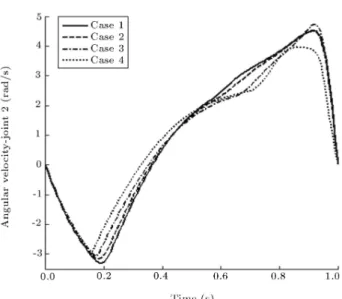
Figure 6 shows the dierent maximum payload trajectories and Figure 7 illustrates the angular ve-locities of the rst and second joints. As expected, by increasing W2, the velocity values decrease and
various optimal paths have been attained. By changing W2 from 0.0 to 0.05, the maximum payload increases
from 5.53 kg to 5.96 and, by further growing in W2,
the maximum payload reduces. The torques and the torque limits for dierent values of mp max are shown
in Figure 8. It can be seen that, in each case, the torque curves have been laid on their limits. All of these trajectories are the maximum payload paths,
Figure 6. Max. payload trajectories.
Figure 7b. Angular velocities of joint 2.
Figure 8a. Torques of joint 1.
Figure 8b. Torques of joint 2.
while they travel dierent paths in work space and have dierent velocities and torque curves.
CONCLUSION
In this paper, a new method, based on the optimal control approach, is proposed to nd the maximum payload trajectory. In this method, the complete form of the obtained nonlinear equation is used and, unlike previous works, linearization of the equations, dierentiation, with respect to payload and joint pa-rameters, or the use of a xed-order polynomial as the solution form, is not required. In the presented method, the problem of determining the maximum payload trajectory converts to the standard form of a two-point boundary value problem, the solution for which has numerous commands, using dierent software, such as MATLAB, C++ or FORTRAN. The BVP4C command in MATLAB was used to solve the problem. Simulations are undertaken for two types of manipulator. For the two-link manipulator, the maxi-mum payload for a given penalty matrix is determined. After that, the dierent maximum payloads for a range of penalty matrices are obtained. It is illustrated that, by changing the penalty matrices values, various optimal trajectories with dierent maximum payloads and path specications are obtained. Therefore, the designer is able to select a suitable path through a set of obtained paths.
In [3], the maximum payload of a three-link manipulator is calculated using iterative linear pro-gramming. In order to verify the proposed method, simulation is performed for this case study and reason-able agreement is observed between the two dierent methods. It is found that the obtained results from the proposed method have some superiority over the ILP method used, generally, in previous works. The ILP method leads to a single solution, whereas the optimal control method attains various optimal trajectories. So, the ILP answer is one of the optimal control results. The ILP method has a convergence problem, wherein the initial path must be very close to the optimal path, while, in the proposed method, an initial guess is not required.
REFERENCES
1. Wang, L.T. and Ravani, B. \Dynamic load carrying capacity of mechanical manipulators-Part 1", J. of Dynamic Sys., Measurement and Control, 110(1), pp. 46-52 (1988).
2. Yao, Y.L., Korayem, M.H. and Basu, A. \Maximum allowable load of exible manipulators for given dy-namic trajectory", Robotics and Computer Integrated Manufacturing, 10(4), pp. 301-308 (1994).
capacity of mechanical manipulators-Part 2", J. of Dynamic Sys., Measurement and Control, 110(1), pp. 53-61 (1988).
4. Korayem, M.H. and Ghariblu, H. \Maximum allowable load of mobile manipulator for two given end points of end-eector", Int. J. of Adv. Manuf. Technol., 24(10), pp. 743-751 (2004).
5. Korayem, M.H. and Gariblu, H. \Analysis of wheeled mobile exible manipulator dynamic motions with maximum load carrying capacities", Robotics and Au-tonomous Systems, 48(3), pp. 63-76 (2004).
6. Gariblu, H. and Korayem, M.H. \Trajectory optimiza-tion of exible mobile manipulators", Robotica, 24(3), pp. 333-335 (2006).
7. Wang, C-Y.E., Timoszyk, W.K. and Bobrow, J.E. \Payload maximization for open chained manipulator: Finding motions for a Puma 762 robot", IEEE Trans-actions on Robotics and Automation, 17(2), pp. 218-224 (2001).
8. Koivo, A.J. and Arnautovic, S.H. \Dynamic optimum control of redundant manipulators", Proc. IEEE Int. Conf. on Robotics and Automation, pp. 466-471 (1991).
9. Mohri, A., Furuno, S., Iwamura, M. and Yamamoto, M. \Sub-optimal trajectory planning of mobile ma-nipulator", Proc. IEEE Int. Conf. on Robotics and Automation, pp. 1271-1276 (2001).
10. Kelly, A. and Nagy, B. \Reactive nonholonomic tra-jectory generation via parametric optimal control", International Journal of Robotics Research, 22(8), pp. 583-601 (2003).
11. Furuno, S., Yamamoto, M. and Mohri, A. \Trajectory planning of mobile manipulator with stability con-siderations", Proc. IEEE Int. Conf. on Robotics and Automation, Taiwan, pp. 3403-3408 (2003).
12. Wilson, D.G., Robinett, R.D. and Eisler, G.R. \Dis-crete dynamic programming for optimized path plan-ning of exible robots", Proc. IEEE Int. Conf. on lntelligent Robots and Systems, Japan (2004).
13. Hull, D.G. \Conversion of optimal control problems into parameter optimization problems", J. of Guid-ance, Control and Dynamics, 20(1), pp. 57-60 (1997). 14. Kirk, D.E., Optimal Control Theory; an Introduction,