Convergence Analysis of Spline Solution of Certain Two-Point Boundary Value Problems

(1)

Vol. 16, No. 2, pp. 128{136 c

Sharif University of Technology, December 2009 Research Note

Convergence Analysis of Spline Solution of

Certain Two-Point Boundary Value Problems

J. Rashidinia

1;

_{, R. Jalilian}

2

_{and R. Mohammadi}

1

Abstract. The smooth approximate solution of second order boundary value problems are developed by using non-polynomial quintic spline function. We obtained the classes of numerical methods, which are second, fourth and six-order. For a specic choice of the parameters involved in a non-polynomial spline, truncation errors are given. A new approach convergence analysis of the presented methods are discussed. Three test examples are considered in our references. By considering the maximum absolute errors in the solution at grid points and tabulated in tables for dierent choices of step size, we conclude that our presented methods produce accurate results in comparison with those obtained by existing methods. Keywords: Two-point boundary value problem; Non-polynomial Quintic spline; Convergence analysis.

INTRODUCTION

We consider the two-point boundary value problem: u00_{+ g(x)u = q(x);}

u(a) = ; u(b) = ;

a x b; (1)

where g(x) and q(x) are continuous functions on [a; b] and a, b, and are arbitrary real nite constants. Such problems arise in the theory which describes the deection of plates and a number of other scientic applications. In general, it is dicult to obtain the analytical solution of Equations 1 for arbitrary choices of g(x) and q(x). We usually resort to a numerical method for obtaining an approximate solution of the problem (Equations 1). A more commonly used nite dierence method for solving Equations 1 numerically is discussed by many authors and we refer the reader, 1. School of Mathematics, Iran University of Science and

Tech-nology, Tehran, P.O. Box 1684413114, Iran.

2. Department of Mathematics, Ilam University, Ilam, P.O. Box 69315-516, Iran.

*. Corresponding author. E-mail: [email protected] Received 30 April 2008; received in revised form 21 January 2009; accepted 16 March 2009

in particular, to Fox [l], Henrici [2], Aziz et al. [3], Bramble et al. [4], Fischer et al. [5] and Usmani [6]. The possibility of using spline functions for obtaining a smooth approximate solution of Equations 1 is briey discussed by Ahlberg et al. [7]. Since then, Albasiny and Hoskins [8], Bickley [9], Fyfe [10] and Sakai and Usmani [11] have used the cubic spline for obtaining approximations. Bhatta et al. [12] have used the spline functions of degrees seven and eight and Usmani and Wasrt [13] used the Quintic spline. Also, Usmani and Sakai [14] used a cubic and a quartic spline. Khan [15] used a parametric cubic spline function to develop a numerical method for computing smooth approximations to the solution for second order boundary value problems. Recently, Ramadan et al. [16] developed a sixth-order method based on a quintic non-polynomial spline function for the solution of high order two point boundary value problems, but in application, they solved only second and fourth order boundary value problems. Their method suers from boundary conditions and due to this, the order of accuracy of their method is reduced. Besides, in the convergence analysis, they assumed more restrictions on Equations 1 and an arising coecient matrix.

In this paper, we have derived a uniformly conver-gent mesh dierence scheme using a non-polynomial spline for the solution of Equations 1. Analysis of the methods shows a second, fourth and

(2)

sixth-order convergent for arbitrary , , p, r and s. In this article, rst, the consistency relation of our non-polynomial quintic spline in [17] is used for the solution of Equations 1. Then, the methods and the development of boundary conditions are described and classes of the methods are discussed. Following that a new approach for convergence analysis is presented. Here, we obtained the restriction on function g only. Finally, some numerical evidence is included to show the practical applicability and superiority of our meth-ods.

DESCRIPTION OF THE METHODS AND DEVELOPMENT OF BOUNDARY

CONDITIONS

Let us consider a mesh with nodal points xi on [a; b],

such that:

: a = x0< x1< x2< < xn 1< xn= b;

where h = b a

n for i = 1(1)n. We also denote the

function value u(xi) by ui.

For each segment [xi; xi+1]; i = 0; 1; 2; ; n 1,

by using the non-polynomial quintic spline relation derived in our paper [17], we have:

pMi 2+ rMi 1+ sMi+ rMi+1+ pMi+2

= 1

h2[(ui+2+ ui 2)

+ 2( )(ui+1+ ui 1) + (2 4)ui]; (2)

where:

p = 1+₆;

r = 2

1

6(2 + ) (1 1

;

s = 2

1

6( + 4) + (1 21

;

=

1 2

( csc 1);

=

1 2

(1 cot );

1= 1₂

1

6

;

1= 1₂

1

3

:

At mesh point xi, the proposed dierential Equations 1

may be discretized by:

Mi+ giui = qi; (3)

where:

Mi = S00i(xi);

gi= g(xi);

qi= q(xi);

and:

ui= u(xi):

Substituting Equation 3 in spline Relation 2, we obtain: ( + ph2_g

i 2)ui 2+ (2( ) + h2rgi 1)ui 1

+(2 4+sh2_g

i)ui+(2( )+h2rgi+1)ui+1

+(+ph2_g

i+2)ui+2=h2(p(qi 2)+r(qi 1) + s(qi)

+ r(qi+1) + p(qi+2)); (4)

i = 2(1)n 2:

To obtain a unique solution for this system (Equa-tion 4), we need two more equa(Equa-tions to be associated, so we use the following boundary conditions:

(a) Following [17], the second-order boundary formula is:

u1 2u2+ u3= h 2

6 (u001+ 4u002+ u003);

i = 1;

un 3 2un 2+ un 1

=h₆2(u00

n 3+ 4u00n 2+ u00n 1);

i = n 1; (5)

using Equation 3, we have: (1 + h₆2g1)u1+ ( 2 +4h 2

6 g2)u2

+ (1 +h₆2g3)u3= h 2

6 [q1+ 4q2+ q3]; (1 + h₆2gn 3)un 3+ ( 2 +4h

2

6 gn 2)un 2

+ (1 +h₆2gn 1)un 1

(3)

(b) Following [17], the fourth-order boundary formula is:

u1 2u2+u3=h 2

12(u001+10u002+u003);

i = 1;

un 3 2un 2+ un 1= h 2

12(u00n 3+ 10u00n 2

+ u00 n 1);

i = n 1; (6)

using Equation 3, we have:

(1 +h₁₂2g1)u1+ ( 2 +10h 2

12 g2)u2

+ (1 +h₁₂2g3)u3= h 2

12[q1+ 10q2+ q3];

(1 +h₁₂2gn 3)un 3+ ( 2 +10h 2

12 gn 2)un 2

+ (1 +h2

12gn 1)un 1

=h₁₂2[qn 3+ 10(qn 2) + qn 1];

(c) In order to obtain the sixth-order boundary for-mula, we dene the following identities:

3

X

k=0

akuk+ h2 5

X

k=0

bku00k+ t1h8u(8)0 ;

i = 1;

3

X

k=0

akun k+ h2 5

X

k=0

bku00n k+ tn 1h8u(8)n ;

i = n 1; (7)

in order to obtain unknown coecients a and b in Relations 7, by Taylor's expansion, we obtain:

(a0; a1; a2; a3) = ( 10; 19; 8; 1);

t1= tn 1= (₆₀₄₈₀2179 );

(b0; b1; b2; b3; b4; b5)

=

179 240;

1057 120 ;

39 40;

41 60;

61 240;

1 24

:

CLASSES OF THE METHODS

By expanding Equation 4 in the Taylor's series about xi, we obtain the following local truncation error:

ti=

1

6(7 + ) (4p + r)

h4_u(4) i

+

1

180(31 + ) 1

12(16p + r)

h6_u(6) i ;

+

1

131040(1611 + 31) 1

360(4p + r)

h8_u(8) i

+ O(h9_); _{2 i n 2:} ₍₈₎

By using the above truncation error to eliminate the coecients of various powers, h, we can obtain classes of the methods. For any choice of , , p, r and s, whose + = 1

2 and with boundary formulas

(Relations 5 to 7) we obtain the following methods.

Second-Order Method For:

(; ) =

1 4;

1 4

;

and:

p = 0:040634839941134321703; r = 0:25412730690212937985; s = 0:41047570631347259688;

we obtain the second-order method, ti= O(h4).

Fourth-Order Method For:

(; ) = (1₆;1₃); and:

p = ₁₂₀1 ;

r = ₁₂₀26 ;

s = 66 120;

(4)

Sixth-Order Method For

(; ) = (₁₂1 ;₁₂5 ); and:

p = ₃₆₀1 ;

r = ₃₆₀56;

s = 246₃₆₀;

we obtain the sixth-order method, ti= O(h8).

CONVERGENCE ANALYSIS

In this section, we investigate the new approach con-vergence analysis of the sixth-order associated method, a boundary formulas (Relations 7). The given system can be considered in matrix form as:

(i) AU = C + T; (ii) AU = C;

(iii) AE = T; (9)

where:

U = (ui); U = (ui); C = (ci);

T = (ti); E = (ei);

are (n 1)-dimensional column vectors. Matrix A is dened by:

A = (A0A1+ 6A0) + B;

where A is a monotone ve band matrix of order n 1, and A0= (aij) is a tri-diagonal matrix dened by:

aij=

8 > < > :

2; i = j = 1; 2; ; n 1; 1; ji jj = 1;

0; otherwise;

(10)

and A1= (aij), is a tri-diagonal matrix dened by:

a ij= 8 > < > :

4; i = j = 1; 2; ; n 1; 1; ji jj = 1;

0; otherwise;

(11)

B = h2_{QG with G = diag(g}

i), i = 1; 2; ; n 1, and:

(A0A1+ 6A0) =

2 6 6 6 6 6 6 6 6 6 6 6 6 6 6 6 4

19 8 1

8 18 8 1

1 8 18 8 1

... ... ... ... ... ... ... ... ... ...

... ... ... ... ...

1 8 18 8 1

1 8 18 8

1 8 19

3 7 7 7 7 7 7 7 7 7 7 7 7 7 7 7 5 ; (12) Q = 2 6 6 6 6 6 6 6 6 6 6 6 6 6 6 6 6 6 6 6 6 6 6 6 6 6 6 6 6 6 6 6 4 1057

120 3940 4160 24061 672

360 2952360 672360 36012 12

360 672360 2952360 672360

... ... ... ... ... ... 1 24 12 360 ... ... ... ... ... ... ... ... ... 12

360 672360 2952360 672360 36012 12

360 672360 2952360 672360 1

24 24061 4160 3940 1057120

3 7 7 7 7 7 7 7 7 7 7 7 7 7 7 7 7 7 7 7 7 7 7 7 7 7 7 7 7 7 7 7 5 : (13)

(5)

Vector C is given by: ci = 8 > > > > > > > > > > > > > > > > > > > > > > > > > > > > > > > > > > > > > > > > > > > > > > > > > > > > > > > > > > > > > > > > > > > > > > < > > > > > > > > > > > > > > > > > > > > > > > > > > > > > > > > > > > > > > > > > > > > > > > > > > > > > > > > > > > > > > > > > > > > > > :

10 h2

" 179

240(q0 g0) + 1057

120 q1+ 39 40q2

+41 60q3

61 240q4+

1 24q5

# ;

i = 1;

12h₃₆₀2[(q0 g0)+56q1+246q2+56q3+q4];

i = 2;

12h2

360 [qi 2+ 56qi 1+ 246qi+ 56qi+1+ qi+2];

i = 3; ; n 3;

12h₃₆₀2[(qn gn) + 56qn 1+ 246qn 2

+ 56qn 3+ qn 4];

i = n 2;

10 h2_[179

240(qn gn) + 1057

120 qn 1 +39

40qn 2+ 41 60qn 3

61 240qn 4 + 1

24qn 5]; i = n 1:

(14)

Vector T is the local truncation error vector and is dened as:

ti=

8 > > > > > > > > < > > > > > > > > : 2179

60480h8u(8)(1)+O(h9); a < 1< x5

i = 1;

173

262080h8u(8)(i)+O(h9); xi 2<i<xi+2

i=2; ; n 2;

2179

60480h8u(8)(n 1)+O(h9); xn 5<n 1<b

i=n 1:

(15)

Lemma 1

If M is a square matrix of order n and kMk < 1, then (I + M) 1_{exists and k(I + M)} 1_{k <} 1

(1 kMk).

To explain the existence of A 1_{, since A =}

(A0A1+ 6A0) + B, we have to show (A0A1+ 6A0)

is nonsingular. By using Lemma 1 and Henrici [2], we shall rst require bounds for the element of (A0) 1.

If A 1

0 = (aij), then:

a ij= 8 > < > : j(n i)

n ; i j; i(n j)

n ; i j;

(16)

and we get:

n X j=1 a ij= i X j=1 j(n i) n + n X j=i+1 i(n j) n (n)2

8 ; (17)

where the equality holds only if n is odd. Inequality can be written as:

kA₀1k (b a)_8h₂ 2: (18)

Also, by using [13] we have:

kA 1 1 k 1₂;

(A0A1+ 6A0) 1= (I +₆1A1) 1(6A0) 1: (19)

By using Lemma 1 (I + 1

6A1) 1 exists and we get

bounds for k(A0A1+ 6A0) 1k,

k(A0A1+ 6A0) 1k k(6A0) 1_k

1 k1 6A1k

=(b a)_44h₂2; (20)

where k:k represents the 1-norm in the matrix vector.

Lemma 2

Matrix A = (A0A1+ 6A0) + B is nonsingular, if:

kgk < _{3(b a)}11 ₂;

(6)

Proof Since

A 1_{= [(A}

0A1+ 6A0) + B] 1

= [I + (A0A1+ 6A0) 1B] 1(A0A1+ 6A0) 1;

it is sucient to show that [I + (A0A1+ 6A0) 1B] is

nonsingular. Moreover, we know that in the case of a sixth-order method we can obtain:

kQk 12:

Also, using Lemma 1, if k(A0A1+ 6A0) 1Bk < 1, then

(I + (A0A1+ 6A0) 1B) 1 exists. Also, we get:

k(I + (A0A1+ 6A0) 1B) 1k

< _{1 k(A} 1

0A1+ 6A0) 1Bk;

where:

k(A0A1+ 6A0) 1Bk k(A0A1+ 6A0) 1kkBk

(b a)2

44h2 (h2kQkkgk) < 1;

and then, we have: kgk < 11

3(b a)2:

Theorem 1

Let u(x) be the exact solution of the boundary value problem (Equations 1) and assume that ui, i =

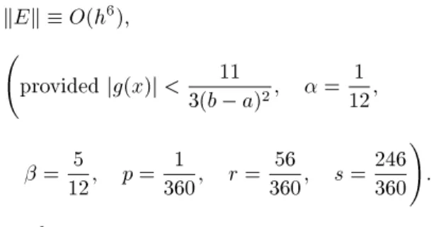
1; 2; ; n 1 be the numerical solution obtained by solving the system (Equation 9 (iii)), then we have:

kEk O(h6_);

provided jg(x)j < _{3(b a)}11 ₂; = ₁₂1 ;

= ₁₂5 ; p =₃₆₀1 ; r =₃₆₀56; s = 246₃₆₀ !

:

Proof

The main purpose is to drive a band on kEk. Using Equation 9 (ii) and Lemma 2, we have:

E = A 1_T

= [I + (A0A1+ 6A0) 1B] 1(A0A1+ 6A0) 1T;

kEk k[I + (A0A1+ 6A0) 1B] 1k

k(A0A1+ 6A0) 1kkT k: (21)

By using Lemma 1, we get:

kEk _{1 k[(A}k(A0A1+ 6A0) 1kkT k

0A1+ 6A0) 1B]k; (22)

provided k[(A0A1+ 6A0) 1B]k < 1, also we have:

kT k 2179h8M8

60480 ; (23)

where M8= maxabju(8)()j.

Using Equations 20, 22, 23 and Lemma 2, we obtain:

kEk _{60480(44 12(b a)}2179(b a)2h6M₂8_kgk) O(h6_); ₍₂₄₎

provided that:

kgk < _{3(b a)}11 ₂: (25)

NUMERICAL ILLUSTRATIONS

In order to test the viability of the proposed methods, based on a non-polynomial spline, and to demonstrate its convergence computationally, we consider the fol-lowing four test boundary value problems.

Example 1

We consider the following boundary-value problem:

u00_{= u + x}2 _2; _{u(0) = 0; u(1) = 1;}

with the exact solution, u(x) = 2sinh(x)_sinh(1) x2_.

This problem has been solved using our methods with dierent values of n = 8; 16; 32; 64 and the maximum absolute errors in solutions are tabulated in Table 1.

Table 1. Observed maximum absolute errors for Example 1.

n

Second-Order

= 1

4; = 14

Fourth-Order

= 1

6; = 13

Sixth-Order

= 1

12; = 125

8 1:09 10 4 _{5:22 10} 8 _{8:75 10} 11

16 3:06 10 5 _{2:31 10} 9 _{5:74 10} 13

32 8:11 10 6 _{1:34 10} 10 _{2:30 10} 14

(7)

Table 2. Observed maximum absolute errors for Example 2. n

Second-Order

= 1

4, = 14

Fourth-Order

= 1

6, = 13 Fourth-Order [13]

8 2:42 10 3 _{2:64 10} 6 _{1:10 10} 6

16 6:80 10 4 _{1:26 10} 7 _{1:09 10} 7

32 1:80 10 4 _{7:41 10} 9 _{7:51 10} 9

64 4:65 10 5 _{4:65 10} 10 _{4:81 10} 10

128 1:18 10 5 _{2:95 10} 11 _{3:03 10} 11

256 2:98 10 6 _{1:78 10} 12 _{1:85 10} 12

512 7:47 10 7 _{4:35 10} 13 _{6:48 10} 13

1024 1.8710 7 _4.6010 13 _{7:64 10} 13

n

Sixth-Order

= 1

12, = 125 Seventh-Order [12]

8 8:02 10 9 _{1:44 10} 7

16 5:01 10 11 _{1:41 10} 9

32 1:16 10 12 _{1:23 10} 11

64 2:55 10 15 _{1:01 10} 13

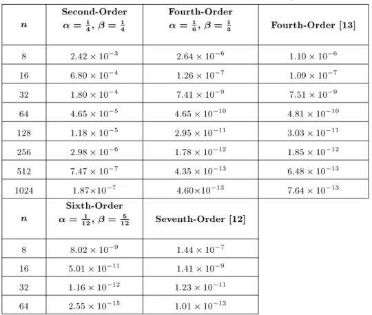
Example 2

We consider the following boundary-value problem: u00_{= u 4xe}x_; _{u(0) = u(1) = 0;}

with the exact solution, u(x) = x(1 x)ex_.

We applied our methods to solve this problem with n = 8; 16; 32; 64; 128; 256; 512; 1024 and the com-puted solutions are compared with the exact solution at grid points. The maximum absolute errors at the nodal points, maxju(xi) uij, are given to compare

with [12,13]. The observed maximum absolute errors are tabulated in Table 2.

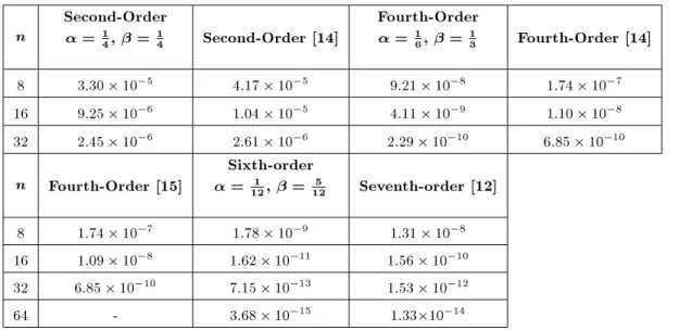
Example 3

We consider the following example in [12,14,15]: x2_u00_{= 2u x;} _{u(2) = u(3) = 0;}

with the exact solution, u(x) = (19x 5x2 36x)

38 .

We applied our methods to solve this problem for n = 8; 16; 32; 64 and the computed solutions are compared with the exact solution at grid points. The observed maximum absolute errors are tabulated in Table 3. In this table we compared our results with the results given in [12,14,15]. This shows that our results are more accurate.

Example 4

We consider the following example in [16]:

u00_{= u + (4 2x}2_{) sin x + 4x cos x;}

u(0) = u(1) = 0;

with the exact solution, u(x) = (x2 _{1) sin x.}

We applied our sixth-order method to solve this problem for n = 8; 16; 32 and 64. The computed solutions are compared with the exact solution at grid points. The observed maximum absolute errors are tabulated in Table 4. In this table, we compared our results with the results obtained by the methods in [16] and also with the results obtained by [18,19] which are reported in [16]. This shows that our results are more accurate.

CONCLUSION

The approximate solutions of second-order linear boundary-value problems using a non-polynomial spline, show that our methods are better in the sense of accuracy and applicability. These have been veried by the maximum absolute errors, max jeij, given in the

(8)

Table 3. Observed maximum absolute errors for Example 3. n

Second-Order

= 1

4, = 14 Second-Order [14]

Fourth-Order

= 1

6, = 13 Fourth-Order [14]

8 3:30 10 5 _{4:17 10} 5 _{9:21 10} 8 _{1:74 10} 7

16 9:25 10 6 _{1:04 10} 5 _{4:11 10} 9 _{1:10 10} 8

32 2:45 10 6 _{2:61 10} 6 _{2:29 10} 10 _{6:85 10} 10

n Fourth-Order [15]

Sixth-order

= 1

12, = 125 Seventh-order [12]

8 1:74 10 7 _{1:78 10} 9 _{1:31 10} 8

16 1:09 10 8 _{1:62 10} 11 _{1:56 10} 10

32 6:85 10 10 _{7:15 10} 13 _{1:53 10} 12

64 - 3:68 10 15 _1.3310 14

Table 4. Observed maximum absolute errors for Example 4. n Sixth-Order Ramadan [16] Islam [18] Al-Said [19]

8 7:35 10 9 _{7:24 10} 9 _{2:37 10} 5 _{6:49 10} 4

16 1:68 10 11 _{1:16 10} 10 _{1:60 10} 6 _{1:70 10} 4

32 5:06 10 13 _{1:82 10} 12 _{1:03 10} 7 _{4:15 10} 5

64 4:12 10 15 _{6:51 10} 14 _{6:60 10} 9 _{1:82 10} 5

REFERENCES

1. Fox, L., The Numerical Solution of Two Point Bound-ary Value Problems in OrdinBound-ary Dierential Equa-tions, Oxford University Press, London (1957). 2. Henrici, P., Discrete Variable Methods in Ordinary

Dierential Equations, Wiley, New York (1961). 3. Aziz, A.K. and Hubbard, B.E. \Bounds for the

solu-tion of the Sturm-Liouville problem with applicasolu-tions to nite dierence methods", SIAM. J., 12, pp. 163-168 (1964).

4. Bramble, J.H. and Hubbard, B.E. \On a nite dier-ence analogue of an elliptic boundary problem which is neither diagonally dominant nor of nonnegative type", J. Math. Phys., 43, pp. 117-132 (1964).

5. Fischer, C.F. and Usmani, R.A. \Properties of some tri-diagonal matrices and their applications to bound-ary value problems", SIAM. J. Num. Anal., 6, pp. 127-132 (1969).

6. Usmani, R.A. \A method of high order accuracy for the numerical integration of boundary value problems", BIT, 13, pp. 458-469 (1973).

7. Ahlberg, J.H., Nilson, E.N. and Walsh, J.L., The Theory of Splines and Their Applications, Academic Press, New York (1967).

8. Albasiny, E.L. and Hoskins, W.D. \Cubic spline solu-tion of two point boundary value problem", Comput. J., 12, pp. 151-153 (1969).

9. Bickley, W.G. \Piecewise cubic interpolation and two-point boundary-value problems", Comput. J., 11, pp. 206-208 (1968).

10. Fyfe, D.J. \The use of cubic splines in the solution of two-point boundary-value problems", Comput. J., 12, pp. 188-192 (1969).

11. Sakai, M. and Usmani, R.A. \Quadratic spline and two point boundary value problems", Publ. RIMS, Kyoto Univ., 19, pp. 7-13 (1983).

12. Bhatta, S.K. and Sastri, K.S. \A seventh order global spline procedure for a class of boundary value prob-lems", Int. J. Computer Math., 41(3), pp. 99-114 (1991).

13. Usmani, R.A. and Wasrt, S.A. \Quintic spline solu-tions of boundary value problems", Comput. Math. with Appl., 6, pp. 197-203 (1980).

14. Usmani, R.A. and Sakai, M. \A connection between quartic spline and Numerov solution of a boundary value problem", Int. J. Comput. Math., 26, pp. 263-273 (1989).

15. Khan, A. \Parametric cubic spline solution of two point boundary value problems", Appl. Math. Com-put., 154, pp. 175-182 (2004).

16. Ramadan, M.A., Lashien, I.F. and Zahra, W.K. \High order accuracy non-polynomial spline solutions for 2th order two point boundary value problems", Appl. Math. Comput., 204, pp. 920-927 (2008).

(9)

17. Rashidinia, J., Jalilian, R. and Mohammadi, R. \Non-polynomial spline methods for the solution of a system of obstacle problems", Appl. Math. Comput., 188, pp. 1984-1990 (2007).

18. Islam, S.U., Noor, M.A., Tirmizi, I.A. and Khan, M.A. \Quadratic non-polynomial spline approach to the solution of a system of second-order

boundary-value problems", Appl. Math. Comput., 179, pp. 153-160 (2006).

19. Al-Said, E.A. \The use of cubic splines in the numeri-cal solution of a system of second-order boundary-value problems", Computers Math. Applic., 42, pp. 861-869 (2001).