Sharif University of Technology
Scientia IranicaTransactions E: Industrial Engineering www.scientiairanica.com
Research Note
Sample size determination for C
p
comparisons
S.M. Chen
a, J.T. Liaw
aand Y.S. Hsu
b;a. Department of Mathematics, Fu-Jen Catholic University, New Taipei City, 24205, Taiwan, R.O.C. b. Department of Mathematics, National Central University, Taoyuan City, Chung-Li, 32054, Taiwan, R.O.C. Received 31 January 2015; received in revised form 6 July 2015; accepted 19 October 2015
KEYWORDS Process capability index;
Maximum likelihood estimator;
Biased estimator; Unbiased estimator; Cp;
Cpk.
Abstract. Comparison of quality for products (supplies and goods) is extremely important for manufacturers and consumers. Based on correct comparisons, manufacturers and consumers can nd better suppliers to cooperate and better merchandise to purchase, respectively. Quality is often measured and compared by process capability indices, among which Cp is very eective, simple to apply, and particularly useful for the rst round of
comparison. In practice, Cp is unknown and should be estimated from observations. Let
d
Cpidenote the maximum likelihood estimator obtained from normal process, Xi, with index
value Cpi; i = 1; 2. If dCp1> (<)dCp2 is observed, we will conclude that Cp1> (<)Cp2 and
decide that X1is better (worse) than X2. Given a small and positive number, , there is no
need to make comparison when (1 )Cp2< Cp1< (1+)Cp2since Cp1is close to Cp2. It is
desirable to observe dCp1> dCp2 with high probability when (1 + )Cp2< Cp1and with low
probability when (1 )Cp2> Cp1. Given 0 < 1, 2 < 1, based on the table constructed
from P (dCp1> dCp2), we demonstrate how to nd the smallest sample size needed to ensure
observing dCp1 > dCp2 with probability greater than 1 1 when (1 + )Cp2 < Cp1 and
smaller than 2 when (1 )Cp2> Cp1.
© 2016 Sharif University of Technology. All rights reserved.
1. Introduction
In order to build up a good credit, producers have to make sure that their products meet customers' requests with high probability. Therefore, process capability analysis is, a necessity. Once a stable process is conrmed in phase I study, process capability analysis can then be designed to estimate the proportion of parts that meets engineering requirements in a stable production process. There are several ways for the purpose; a well-known summary quantitative measure is the process capability index. It is designed for in-dustrial eld for the purpose of process assessment and *. Corresponding author. Tel.: 011-886-3-422-7151 ext 65132;
Fax: 011-886-3-425-7379
E-mail addresses: [email protected] (S.M. Chen); [email protected] (J.T. Liaw); [email protected] and [email protected] (Y.S. Hsu)
improvement for suppliers and consumers; however, it is also used extensively in many dierent elds which include education [1] and medical science [2].
In the past decades, there have been varieties of innovative process capability indices. All of these indices were designed to evaluate the potential ability of processes to meet dierent kinds of requirements. But, as pointed out in [3], none of the new indices has surpassed Cp and Cpkin popularity or ease of use.
Kane [4] introduced index Cp for the very rst
time dened as the fraction between the allowable range of measurements over which the process measure-ment can vary and the range of measuremeasure-ments in which the process is actually varying. It can be expressed as Cp = USL LSL6 , where USL and LSL are the upper
and the lower specication limits, respectively, and is the process standard deviation. The index was named dierently by dierent authors. For example, Finley [5] used the term \capability potential index"
to which Montgomery [6] referred as process capability ratio. Notice that Cp concerns only the spread of a
process not the process mean at all. So, it provides valuable information only when the mean is on tar-get. The index Cp is particularly suitable when the
independent data are from a normal distribution and it is meaningless to use it if the process is not under statistical control.
The index Cp has been proved to be useful
in automotive and manufacturing industries, among others. For instance, it has been applied to piston-rings for an automotive engine [6] and bolts used in bridge construction [7]. Applications to fan housing weight, roller width, exhaust valves, and acrylic coating can be found in [8]. Recent applications of Cp include engine
axle manufacturing process [9], yogurt production [10], and calibration [11,12], etc.
In practice, Cp is rarely known and has to be
estimated from sample. Most of the statistical re-search concerning Cp focus on the standard inferences
including point and interval estimations and test. For examples, the maximum likelihood estimator of Cpwas
proposed by Kane [4], its moments were discussed in Kotz and Johnson [7], and its sampling distribution was investigated by Chan et al. [13], Chou and Owen [14], Chou et al. [15], and Li et al. [16]. It was further shown that the maximum likelihood estimator is biased, but it is asymptotically unbiased when the sample size is large enough (see [3,7,8,17] and references therein for more details). In this paper, we present a dierent and useful study for Cp comparison to be described
explicitly below.
It is not uncommon that dierent manufactories may have dierent qualities for the same product. It is important to recognize the better process, since the better process can serve the consumers better and the worse process can be investigated by the manufacturers for improvements.
Let N(1; 12) and N(2; 22) denote the
dis-tributions of measurements from two manufacturing processes X1 and X2 with potential capability indices
Cp1 = USL LSL61 and Cp2 = USL LSL62 , respectively.
Note that we assume both process have the same upper and lower specication limits. Since it is desirable to have a Cp as large as possible, process X1is considered
to be better (worse) than process X2if Cp1> (<)Cp2.
Unfortunately, Cp1 and Cp2 are often unknown,
and hence cannot be applied to make comparisons. In practice, Cp1 and Cp2 can be inferred from
sam-ples. Let X11; ; X1n and X21; ; X2n denote two
independent samples from N(1; 21) and N(2; 22),
respectively. Let S2 1 = 1n
Pn
i=1(X1i X1)2 and S22 = 1
n
Pn
i=1(X2i X2)2denote the sample variances, where
X1 = n1Pni=1X1i and X2 = n1Pni=1X2i are the
sample means. Since X1; S12; X2, and S22are maximum
likelihood estimators of 1, 12, 2, and 22, respectively,
d
Cp1 = USL LSL6S1 and dCp2 =
USL LSL
6S2 are maximum likelihood estimators of Cp1 = USL LSL61 and Cp2 =
USL LSL
62 , respectively. See Hogg and Craig [18] for more details.
The purpose of this paper is to provide an ecient way to nd the smallest sample sizes that can help choosing the better process between X1 and X2 based
on dCp1 and dCp2. No such study can be found in the
literatures, to the best of our knowledge.
Without loss of generality, assume that dCp1> dCp2
is observed; naturally we decide that Cp1 > Cp2. We
will judge this decision under three cases: Cp1 2 M,
Cp1 2 R, and Cp1 2 L, where L = (0; (1 )Cp2],
M = ((1 )Cp2; (1 + )Cp2), R = [(1 + )Cp2; 1), and
is a small positive number.
We treat M as an indierent zone, since Cp1 is
close to Cp2 when Cp1 2 M, and there is no need to
make comparisons between X1 and X2. In this case,
any decision will be good.
If Cp12 R, then Cp1> Cp2 and our decision will
be good if we observe dCp1> dCp2 with high probability.
In other words, it is desirable to have large value of: min
Cp12RP
d Cp1> dCp2
: (1)
If Cp1 2 L, then Cp1 < Cp2 and our decision will be
good if we observe dCp1 > dCp2 with low probability.
Thus, it is desirable to have small value of: max
Cp12LP
d Cp1> dCp2
: (2)
We explain the maximum in Relation (1) and the minimum in Relation (2) as follows. Note that for xed n, P (dCp1 > dCp2) is a function of Cp1 and Cp2 (see
Appendix), denoted as F (Cp1; Cp2) = P (dCp1 > dCp2).
The minimum value of F over f(Cp1; Cp2)jCp1 > (1 +
)Cp2g is denoted by:
min
Cp12RP (dCp1> dCp2):
The maximum value of F over f(Cp1; Cp2)jCp1 < (1
)Cp2g is denoted by:
max
Cp12LP (dCp1> dCp2):
Given two small positive numbers 1 and 2, we
aim to nd the smallest sample size to ensure: min
Cp12RP
d Cp1> dCp2
> 1 1; (3)
and the smallest sample size to achieve: max
Cp12LP
d Cp1> dCp2
< 2: (4)
Section 2, we will give the form of P (dCp1 > dCp2)
and the proof can be found in the Appendix. In Section 3, illustrations of sample size determinations will be given via some examples. Some remarks concerning the statistical inferences are presented in Section 4. Future study is proposed in Section 5. Conclusions are provided in Section 6.
2. Derivation of probabilities
In order to nd the smallest n that achieves Relations (3) and (4), we need to evaluate P (dCp1 > dCp2). The
proofs of the following results are given in Appendix: PCdp1> dCp2
= (n 1)
2n 2 n 1 2
2
Z
2
(sin t)n 2dt;
(5) where = tan 1(
1=2). When n = 2k + 3; where k
denotes any nonnegative integer, Eq. (5) implies that: PCdp1> dCp2
=22k+1(2k + 2)[ (k + 1)]2 :Xk
i=0
( 1)ik
i
[cos(2)]2i+1+ 1
2i + 1 ; (6)
where cos 2 =22 21
2
1+22. Moreover, when n = 2k + 2: PCdp1> dCp2
= (2k + 1)
22k 2k+1 2
2
(
(sin 2)2k 1(cos 2)
2k +(2k)(2k 2)2k 1 (sin 2)2k 3(cos 2)
+ (2k 1)(2k 3)
(2k)(2k 2)(2k 4)(sin 2)2k 5(cos 2) + +(2k)(2k 2)(2k 4) 2(2k 1)(2k 3) 3 (sin 2)(cos 2) +(2k)(2k 2)(2k 4) 2(2k 1)(2k 3) 3:1 ( 2)
)
; (7)
where:
= tan 1(
1=2); sin 2 = 22 12 1+ 22;
cos 2 = 222 21
1+ 22:
Given n and 2
1 (or
Cp1
Cp2), Eqs. (6) and (7) can be calculated. To save the places, the results for n 2 f3; ; 100g and Cp1
Cp2 2 f0:1; 0:2; ; 0:9; 0:95; 1; 1:05; 1:1; 1:2; ; 2g, are given in Tables 1 to 3.
It is easy to see from Tables 1 to 3 that P (dCp1>
d
Cp2) increases with CCp1p2. Moreover, P (dCp1 > dCp2)
increases (decreases) with n if Cp1
Cp2 > (<)1. It should be noted that the rounding error produces many 0 in Table 1 and many 1 in Table 3. Each 0 represents a positive number less than 0:00001, and each 1 represents a positive number between 1 and 0:99999. 3. Illustrations
In this section, we explain how to use the above results to nd the smallest sample sizes needed to make comparisons so as to achieve the predetermined bounds for probabilities (1) and (2).
Example 1: If = 0:05, then the indierent zone dened in Section 1 is M = [(1 )Cp2; (1 + )Cp2] =
[0:95Cp2; 1:05Cp2], and we treat two processes with
Cp1 and Cp2 equally well when Cp1 2 M. Note that
0.95 and 1.05 are chosen for convenience; they can be replaced by other suitable positive numbers u and v, such that u < 1 and v > 1.
If Cp1 2 R = [1:05Cp2; 1), then Cp1 > Cp2 and
we want P (dCp1 > dCp2) to be large. If Cp1 2 L =
(0; 0:95Cp2], then Cp1 < Cp2 and we want P (dCp1 >
d
Cp2) to be small. For example, if 0.67 and 0.35 are
considered large and small enough, respectively, then the problem becomes what sample size n will ensure that:
min
Cp12RP
d Cp1> dCp2
> 0:67; (8)
and: max
Cp12LP (dCp1> dCp2) < 0:35: (9) Note that 0.67 and 0.35 are chosen for convenience; they can be replaced by any number and , such that 0 < < 1, 0 < < 1, and and are close to 1 and 0, respectively.
In order to achieve Relation (8), we need n 83 by Table 2 (check the rows and columns corresponding to n 83 and Cp1
Cp2 1:05, respectively).
Moreover, Relation (9) is true if n 58 according to Table 2 (check the rows and columns corresponding to n 58 and Cp1
Cp2 0:95, respectively).
Consequently, if n 83, then Relations (8) and (9) will be held simultaneously.
Example 2: If = 0:1, then R = [(1 + )Cp2; 1) =
[1:1Cp2; 1) and L = (0; (1 )Cp2] = (0; 0:9Cp2]. What
sample size n will ensure for Relations (8) and (9)? In order to achieve Relation (8), we need n 23 by Table 2 (check the rows and columns corresponding to n 23 and Cp1
Table 1. PCdp1> dCp2
for given n when Cp1
Cp2 2 f0:1; ; 0:8g.
Cp1
Cp2
n 0.1 0.2 0.3 0.4 0.5 0.6 0.7 0.8
3 0.00990 0.03846 0.08257 0.13793 0.20000 0.26471 0.32886 0.39024 4 0.00167 0.01266 0.03927 0.08327 0.14238 0.21187 0.28643 0.36138 5 0.00029 0.00432 0.01933 0.05183 0.10400 0.17311 0.25331 0.33801 6 0.00005 0.00151 0.00972 0.03287 0.07719 0.14327 0.22618 0.31813 7 0.00001 0.00054 0.00496 0.02111 0.05792 0.11963 0.20329 0.30072 8 0.00000 0.00019 0.00255 0.01369 0.04381 0.10054 0.18362 0.28519 9 0.00000 0.00007 0.00133 0.00894 0.03334 0.08493 0.16649 0.27115 10 0.00000 0.00003 0.00069 0.00587 0.02550 0.07203 0.15142 0.25832 11 0.00000 0.00001 0.00036 0.00387 0.01958 0.06129 0.13806 0.24652 12 0.00000 0.00000 0.00019 0.00256 0.01509 0.05230 0.12615 0.23558 13 0.00000 0.00000 0.00010 0.00170 0.01165 0.04473 0.11548 0.22541 14 0.00000 0.00000 0.00005 0.00113 0.00903 0.03833 0.10587 0.21591 15 0.00000 0.00000 0.00003 0.00076 0.00700 0.03291 0.09720 0.20700 16 0.00000 0.00000 0.00002 0.00051 0.00544 0.02830 0.08934 0.19863 17 0.00000 0.00000 0.00001 0.00034 0.00424 0.02436 0.08221 0.19073 18 0.00000 0.00000 0.00000 0.00023 0.00331 0.02100 0.07572 0.18327 19 0.00000 0.00000 0.00000 0.00015 0.00258 0.01813 0.06981 0.17621 20 0.00000 0.00000 0.00000 0.00010 0.00202 0.01566 0.06441 0.16952 21 0.00000 0.00000 0.00000 0.00007 0.00158 0.01354 0.05947 0.16316 22 0.00000 0.00000 0.00000 0.00005 0.00124 0.01172 0.05494 0.15712 23 0.00000 0.00000 0.00000 0.00003 0.00097 0.01015 0.05079 0.15136 24 0.00000 0.00000 0.00000 0.00002 0.00076 0.00880 0.04699 0.14587 25 0.00000 0.00000 0.00000 0.00001 0.00060 0.00763 0.04348 0.14064 26 0.00000 0.00000 0.00000 0.00001 0.00047 0.00662 0.04027 0.13564 27 0.00000 0.00000 0.00000 0.00001 0.00037 0.00575 0.03730 0.13086 28 0.00000 0.00000 0.00000 0.00000 0.00029 0.00499 0.03457 0.12628 29 0.00000 0.00000 0.00000 0.00000 0.00023 0.00434 0.03205 0.12191 30 0.00000 0.00000 0.00000 0.00000 0.00018 0.00377 0.02973 0.11771 31 0.00000 0.00000 0.00000 0.00000 0.00014 0.00328 0.02758 0.11369 32 0.00000 0.00000 0.00000 0.00000 0.00011 0.00286 0.02560 0.10983 33 0.00000 0.00000 0.00000 0.00000 0.00009 0.00249 0.02377 0.10613 34 0.00000 0.00000 0.00000 0.00000 0.00007 0.00217 0.02207 0.10258 35 0.00000 0.00000 0.00000 0.00000 0.00005 0.00189 0.02051 0.09916 36 0.00000 0.00000 0.00000 0.00000 0.00004 0.00164 0.01906 0.09588 37 0.00000 0.00000 0.00000 0.00000 0.00003 0.00143 0.01771 0.09272 38 0.00000 0.00000 0.00000 0.00000 0.00003 0.00125 0.01647 0.08969 39 0.00000 0.00000 0.00000 0.00000 0.00002 0.00109 0.01531 0.08676 40 0.00000 0.00000 0.00000 0.00000 0.00002 0.00095 0.01424 0.08395 41 0.00000 0.00000 0.00000 0.00000 0.00001 0.00083 0.01325 0.08124 42 0.00000 0.00000 0.00000 0.00000 0.00001 0.00072 0.01233 0.07863 43 0.00000 0.00000 0.00000 0.00000 0.00001 0.00063 0.01148 0.07612 44 0.00000 0.00000 0.00000 0.00000 0.00001 0.00055 0.01068 0.07369 45 0.00000 0.00000 0.00000 0.00000 0.00001 0.00048 0.00995 0.07135 46 0.00000 0.00000 0.00000 0.00000 0.00000 0.00042 0.00926 0.06910 47 0.00000 0.00000 0.00000 0.00000 0.00000 0.00037 0.00863 0.06693 48 0.00000 0.00000 0.00000 0.00000 0.00000 0.00032 0.00803 0.06483 49 0.00000 0.00000 0.00000 0.00000 0.00000 0.00028 0.00749 0.06280 50 0.00000 0.00000 0.00000 0.00000 0.00000 0.00025 0.00698 0.06085 51 0.00000 0.00000 0.00000 0.00000 0.00000 0.00022 0.00650 0.05896
Table 1. PCdp1> dCp2
for given n when Cp1
Cp2 2 f0:1; ; 0:8g (continued).
Cp1
Cp2
n 0.1 0.2 0.3 0.4 0.5 0.6 0.7 0.8
52 0.00000 0.00000 0.00000 0.00000 0.00000 0.00019 0.00606 0.05713 53 0.00000 0.00000 0.00000 0.00000 0.00000 0.00016 0.00565 0.05537 54 0.00000 0.00000 0.00000 0.00000 0.00000 0.00014 0.00527 0.05367 55 0.00000 0.00000 0.00000 0.00000 0.00000 0.00013 0.00491 0.05203 56 0.00000 0.00000 0.00000 0.00000 0.00000 0.00011 0.00458 0.05044 57 0.00000 0.00000 0.00000 0.00000 0.00000 0.00010 0.00427 0.04890 58 0.00000 0.00000 0.00000 0.00000 0.00000 0.00008 0.00398 0.04741 59 0.00000 0.00000 0.00000 0.00000 0.00000 0.00007 0.00372 0.04598 60 0.00000 0.00000 0.00000 0.00000 0.00000 0.00006 0.00347 0.04459 61 0.00000 0.00000 0.00000 0.00000 0.00000 0.00006 0.00323 0.04324 62 0.00000 0.00000 0.00000 0.00000 0.00000 0.00005 0.00302 0.04194 63 0.00000 0.00000 0.00000 0.00000 0.00000 0.00004 0.00282 0.04068 64 0.00000 0.00000 0.00000 0.00000 0.00000 0.00004 0.00263 0.03947 65 0.00000 0.00000 0.00000 0.00000 0.00000 0.00003 0.00245 0.03829 66 0.00000 0.00000 0.00000 0.00000 0.00000 0.00003 0.00229 0.03715 67 0.00000 0.00000 0.00000 0.00000 0.00000 0.00003 0.00214 0.03604 68 0.00000 0.00000 0.00000 0.00000 0.00000 0.00002 0.00200 0.03497 69 0.00000 0.00000 0.00000 0.00000 0.00000 0.00002 0.00186 0.03394 70 0.00000 0.00000 0.00000 0.00000 0.00000 0.00002 0.00174 0.03293 71 0.00000 0.00000 0.00000 0.00000 0.00000 0.00002 0.00163 0.03196 72 0.00000 0.00000 0.00000 0.00000 0.00000 0.00001 0.00152 0.03102 73 0.00000 0.00000 0.00000 0.00000 0.00000 0.00001 0.00142 0.03011 74 0.00000 0.00000 0.00000 0.00000 0.00000 0.00001 0.00132 0.02923 75 0.00000 0.00000 0.00000 0.00000 0.00000 0.00001 0.00124 0.02837 76 0.00000 0.00000 0.00000 0.00000 0.00000 0.00001 0.00116 0.02754 77 0.00000 0.00000 0.00000 0.00000 0.00000 0.00001 0.00108 0.02674 78 0.00000 0.00000 0.00000 0.00000 0.00000 0.00001 0.00101 0.02596 79 0.00000 0.00000 0.00000 0.00000 0.00000 0.00001 0.00094 0.02521 80 0.00000 0.00000 0.00000 0.00000 0.00000 0.00000 0.00088 0.02448 81 0.00000 0.00000 0.00000 0.00000 0.00000 0.00000 0.00082 0.02377 82 0.00000 0.00000 0.00000 0.00000 0.00000 0.00000 0.00077 0.02308 83 0.00000 0.00000 0.00000 0.00000 0.00000 0.00000 0.00072 0.02241 84 0.00000 0.00000 0.00000 0.00000 0.00000 0.00000 0.00067 0.02177 85 0.00000 0.00000 0.00000 0.00000 0.00000 0.00000 0.00063 0.02114 86 0.00000 0.00000 0.00000 0.00000 0.00000 0.00000 0.00059 0.02053 87 0.00000 0.00000 0.00000 0.00000 0.00000 0.00000 0.00055 0.01994 88 0.00000 0.00000 0.00000 0.00000 0.00000 0.00000 0.00051 0.01937 89 0.00000 0.00000 0.00000 0.00000 0.00000 0.00000 0.00048 0.01882 90 0.00000 0.00000 0.00000 0.00000 0.00000 0.00000 0.00045 0.01828 91 0.00000 0.00000 0.00000 0.00000 0.00000 0.00000 0.00042 0.01776 92 0.00000 0.00000 0.00000 0.00000 0.00000 0.00000 0.00039 0.01725 93 0.00000 0.00000 0.00000 0.00000 0.00000 0.00000 0.00037 0.01676 94 0.00000 0.00000 0.00000 0.00000 0.00000 0.00000 0.00034 0.01628 95 0.00000 0.00000 0.00000 0.00000 0.00000 0.00000 0.00032 0.01582 96 0.00000 0.00000 0.00000 0.00000 0.00000 0.00000 0.00030 0.01537 97 0.00000 0.00000 0.00000 0.00000 0.00000 0.00000 0.00028 0.01494 98 0.00000 0.00000 0.00000 0.00000 0.00000 0.00000 0.00026 0.01451 99 0.00000 0.00000 0.00000 0.00000 0.00000 0.00000 0.00025 0.01410 100 0.00000 0.00000 0.00000 0.00000 0.00000 0.00000 0.00023 0.01371
Table 2. PCdp1> dCp2
for given n when Cp1
Cp2 2 f0:9; ; 1:4g.
Cp1
Cp2
n 0.9 0.95 1.0 1.05 1.1 1.2 1.3 1.4
3 0.44751 0.47438 0.50000 0.52438 0.54751 0.59016 0.62825 0.66216 4 0.43330 0.46739 0.50000 0.53102 0.56040 0.61418 0.66149 0.70279 5 0.42156 0.46160 0.50000 0.53653 0.57105 0.63378 0.68816 0.73471 6 0.41139 0.45656 0.50000 0.54133 0.58029 0.65059 0.71064 0.76105 7 0.40231 0.45204 0.50000 0.54563 0.58855 0.66543 0.73013 0.78341 8 0.39405 0.44791 0.50000 0.54956 0.59606 0.67878 0.74737 0.80275 9 0.38644 0.44409 0.50000 0.55320 0.60300 0.69094 0.76281 0.81971 10 0.37936 0.44052 0.50000 0.55659 0.60946 0.70215 0.77678 0.83474 11 0.37271 0.43716 0.50000 0.55980 0.61553 0.71254 0.78952 0.84814 12 0.36644 0.43397 0.50000 0.56283 0.62126 0.72225 0.80121 0.86018 13 0.36049 0.43094 0.50000 0.56573 0.62670 0.73135 0.81198 0.87103 14 0.35483 0.42803 0.50000 0.56849 0.63189 0.73993 0.82195 0.88087 15 0.34941 0.42525 0.50000 0.57115 0.63685 0.74803 0.83121 0.88981 16 0.34423 0.42257 0.50000 0.57370 0.64161 0.75572 0.83984 0.89796 17 0.33924 0.41998 0.50000 0.57617 0.64619 0.76302 0.84790 0.90542 18 0.33444 0.41748 0.50000 0.57855 0.65060 0.76997 0.85544 0.91224 19 0.32981 0.41505 0.50000 0.58086 0.65487 0.77661 0.86251 0.91850 20 0.32533 0.41270 0.50000 0.58311 0.65899 0.78295 0.86915 0.92426 21 0.32100 0.41041 0.50000 0.58529 0.66299 0.78903 0.87540 0.92957 22 0.31680 0.40818 0.50000 0.58741 0.66687 0.79485 0.88129 0.93446 23 0.31272 0.40601 0.50000 0.58948 0.67063 0.80044 0.88684 0.93897 24 0.30876 0.40389 0.50000 0.59150 0.67430 0.80582 0.89209 0.94314 25 0.30490 0.40182 0.50000 0.59348 0.67787 0.81098 0.89705 0.94700 26 0.30115 0.39980 0.50000 0.59541 0.68134 0.81596 0.90174 0.95058 27 0.29750 0.39782 0.50000 0.59730 0.68473 0.82076 0.90618 0.95389 28 0.29393 0.39588 0.50000 0.59915 0.68804 0.82539 0.91039 0.95696 29 0.29046 0.39398 0.50000 0.60096 0.69128 0.82985 0.91438 0.95981 30 0.28706 0.39212 0.50000 0.60274 0.69444 0.83416 0.91818 0.96246 31 0.28374 0.39029 0.50000 0.60448 0.69753 0.83833 0.92178 0.96493 32 0.28049 0.38850 0.50000 0.60620 0.70056 0.84236 0.92520 0.96722 33 0.27732 0.38674 0.50000 0.60788 0.70352 0.84627 0.92845 0.96935 34 0.27421 0.38500 0.50000 0.60954 0.70643 0.85004 0.93155 0.97133 35 0.27116 0.38330 0.50000 0.61116 0.70927 0.85370 0.93449 0.97318 36 0.26818 0.38162 0.50000 0.61277 0.71207 0.85725 0.93730 0.97491 37 0.26526 0.37997 0.50000 0.61434 0.71481 0.86068 0.93997 0.97651 38 0.26239 0.37834 0.50000 0.61590 0.71749 0.86402 0.94252 0.97801 39 0.25958 0.37674 0.50000 0.61743 0.72013 0.86725 0.94495 0.97941 40 0.25682 0.37516 0.50000 0.61894 0.72273 0.87039 0.94726 0.98072 41 0.25411 0.37361 0.50000 0.62042 0.72528 0.87344 0.94947 0.98193 42 0.25145 0.37207 0.50000 0.62189 0.72778 0.87640 0.95158 0.98307 43 0.24884 0.37056 0.50000 0.62334 0.73024 0.87927 0.95359 0.98414 44 0.24627 0.36907 0.50000 0.62477 0.73267 0.88207 0.95552 0.98513 45 0.24375 0.36759 0.50000 0.62618 0.73505 0.88478 0.95735 0.98606 46 0.24127 0.36614 0.50000 0.62757 0.73740 0.88743 0.95911 0.98693 47 0.23883 0.36470 0.50000 0.62894 0.73971 0.88999 0.96078 0.98774 48 0.23643 0.36328 0.50000 0.63030 0.74198 0.89249 0.96239 0.98850 49 0.23407 0.36188 0.50000 0.63164 0.74422 0.89493 0.96392 0.98921 50 0.23175 0.36049 0.50000 0.63297 0.74642 0.89729 0.96539 0.98988 51 0.22946 0.35912 0.50000 0.63428 0.74860 0.89960 0.96679 0.99050
Table 2. PCdp1> dCp2
for given n when Cp1
Cp2 2 f0:9; ; 1:4g (continued).
Cp1
Cp2
n 0.9 0.95 1.0 1.05 1.1 1.2 1.3 1.4
52 0.22721 0.35777 0.50000 0.63558 0.75074 0.90184 0.96813 0.99109 53 0.22500 0.35643 0.50000 0.63686 0.75285 0.90403 0.96942 0.99163 54 0.22281 0.35510 0.50000 0.63813 0.75493 0.90616 0.97065 0.99215 55 0.22066 0.35379 0.50000 0.63938 0.75698 0.90823 0.97182 0.99263 56 0.21854 0.35249 0.50000 0.64062 0.75900 0.91025 0.97295 0.99308 57 0.21646 0.35121 0.50000 0.64185 0.76100 0.91222 0.97403 0.99350 58 0.21440 0.34994 0.50000 0.64307 0.76297 0.91414 0.97506 0.99390 59 0.21237 0.34868 0.50000 0.64427 0.76491 0.91602 0.97605 0.99427 60 0.21037 0.34744 0.50000 0.64547 0.76683 0.91784 0.97700 0.99461 61 0.20840 0.34621 0.50000 0.64665 0.76872 0.91962 0.97791 0.99494 62 0.20646 0.34499 0.50000 0.64782 0.77059 0.92136 0.97878 0.99525 63 0.20454 0.34378 0.50000 0.64897 0.77244 0.92305 0.97962 0.99553 64 0.20265 0.34258 0.50000 0.65012 0.77426 0.92471 0.98042 0.99580 65 0.20078 0.34140 0.50000 0.65126 0.77605 0.92632 0.98119 0.99605 66 0.19894 0.34022 0.50000 0.65239 0.77783 0.92789 0.98193 0.99629 67 0.19713 0.33906 0.50000 0.65350 0.77959 0.92943 0.98263 0.99651 68 0.19533 0.33790 0.50000 0.65461 0.78132 0.93093 0.98331 0.99672 69 0.19356 0.33676 0.50000 0.65571 0.78303 0.93239 0.98396 0.99692 70 0.19182 0.33562 0.50000 0.65680 0.78472 0.93382 0.98458 0.99710 71 0.19009 0.33450 0.50000 0.65788 0.78640 0.93522 0.98518 0.99728 72 0.18839 0.33338 0.50000 0.65895 0.78805 0.93658 0.98576 0.99744 73 0.18671 0.33228 0.50000 0.66001 0.78968 0.93791 0.98631 0.99759 74 0.18505 0.33118 0.50000 0.66106 0.79130 0.93921 0.98684 0.99774 75 0.18341 0.33009 0.50000 0.66210 0.79290 0.94048 0.98735 0.99787 76 0.18179 0.32901 0.50000 0.66314 0.79447 0.94172 0.98783 0.99800 77 0.18019 0.32794 0.50000 0.66417 0.79604 0.94293 0.98830 0.99812 78 0.17861 0.32688 0.50000 0.66519 0.79758 0.94412 0.98875 0.99823 79 0.17704 0.32583 0.50000 0.66620 0.79911 0.94527 0.98918 0.99833 80 0.17550 0.32478 0.50000 0.66720 0.80062 0.94641 0.98960 0.99843 81 0.17398 0.32375 0.50000 0.66820 0.80211 0.94751 0.99000 0.99852 82 0.17247 0.32272 0.50000 0.66919 0.80359 0.94859 0.99038 0.99861 83 0.17098 0.32169 0.50000 0.67017 0.80505 0.94965 0.99074 0.99869 84 0.16951 0.32068 0.50000 0.67114 0.80650 0.95068 0.99110 0.99877 85 0.16805 0.31967 0.50000 0.67211 0.80793 0.95169 0.99144 0.99884 86 0.16661 0.31867 0.50000 0.67307 0.80934 0.95268 0.99176 0.99891 87 0.16519 0.31768 0.50000 0.67403 0.81074 0.95364 0.99207 0.99897 88 0.16379 0.31670 0.50000 0.67497 0.81213 0.95459 0.99238 0.99903 89 0.16240 0.31572 0.50000 0.67591 0.81350 0.95551 0.99266 0.99909 90 0.16102 0.31475 0.50000 0.67685 0.81486 0.95641 0.99294 0.99914 91 0.15966 0.31378 0.50000 0.67778 0.81621 0.95730 0.99321 0.99919 92 0.15832 0.31283 0.50000 0.67870 0.81754 0.95816 0.99347 0.99924 93 0.15699 0.31187 0.50000 0.67961 0.81886 0.95900 0.99371 0.99929 94 0.15567 0.31093 0.50000 0.68052 0.82016 0.95983 0.99395 0.99933 95 0.15437 0.30999 0.50000 0.68143 0.82145 0.96064 0.99418 0.99937 96 0.15309 0.30906 0.50000 0.68232 0.82273 0.96143 0.99440 0.99940 97 0.15181 0.30813 0.50000 0.68321 0.82400 0.96220 0.99461 0.99944 98 0.15055 0.30721 0.50000 0.68410 0.82525 0.96296 0.99481 0.99947 99 0.14931 0.30630 0.50000 0.68498 0.82650 0.96370 0.99500 0.99950 100 0.14808 0.30539 0.50000 0.68586 0.82773 0.96443 0.99519 0.99953
Table 3. PdCp1> dCp2
for given n when Cp1
Cp2 2 f1:5; ; 2g.
Cp1
Cp2
n 1.5 1.6 1.7 1.8 1.9 2.0 n 1.5 1.6 1.7 1.8 1.9 2.0
3 0.69231 0.71910 0.74293 0.76415 0.78308 0.80000 52 0.99777 0.99948 0.99989 0.99998 1.00000 1.00000 4 0.73868 0.76976 0.79667 0.81995 0.84012 0.85762 53 0.99796 0.99954 0.99990 0.99998 1.00000 1.00000 5 0.77424 0.80762 0.83572 0.85936 0.87925 0.89600 54 0.99813 0.99959 0.99992 0.99998 1.00000 1.00000 6 0.80287 0.83730 0.86551 0.88857 0.90741 0.92281 55 0.99829 0.99963 0.99993 0.99999 1.00000 1.00000 7 0.82660 0.86125 0.88889 0.91084 0.92826 0.94208 56 0.99843 0.99967 0.99994 0.99999 1.00000 1.00000 8 0.84663 0.88095 0.90758 0.92815 0.94399 0.95619 57 0.99856 0.99971 0.99994 0.99999 1.00000 1.00000 9 0.86377 0.89737 0.92273 0.94177 0.95601 0.96666 58 0.99868 0.99974 0.99995 0.99999 1.00000 1.00000 10 0.87859 0.91119 0.93513 0.95260 0.96529 0.97450 59 0.99879 0.99977 0.99996 0.99999 1.00000 1.00000 11 0.89149 0.92290 0.94536 0.96128 0.97251 0.98042 60 0.99890 0.99979 0.99996 0.99999 1.00000 1.00000 12 0.90279 0.93290 0.95384 0.96827 0.97816 0.98491 61 0.99899 0.99982 0.99997 0.99999 1.00000 1.00000 13 0.91275 0.94147 0.96091 0.97393 0.98260 0.98835 62 0.99907 0.99984 0.99997 1.00000 1.00000 1.00000 14 0.92154 0.94885 0.96683 0.97854 0.98610 0.99097 63 0.99915 0.99985 0.99998 1.00000 1.00000 1.00000 15 0.92935 0.95522 0.97181 0.98230 0.98888 0.99300 64 0.99922 0.99987 0.99998 1.00000 1.00000 1.00000 16 0.93629 0.96074 0.97600 0.98537 0.99109 0.99456 65 0.99929 0.99988 0.99998 1.00000 1.00000 1.00000 17 0.94248 0.96554 0.97953 0.98790 0.99284 0.99576 66 0.99934 0.99990 0.99998 1.00000 1.00000 1.00000 18 0.94802 0.96971 0.98253 0.98997 0.99425 0.99669 67 0.99940 0.99991 0.99999 1.00000 1.00000 1.00000 19 0.95298 0.97335 0.98507 0.99168 0.99537 0.99742 68 0.99945 0.99992 0.99999 1.00000 1.00000 1.00000 20 0.95742 0.97653 0.98723 0.99309 0.99627 0.99798 69 0.99949 0.99993 0.99999 1.00000 1.00000 1.00000 21 0.96142 0.97932 0.98906 0.99426 0.99699 0.99842 70 0.99954 0.99993 0.99999 1.00000 1.00000 1.00000 22 0.96502 0.98176 0.99062 0.99522 0.99757 0.99876 71 0.99957 0.99994 0.99999 1.00000 1.00000 1.00000 23 0.96826 0.98390 0.99196 0.99602 0.99804 0.99903 72 0.99961 0.99995 0.99999 1.00000 1.00000 1.00000 24 0.97118 0.98577 0.99310 0.99668 0.99841 0.99924 73 0.99964 0.99995 0.99999 1.00000 1.00000 1.00000 25 0.97382 0.98743 0.99407 0.99723 0.99871 0.99940 74 0.99967 0.99996 1.00000 1.00000 1.00000 1.00000 26 0.97620 0.98888 0.99491 0.99769 0.99896 0.99953 75 0.99970 0.99996 1.00000 1.00000 1.00000 1.00000 27 0.97835 0.99016 0.99562 0.99807 0.99916 0.99963 76 0.99972 0.99997 1.00000 1.00000 1.00000 1.00000 28 0.98031 0.99129 0.99623 0.99839 0.99932 0.99971 77 0.99975 0.99997 1.00000 1.00000 1.00000 1.00000 29 0.98207 0.99228 0.99676 0.99865 0.99945 0.99977 78 0.99977 0.99997 1.00000 1.00000 1.00000 1.00000 30 0.98368 0.99316 0.99721 0.99887 0.99955 0.99982 79 0.99979 0.99998 1.00000 1.00000 1.00000 1.00000 31 0.98513 0.99394 0.99759 0.99906 0.99963 0.99986 80 0.99980 0.99998 1.00000 1.00000 1.00000 1.00000 32 0.98645 0.99462 0.99792 0.99921 0.99970 0.99989 81 0.99982 0.99998 1.00000 1.00000 1.00000 1.00000 33 0.98765 0.99523 0.99821 0.99934 0.99976 0.99991 82 0.99983 0.99998 1.00000 1.00000 1.00000 1.00000 34 0.98874 0.99577 0.99846 0.99945 0.99980 0.99993 83 0.99985 0.99998 1.00000 1.00000 1.00000 1.00000 35 0.98972 0.99624 0.99867 0.99954 0.99984 0.99995 84 0.99986 0.99999 1.00000 1.00000 1.00000 1.00000 36 0.99062 0.99666 0.99885 0.99961 0.99987 0.99996 85 0.99987 0.99999 1.00000 1.00000 1.00000 1.00000 37 0.99144 0.99704 0.99901 0.99967 0.99989 0.99997 86 0.99988 0.99999 1.00000 1.00000 1.00000 1.00000 38 0.99219 0.99737 0.99914 0.99973 0.99991 0.99997 87 0.99989 0.99999 1.00000 1.00000 1.00000 1.00000 39 0.99287 0.99766 0.99926 0.99977 0.99993 0.99998 88 0.99990 0.99999 1.00000 1.00000 1.00000 1.00000 40 0.99348 0.99792 0.99936 0.99981 0.99994 0.99998 89 0.99991 0.99999 1.00000 1.00000 1.00000 1.00000 41 0.99405 0.99815 0.99945 0.99984 0.99995 0.99999 90 0.99992 0.99999 1.00000 1.00000 1.00000 1.00000 42 0.99456 0.99835 0.99952 0.99986 0.99996 0.99999 91 0.99992 0.99999 1.00000 1.00000 1.00000 1.00000 43 0.99503 0.99854 0.99959 0.99989 0.99997 0.99999 92 0.99993 0.99999 1.00000 1.00000 1.00000 1.00000 44 0.99546 0.99870 0.99964 0.99990 0.99997 0.99999 93 0.99994 1.00000 1.00000 1.00000 1.00000 1.00000 45 0.99584 0.99884 0.99969 0.99992 0.99998 0.99999 94 0.99994 1.00000 1.00000 1.00000 1.00000 1.00000 46 0.99620 0.99897 0.99973 0.99993 0.99998 1.00000 95 0.99995 1.00000 1.00000 1.00000 1.00000 1.00000 47 0.99652 0.99908 0.99977 0.99994 0.99999 1.00000 96 0.99995 1.00000 1.00000 1.00000 1.00000 1.00000 48 0.99682 0.99918 0.99980 0.99995 0.99999 1.00000 97 0.99995 1.00000 1.00000 1.00000 1.00000 1.00000 49 0.99709 0.99927 0.99983 0.99996 0.99999 1.00000 98 0.99996 1.00000 1.00000 1.00000 1.00000 1.00000 50 0.99734 0.99935 0.99985 0.99997 0.99999 1.00000 99 0.99996 1.00000 1.00000 1.00000 1.00000 1.00000 51 0.99756 0.99942 0.99987 0.99997 0.99999 1.00000 100 0.99996 1.00000 1.00000 1.00000 1.00000 1.00000
Moreover, Relation (9) is true if n 15 according to Table 2 (check the rows and columns corresponding to n 15 and Cp1
Cp2 0:9, respectively).
Consequently, if n 23, then Relations (8) and (9) will be held simultaneously.
Example 3: If = 0:1, what sample size n will ensure that:
min
Cp12RP (dCp1> dCp2) > 0:8; (10) and:
max
Cp12LP (dCp1 > dCp2) < 0:25? (11) In order to achieve Relation (10), we need n 80 by Table 2 (check the rows and columns corresponding to n 80 and Cp1
Cp2 1:1, respectively).
Moreover, Relation (11) is true if n 43 according to Table 2 (check the rows and columns corresponding to n 43 and Cp1
Cp2 0:9, respectively). Consequently, if n 80, then Relations (10) and (11) will be held simultaneously.
Tables can be constructed by Eqs. (6) and (7) for other choices of ; n, and Cp1
Cp2; the smallest sample sizes can be found accordingly to satisfy Relations (3) and (4) for given 1 and 2.
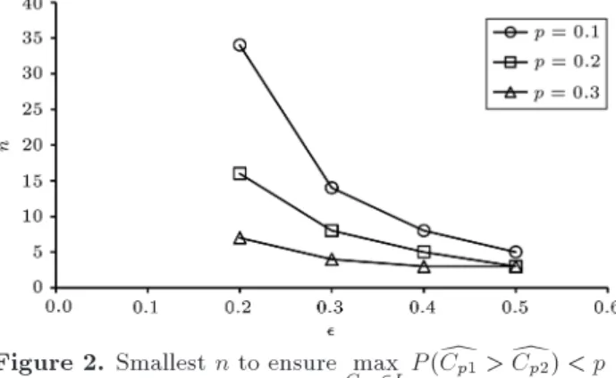
In order to nd the relation between n and , we provide Figures 1 and 2 constructed from Tables 1 to 3. It is seen that n is a decreasing function of . Without any surprises, the reasons are as follows. For Cp1 2 L [ R = (0; (1 )Cp2] [ [(1 + )Cp2; 1),
increasing will increase jCp1 Cp2j, thereby increase
jdCp1 Cdp2j, since dCp1 and dCp2 are close to Cp1 and
Cp2, respectively. Large value of jdCp1 Cdp2j will make
fdCp1> dCp2g easy to observe when Cp12 R and make
fdCp1 > dCp2g hard to observe when Cp12 L. In other
words, large correspond to small sample size n needed to make P (dCp1 > dCp2) large when Cp1 2 R and make
P (dCp1> dCp2) small when Cp12 L.
Figure 1. Smallest n to ensure min
Cp12RP (dCp1> dCp2) > p
with R = [(1 + )Cp2; 1).
Figure 2. Smallest n to ensure max
Cp12LP (dCp1> dCp2) < p
with L = (0; (1 )Cp2]. 4. Remarks
In this section, we will discuss some connections be-tween our method and condence interval and unbiased estimators.
In addition to our comparison method, condence intervals for Cp1 Cp2 can also be applied to make
comparisons between bCp1 and bCp2. We will show that
these two methods are equivalent when sample size is large. But, our method is better when sample size is small.
Our approach depends heavily on the maximum likelihood estimators of the standard deviations. Since the maximum likelihood estimators are biased, it is interesting to see the eects when the maximum like-lihood estimators are replaced by some other unbiased estimators. We will show that estimators might make no dierence for the comparisons.
First, we present the connection to condence interval. When sample size n is large, it is known by central limit theorem that bCp1 and bCp2 are
asymp-totically normally distributed as N(Cp1;2n1 Cp12 ) and
N(Cp2;2n1Cp22 ), respectively (see [19]). Therefore,
b
Cp1 Cbp2 is asymptotically normally distributed as
N(Cp1 Cp2;2n1 [Cp12 + Cp22 ]), since bCp1 and bCp2 are
independent. Consequently, an approximately level (1 )% of condence interval for Cp1 Cp2 is given
as [A; B], where: A = bCp1 Cbp2 z=2
s b C2
p1+ bCp22
2n ;
B = bCp1 Cbp2+ z=2
s b C2
p1+ bCp22
2n ;
and z=2satises P (N(0; 1) z=2) = =2.
We conclude that Cp1> Cp2when:
b
Cp1 Cbp2 z=2
s b C2
p1+ bCp22
2n > 0: Thus, we want:
P 0
@ bCp1 Cbp2 z=2 s
b C2
p1+ bCp22
2n > 0 1 A ; to be large (small) when Cp1> (<)Cp2.
Similarly, we conclude that Cp1< Cp2 when:
b
Cp1 Cbp2+ z=2
s b C2
p1+ bCp22
2n < 0: Thus, we want:
P 0
@ bCp1 Cbp2+ z=2 s
b C2
p1+ bCp22
2n < 0 1 A ; to be large (small) when Cp1< (>)Cp2.
When n is large, z=2
q
b C2
p1+ bCp22
2n is negligible, and
condence interval based comparison method needs P ( bCp1 Cbp2 > 0) to be large (small) when Cp1 >
(<)Cp2, equivalent to our method.
When sample size n is small, it is not easy to nd a condence interval for Cp1 Cp2, since the distribution
of bCp1 Cbp2 is extremely complicated. Clearly, our
method works well for small n, and hence better than condence interval based comparison.
We proceed to present the connection to unbiased estimators. First, consider the unbiased estimator constructed from sample standard deviation. Let:
Sj =c1
4
sPn
i=1(Xji Xj)2
(n 1) ; j = 1; 2;
where: c4=
r 2 n 1
(n=2) ((n 1)=2):
Then, Sj is an unbiased estimator of j; j = 1; 2
(see [20]). Dene:
Cpj= USL LSL6 S
j ; j = 1; 2:
Then:
P Cp1> Cp2= P S2> S1
= P (S2> S1) = P
b
Cp1> bCp2
: Consequently, the nal comparisons results made by maximum likelihood estimators S1 and S2 will be the
same as using unbiased estimators S1 and S2.
Sample range can also be modied to be un-biased estimator of the standard deviation. De-ne Xj(n) = maxfXj1; Xj2; ; Xjng, and Xj(1) =
minfXj1; Xj2; ; Xjng, then Rj = Xj(n) Xj(1)
denotes the sample range of Xj1; Xj2; ; Xjn; j =
1; 2. Dene: ~
Sj =Rdj 2;
where d2 = ERjj, then ~Sj is an unbiased estimator of
j, j = 1; 2: Note that d2 depends only on the sample
size (see [20]). Dene: ~
Cpj= USL LSL6 ~S
j ; j = 1; 2:
Then:
PC~p1> ~Cp2
= PS~2> ~S1
= P (R2> R1):
When sample size n is large enough, Rj will be close
to 4Sj, denoted by Rj 4Sj; j = 1; 2. In this case:
PC~p1> ~Cp2
= P (R2> R1) P (4S2> 4S1)
= P (S2> S1) = P
b
Cp1> bCp2
: Therefore, the nal comparisons results produced by S1 and S2 will be close to those results made by ~S1
and ~S2.
However, when Rj is not close to 4Sj, j = 1; 2;
it is extremely dicult to calculate P (R2 > R1) and
P ( ~Cp1 > ~Cp2) exactly. The evaluation of P ( ~Cp1 >
~
Cp2) and the subsequent work for comparison deserves
a future research. More topics for future study are presented in the following section.
5. Future study
In this paper, we deal with one-dimensional process capability index Cp comparisons based on maximum
likelihood estimators constructed from two normal distributions. There are many ways to extend our ndings. We point out below some directions for future research.
Extension from Cp comparison to Cpk comparison:
Let and denote the process mean and standard deviation, respectively. The process capability index Cpk is dened as d j Mj3 where d = USL LSL2
and M = USL+LSL
2 . Index Cpk was created to
oset some of the weakness of Cp, primarily the
fact that Cp measured capability in terms of
pro-cessvariation only and did not take process location into consideration [3]. Therefore, it is valuable to make Cpk comparison when the mean values of
the processes are o-target. Let bCpk1 and bCpk2
obtained from two normal processes. The complex distribution of bCpk1 Cbpk2will make the evaluation
of P ( bCpk1 Cbpk2> 0) extremely dicult. Numerical
or simulation techniques may be helpful to solve this problem.
Extension from Cp comparison to multivariate Cp
comparison: Let and denote the process mean vector and variance-covariance matrix, respectively; and multivariate Cp can be dened based on jj or
tr, the determinant, and trace of , respectively. Based on observations sampled from multivariate normal distribution N(; ), comparison can be based on j^j or tr^, where ^ is the maximum likelihood estimator of . Multivariate Cp
compar-ison can be made based on many mathematical and statistical properties of ^ provided in [21].
Multivariate Cp can also be dened by:
CpM =
Pv
i=1(USLi LSLi)
Pv
i=1(UPLi LPLi);
where USLi and LSLi are the upper and lower
specication limits for the ith quality characteristic; UPLi and LPLi are the upper and lower
speci-cation limits of a modied process region for the ith quality characteristic, i = 1; ; v (see [22] for more details). In this case, we may need help from computer software since the mathematical framework is hard to deal with.
Extension from normal process comparison to non-normal process comparison: Non-non-normal observa-tions are frequently found from many processes in industry, for instances, leukocyte ltering pro-cess [23] and manufacturing propro-cess [24], among others. If non-normal process can be transformed to normal via the Box-Cox transformation [25], then the Cp comparison method for normal processes
can be applied. If the Box-Cox transformation is not successful, we seek help from the denition of Cp suitable for non-normal process. For example,
quantile based CP denitions can be found in
[26-28], among others. However, the estimation of Cp is then formed from quantile estimators. It
is not easy to make inferences based on quantile estimators since the distributions involved are very complicated.
Extension from two-process comparison to three-process comparison: Given maximum likelihood estimators bCp1; bCp2, and bCp3 obtained from three
normal processes, we can make three comparisons based on f bCp1; bCp2g, f bCp1; bCp3g, and f bCp2; bCp3g,
separately, from which conclusion can be made. Alternatively, we can also make one comparison based on bCp1; bCp2, and bCp3 simultaneously. In
this case, the calculation of P ( bCp1 > bCp2 > bCp3)
and the subsequent settings for comparison are straightforward and tedious.
6. Conclusions
Let X1 and X2 be two manufacturing processes with
process capability indices Cp1 = USL LSL61 and Cp2 = USL LSL
62 , respectively. Let dCp1 and dCp2 denote the maximum likelihood estimators of Cp1 and Cp2 under
the normality assumption. We calculate P (dCp1> dCp2)
and present a table from which smallest sample sizes can be determined to make minCp12RP (dCp1 > dCp2) large and make maxCp12LP (dCp1 > dCp2) small, where L = (0; (1 )Cp2]; R = [(1 + )Cp2; 1), and > 0.
Consequently, comparison of Cp1 and Cp2 based on
d
Cp1 and dCp2 provide manufacturers and consumers a
way to correctly (wrongly) recognize better suppliers to cooporate and better merchandise to purchase, respectively, with high (low) probability. We discuss statistical properties concerning our method. We also point out some directions for future study.
Acknowledgments
The authors appreciate Editor-in-Chief and referees for their valuable comments. According to referees' recommendations, Sections 4 and 5 are created thereby broadening the contributions of this paper.
References
1. Lu, X. and Liu, Z. \Process capability analy-sis of higher education", www.seiofbluemountain.com (2009).
2. Alejandro, R.G., Javier, T.N. and Giner, A.H. \IKS index: A knowledge-model driven index to estimate the capability of medical diagnosis systems to produce results", Expert Systems with Applications, 40(17), pp. 6798-6804 (2013).
3. Kotz, S. and Lovelace, C.R., Process Capability Indices in Theory and Practice, Oxford University Press Inc, London (1998).
4. Kane, V.E. \Process capability indices", Jouranal of Quality Technology, 18(1), pp. 41-52 (1986).
5. Finley, J.C. \What is capability? Or what is Cp
and Cpk", ASQC Quality Congress Transactions,
Nashville, pp. 186-191 (1992).
6. Montgomery, D.C., Introduction to Satistical Quality Control, 2nd Ed., John Wiley and Sons, New York (1991).
7. Kotz, S. and Johnson, N.L., Process Capability Indices, Chapman and Hall, London (1993).
8. Bothe, D.R., Measuring Process Capability, McGraw-Hill (1997).
H.E. \Modied multivariate process capability index using principal component analysis", Chinese Journal of Mechanical Engineering, 27(2), pp. 249-259 (2014). 10. Hosseinifard, S.Z. and Abbasi, B. \Evaluation of pro-cess capability indices of linear proles", International Journal of Quality & Reliability Management, 29(2), pp. 162-176 (2012).
11. Ebadi, M. and Amiri, A. \Evaluation of process capa-bility in multivariate simple linear proles", Scientia Iranica, Transaction E: Industrial Engineering, 19(6), pp. 1960-1968 (2012).
12. Noorossana, R., Eyvazian, M. and Vaghe, A. \Phase II monitoring of multivariate simple linear proles", Computers and Industrial Engineering, 58(4), pp. 563-570 (2010).
13. Chan, L.K., Cheng, S.W. and Spiring, F.A. \The robustness of the process capability index to de-partures from normality", In Statistical Theory and Data Analysis II (Proc. Second Pacic Area Statistical Conference), Tokyo, pp. 223-239 (1988).
14. Chou, Y. and Owen, D.B. \On the distribution of the estimated process capability indices", Communi-cations in Statistics: Theory & Methods, 18(12), pp. 4549-4560 (1989).
15. Chou, Y., Owen, D.B. and Borrego, S.A. \Lower con-dence limits on process capability indices", Journal of Quality Technology, 22(3), pp. 223-229 (1990). 16. Li, H., Owen, D.B. and Borrego, S.A. \Lower
con-dence limits on process capability indices based on the range", Communications in Statistics-Simulation and Computation, 19(1), pp. 1-24 (1990).
17. Pearn, W.L. and Kotz, S., Encyclopedia and Handbook of Process Capability Indices, World Scientic (2006). 18. Hogg, R.V. and Craig, A.T., Introduction to
Mathe-matical Statistics, 5th Ed., Prentice Hall (1995). 19. Chen, S.M., Hsu, Y.S. and Pearn, W.L.
\Capabil-ity measures for m-dependent stationary processes", Statistics, 2(37), pp. 145-168 (2003).
20. Montgomery, D.C., Satistical Quality Control, 7th Ed., John Wiley and Sons, New York (2013).
21. Anderson, T.W., An Introduction to Multivariate Sta-tistical Analysis, 2nd Ed., John Wiley and Sons, New York (1984).
22. Hubele, N.F., Shahriari, H. and Cheng, C.S. \A bivariate process of capability vector", In Statistical Process Control in Manufacturing, Keats, J.B. and Montgomery, D.C., Eds., Marcel Dekker, New York, pp. 299-310 (1991).
23. Hosseinifard, Z., Abbasi, B. and Niaki, S.T.A. \Process capability estimation for leukocyte ltering process in blood service: A comparison study", IIE Transactions on Healthcare Systems Engineering, 4(4), pp. 167-177 (2014).
24. Abbasi, B. \A neural network applied to estimate pro-cess capability of non-normal propro-cesses", Expert Sys-tems with Applications, 2(36), pp. 3093-3100 (2009).
25. Hosseinifard, S.Z., Abbasi, B., Ahmad, S. and Abdol-lahian, M. \A transformation technique to estimate the process capability index for non-normal processes", The International Journal of Advanced Manufacturing Technology, 40(5), pp. 512-517 (2008).
26. Clements, J.A. \Process capability indices for non-normal calculations", Qual. Prog., 22, pp. 49-55 (1989).
27. Chen, L.K., Cheng, S.W. and Spiring, F.A. \A graph-ical technique for process capability", ASQC Quality Cong. Trans. Dallas, pp. 268-275 (1988).
28. Choi, I.S. and Bai, D.S. \Process capability indices for skewed populations", Proc. 20th Int. Conf. on Computer and Industrial Engineering, pp. 1211-1214 (1996).
Appendix
Here, we calculate Eqs. (5), (6), and (7) stated in Section 2. First note that S2221
S2
122 has an F distribution, F (n 1; n 1), with probability density function:
(n 1)
n 1
2
2 w (n 3)=2
(1 + w)n 1; 0 < w < 1; (A.1)
(see [18]).
In view of Relation (A.1) with the transformations w = (tan )2 and t = 2, we have:
PCdp1> dCp2
= P (S2
2 > S12)
= P
S2 221
S2 122 >
2 1 2 2 = P
Fn 1;n 1> 2 1 2 2 = 1 Z 2 1=22
(n 1)
n 1
2
2 w
(n 3)=2
(1 + w)n 1dw
= =2 Z (n 1) n 1 2
2[(tan )
2](n 3)=2
[1+(tan )2]n 1:[2 tan ][sec ]2d
=2 (n 1)n 1
2
2
=2
Z
(tan )n 2
(sec )2n 4d
= (n 1)
2n 2 n 1 2
2
Z
2
(sin t)n 2dt;
where = tan 1(
We will calculate Eq. (5) further for n = 2k + 3 and n = 2k + 2 separately, where k 2 f0; 1; 2; g. Consider the case when n = 2k + 3: To show Eq. (6), combine Eq. (5), the transformation u = cos t, and binomial theorem together to imply that:
PCdp1> dCp2
= (n 1)
2n 2 n 1 2
2
Z
2
(sin t)n 2dt
= (n 1)
2n 2 n 1 2
2
Z
2
(sin t)2k+1dt
= (n 1)
2n 2 n 1 2
2 cos(2)Z
1
(1 u2)kdu
= (n 1)
2n 2 n 1 2 2: cos(2)Z 1 k X i=0 k i
( u2)idu
= (2k + 2)
22k+1[ (k + 1)]2
:
k
X
i=0
( 1)ik
i
[cos(2)]2i+1+ 1
2i + 1 ;
where cos(2) =22 21
2
1+22; as was shown.
We proceed to calculate Eq. (5) with n = 2k + 2 and verify Eq. (7). First note that integration by parts implies:
Z
(sin t)mdt = (sin t)m 1(cos t)
m
+m 1
m Z
(sin t)m 2dt; (A.2)
where m 2 is a positive integer. Applying Eq. (A.2) several times, we have:
PCdp1> dCp2
= (n 1)
2n 2 n 1 2
2
Z
2
(sin t)n 2dt
= (n 1)
2n 2 n 1 2
2
Z
2
(sin t)2kdt
= (n 1)
2n 2 n 1 2
2
"
(sin 2)2k 1(cos 2)
2k
+2k 1 2k
Z
2
(sin t)2k 2dt
#
= (n 1)
2n 2[ (n 1 2 )]2
(
(sin 2)2k 1(cos 2)
2k +(2k)(2k 2)2k 1 (sin 2)2k 3(cos 2)
+(2k 1)(2k 3) (2k)(2k 2)
Z
2
(sin t)2k 4dt
)
= (n 1)
2n 2[ (n 1 2 )]2
(
(sin 2)2k 1(cos 2)
2k +(2k)(2k 2)2k 1 (sin 2)2k 3(cos 2)
+ (2k 1)(2k 3)
(2k)(2k 2)(2k 4)(sin 2)2k 5(cos 2)+ +(2k)(2k 2)(2k 4) 2(2k 1)(2k 3) 3 (sin 2)(cos 2) +(2k)(2k 2)(2k 4) 2(2k 1)(2k 3) 3:1
Z
21dt
)
= (2k + 1)
22k 2k+1 2
2
(
(sin 2)2k 1(cos 2)
2k +(2k)(2k 2)2k 1 (sin 2)2k 3(cos 2)
+(2k)(2k 2)(2k 4)(2k 1)(2k 3) (sin 2)2k 5(cos 2)+
+(2k)(2k 2)(2k 4) 2(2k 1)(2k 3) 3 (sin 2)(cos 2) + (2k 1)(2k 3) 3:1
(2k)(2k 2)(2k 4) 2( 2) )
; where = tan 1(1=2); sin 2 = 212
2
1+22, and cos 2 =
2 2 21
2
1+22. The verication is completed. Biographies
Sy-Mien Chen received her PhD degree from De-partment of Mathematics, University of Maryland at College Park, in 1990. She is currently an Asso-ciate Professor at Department of Mathematics, Fu-Jen
Catholic University, Taiwan. Her research interests are statistics and statistical quality control. Her papers are mainly published at Statistics, Journal of Nonparamet-ric Statistics, Communication in Statistics, and Fu-Jen Studies.
Jian-Tong Liaw received his PhD from Institute tute of Applied Science and Engineering, Fu-Jen Catholic University in 2008. He is currently an Assistant Professor at Fu-Jen Catholic University, Taiwan. His research interests are statistics and its applications and computational statistics. He has published papers at
Statistics, Fu-Jen Studies, and Journal of Probability, and Statistical Science.
Yu-Sheng Hsu received his PhD degree from De-partment of Statistics, Rutgers University, in 1990. He is currently an Associate Professor at Department of Mathematics, National Central University, Taiwan. His research elds include statistics and its applica-tions. He has published papers at Statistics, Journal of Nonparametric Statistics, Communication in Statis-tics, IEEE Sensors Journal, and IEEE Transactions on Antennas and Propagation.