Sharif University of Technology
Scientia IranicaTransactions E: Industrial Engineering www.scientiairanica.com
Network revenue management under specic choice
models
F. Etebari
a;, A. Aghaei
aand A. Jalalimanesh
ba. Department of Industrial Engineering, K.N. Toosi University of Technology, Tehran, P.O. Box 1999143344, Iran.
b. Department of Information Engineering, Iranian Research Institute for Information Science and Technology, 1090, Enqelab Ave., Tehran, P.O. Box 13185-1371, Iran.
Received 14 March 2012; received in revised form 17 April 2013; accepted 11 May 2013
KEYWORDS Competition, multinomial logit model (MNL); Independence of Irrelevant Alternatives (IIA);
Nested logit model; Column generation subproblem.
Abstract.New challenges in the business environment, such as increased competition and the inuence of the Internet on main distribution channels has led to fundamental changes in traditional revenue management models. Under these conditions, modeling individual decisions more accurately is becoming a key factor. Nearly all research studies about choice-based revenue management models use the well-known multinomial logit model. This model has one important restriction, that is, the independence of irrelevant alternatives; a property which states that the ratio of choice probabilities for two distinct alternatives is independent of the attributes of any other alternatives. In this paper, a nested logit model is proposed for removing this limitation and incorporating a correlation between alternatives in each nest. The new subproblem of column generation is introduced and a combination of heuristic and metaheuristic algorithms for solving this problem is provided. Interesting outcomes are obtained during analysis of the results of experimental computations, such as oer sets and iteration trends, with respect to the correlation measure inside each nest. Simulation results show that, although changing the choice model might lead to signicant improvement in revenue under some conditions, during all scenarios, observing the correlation should not cause the choice model to change immediately.
c
2013 Sharif University of Technology. All rights reserved.
1. Introduction
Today's market environment can be explained with several simple words; increased competition pressure, the growing dominance of information technology such as the Internet, and the existence of rich sources about revealed preference data in a mutual environment. At the beginning of the previous decade, it was con-cluded that the assumption of independent demand in traditional models has serious limitations. Revenue management scientists preferred to use a new genera-tion of choice based revenue management structures, including simple and well known choice models, such
*. Corresponding author. Tel.: +98-21-84063482 E-mail address: f [email protected] (F. Etebari)
as the multinomial logit model, for capturing customer behavior and taking into account the eects of buy up, buy down and recapture. The independent demand model uses the assumption that the demand for each fare class is independent from rm availability controls. Then, traditional carriers felt the eects of these factors more seriously and tried to minimize their undesirable eects on their revenue.
All above mentioned factors have resulted in the need for better modeling of individual purchasing decisions. Application of a multinomial logit model to forecast ridership for a new transportation line in 1972, in San Francisco, provided a strong foundation and motivation for researchers to transit from modeling demands using aggregate data to modeling demands as a collection of individual choices. Nowadays, with the
growth in online shopping and booking, there is a new rich source of data to model customer preferences.
Cooper et al. (2006) show that if an airline wants to decide about the number of seats that should be reserved for sale at a high-fare, based on the sales history, while neglecting to account for the fact that the availability of low-fare tickets will reduce high-fare sales, then, high-fare sales will decrease, resulting in a lower future estimation of high-fare demand. This process is called the spiral-down eect and is observed only if historical data is used for demand forecasting. There are dierent reasons, such as those mentioned above, for using discrete choice models in order to forecast future demand.
The most popular choice model is the multino-mial logit model (MNL). Despite its simplicity and eciency, this model has some restrictions. The most important limitation of the MNL model is the assumption of the independent distribution of utility function errors across alternatives, which leads to the Independence of the Irrelevant Alternatives (IIA) eect. This property states that the ratio of choice probabilities is independent of the attributes of any other alternatives.
The property of IIA, which may not be a realistic assumption, means that a change or improvement in the utility of one alternative will draw shares propor-tionally from all other alternatives. For instance, in parallel ights, it is expected that a ight departing in the afternoon competes further with other afternoon departing ights.
Schon (2010) states that, recently, much attention has been given to (a) modeling how consumers choose among a set of multiple products, and (b) accommo-dating the realistic discrete choice model of consumer behavior in normative RM, while keeping problem complexity at a reasonable level, simultaneously. The nested logit model incorporates more realistic substi-tution patterns by relaxing the assumption of indepen-dent distribution of errors and grouping alternatives to the dierent nests.
The organization of this paper is as follows. In Section 2, a brief literature review of the related works is described. In Section 3, the Choice-based Deter-ministic Linear Programming (CDLP) approach and nested logit models are explained. At the beginning of section four, the column generation algorithm is described, and, subsequently, a new subproblem of this algorithm, based on the nested logit model, is proposed. In the rest of this section, a new approach, com-posed of heuristic and genetic algorithms, is introduced for solving the problem. In the next section, a complete test problem is modeled and solved by with the aid of the proposed method, and the results are illustrated using a simulation of customer behavior with test problem data. The last section includes the discussion
and conclusion, and nally, a number of interesting topics are presented for future research.
2. Literature review
Most traditional revenue management models are based on an independent demand assumption. A complete survey of traditional revenue management models can be found in Talluri and Van Ryzin [1]. Belobaba and Hopperstad [2] show the importance of considering customer choice decision behavior. They studied passenger purchase behavior using simulation for analyzing the sensitivity of airline time, date, path and price to passenger preferences. Anderson [3] and Algers and Baser [4] report the results of a project in the Scandinavian Airlines System (SAS) regarding estimation of recapture and buy up using stated and revealed preference data.
Zhang and Cooper [5] used the Markovian deci-sion process for simultaneous seat-inventory control of a set of parallel ights from common origins to common destinations, considering customer choice among the ights. Their model assumes that the customer chooses within the same fare class among dierent ights but not between fare classes. They proposed heuristics and simulation-based techniques for solving this problem, and also applied a general choice model for considering customer behavior.
Van Ryzin and Vulcano [6] consider the network capacity control problem, where customers choose among various products oered by a rm. They model customer choice, assuming that each of them has an ordered list of preferences. They assume that the rm controls the availability of products using a virtual nesting control strategy.
Chen and Homem-de-Mello [7] consider network airline revenue management, when the customer choice model is based on the concept of preference orders. They proposed a new model using mathematical pro-gramming techniques to determine seat allocation.
Talluri and Van Ryzin [8] provide a complete characterization of an optimal policy under a general discrete choice model of customer behavior in a single leg revenue management model. They illustrate that an optimal policy is made up of a selected set of ecient oer sets, where these sets are a sequence of no dominated sets providing the highest positive exchange between expected capacity assumption and expected revenue.
Gallego et al. [9] provide a customer choice-based LP model for network revenue management. They sup-pose that the rm has the ability to provide customers alternative products to serve the same market demands with a exible product oering. One limitation of their market demand model is that it does not allow any kind of segmentation.
Liu and Van Ryzin [10] use the analysis of the model provided by Gallego et al. [9] to extend the concept of ecient sets. They prove that when capacity and demand are scaled up proportionally, revenue obtained under choice-based deterministic linear pro-gramming converges to the optimal revenue under the exact formulation. They present a market segmenta-tion model to describe choice behavior. The segments are dened by disjoint consideration sets of products, where a consideration set is a subset of the products provided by the rm, which customers consider options. Bront et al. [11] extended the work of Liu and Van Ryzin [10] by allowing the customers to consider products which belong to overlapping segments. In this case, they proved that the column generation subproblem is Np-hard and proposed a greedy heuristic to solve it.
Kunnukal and Topaloglu [12] proposed a new deterministic linear program for the network revenue management problem with customer choice behavior. They generated bid prices that depended on the time left until the time of departure. The main drawback of their model is that the number of constraints in their model is signicantly larger than linear programming formulation used by Liu and Van Ryzin [10].
Vulcano et al. [13] developed a maximum likeli-hood estimation algorithm in discrete choice models for airline revenue management. Their simulation results show 1%-5% average revenue improvements using choice-based revenue management.
For analyzing the eects of applying mis-specied models, Amaruchkul and Sae-Lim [14] studied the static overbooking models. They assume that the decision model embedded in a commercial revenue management system is mis-specied. They explore the consequences of the modeling error and nd that the performance of the model with mis-specication de-creases as show-up probability dede-creases. Meissner and Strauss [15] propose a new heuristic for specifying bid prices in a choice-based network revenue management problem.
Derigs and Friederichs [16] propose a decision support system for maximizing the revenue generated in the area of waste and row material management. They use the dual variables of the linear program for setting bid prices. Schutze [17] applies price-based revenue management for hotel room pricing. Dierent pricing strategy clusters are proposed according to the hotel category.
Ben-Akiva and Lerman [18] analyzed dierent discrete choice models. Train [19] provided the most advanced elements of the estimation and usage of discrete choice models that require simulation. Garrow [20] provided a comprehensive overview of discrete choice models and application of these models to the airline industry.
Garrow et al. [9] completed the study of air-line traveler no-show and standby behavior, based on passenger and directional outbound/inbound itinerary data. They focus on passenger behavior based on the estimation of a multinomial logit model and de-scribe the benets of using passenger data to improve forecasting accuracy and to support a broad range of managerial decisions.
3. Model
Consider a network with m resources (legs) providing n products. N = f1; 2; ; ng denotes the set of products and rj is the associated revenue (fare)
for product j 2 N. We study capacity usage by dening vector c = (c1; c2; ; cm), which denotes the
initial capacities of resources (legs). Resource usage, according to the corresponding product, is presented by dening an incidence matrix, A = [aij] 2 Bmn.
The matrix entries are dened by aij = 1, if resource
j is used by product j and aij = 0 otherwise. Aj,
the jth column of A, denotes the incidence vector for product j, and notation i 2 Aj indicates that product
j is using resource i. Note that one product can use more than one resource. Time has discrete periods and runs forward until a nite number, T ; t = 1; 2; ; T , and it is assumed that we have, at most, one arrival for each period of time, and that each customer can buy only a single product.
We divide customers into L dierent segments. A consideration set, Cl N, l = 1; 2; ; L is
used to describe each segment. Gallego et al. [9] consider a unique segment C1 = N, Liu and Van
Ryzin [10] represent non overlapping segments where Cl\ Cl0 = ;, for all l 6= l0, and nally, Bront et al. [11] consider overlapping segments, where Cl \ Cl0 6= ;, for certain l 6= l0. We are going to analyze a model
that has dierent nests in each segment. Alternatives that belong to the same nest, share common errors, whereas alternatives that are in dierent nests have independent errors. In this paper, we hypothesized the alternatives which are grouped share common, unobserved attributes. These unobserved attributes cannot be incorporated into the observed portion of the utility.
If we have one arrival, pl represents the
proba-bility that an arriving customer belongs to segment l, with PLl=1pl = 1. We consider a Poisson process of
arriving streams of customers from segment l, with rate l= pland total arriving rate of =
L
P
l=1l.
In each period of time t, the rm should decide about its oer set (i.e. a subset S N of products that the rm makes available for customers). If set S is oered, the deterministic quantity Pj(S) indicates the
otherwise. Using the probability law, we have: X
j2S
Pj(S) + P0(S) = 1;
where P0(S) indicates the no-purchase probability.
3.1. Customer choice model
To model customer choice behavior, we can assume that each customer wants to maximize his utility, while his utility for alternatives is a random variable. The rm is oering a set of alternatives for customer n, where he/she has a consideration set, Cn with
utility Uin for each alternative, i 2 Cn. This utility
can be decomposed into two deterministic (also called expected utility); denoted in, and a mean-zero random
component "in without loss of generality. Hence, we
have a utility function as follows:
Uin= in+ "in: (1)
In many cases, the representative component, in, is
modeled as a linear combination of several attributes:
in= Txin; (2)
where is an unknown vector of weights that should be computed from data and xinis the vector of observable
attributes for alternative i available to customer n at the time of purchase, such as time and date of departure, price, departure airport, airline brand, and so on.
Train [19] states that one of the best and most commonly used models for studying how customers make their choice is the multinomial logit (MNL) model. In this model it is assumed that the "in in
the utility functions are independent and identically-distributed random variables with a Gumbel distri-bution. The probability whereby customer n chooses alternative i 2 Cn in a MNL model is given by:
Pn(i) = e Tx
in P
j2Cn
eTxjn+ 1: (3)
Based on Garrow (2010), the Nested Logit (NL) model, which appeared just a few years after the MNL model, incorporates more realistic substitution patterns by relaxing the assumption that errors are independent. Within the airline industry, there are many applica-tions in which the NL model can oer forecasting benets over the MNL model. For each nest, the logsum parameter, m, is a measure of the degree of
correlation and substitution among alternatives in nest m. A higher value of mimplies less, and lower values
imply more correlation among alternatives in the nest. In fact, higher correlation leads to greater competition eects among alternatives in the nest.
In the nested logit model, the probability that
individual n selects alternative i is given by:
Pj(S) =
eVj=m "
P
i2Am eVi=m
#m 1
M
P
l=1
" P
i2Al eVi=l
#l ; 0 < m 1: (4) A more intuitive expression for the NL choice probabil-ity can be derived as the product of a conditional and marginal probability.
Pj = Pjjm Pm= e Vj=m P
i2Am
eVi=m
eVm+m m
M
P
l=1e Vl+l l
;
0 < m 1; (5)
m= ln
" X
i2Am eVi=m
#
; 0 < m 1: (6)
The rst component of the product is the probability of selecting alternative j among all i alternatives in nest m, conditional to the choice of m, and the second product is the probability of selecting nest m among all nests. m is often called the \log-sum term" because
it is the log of a sum.
3.2. Dynamic and linear programming models In the general case, as a rm cannot recognize the corresponding segment of an arrival in advance, we consider Pj(S); the probability whereby the rm sells
product j to an arriving customer as: Pj(S) =
L
X
l=1
plPlj(S): (7)
In this equation, Plj(S) represents the probability of
choosing product j by a customer who belongs to segment l. The expected revenue, by oering set S N for an arriving customer is given by:
R(S) =X
j2S
rjPj(S): (8)
Given that we oer set S, let P (S) = (P1(S); ; Pn(S))T be the vector of purchase
probabilities and A the incidence matrix of resources used by products. Then the vector of capacity consumption probabilities Q(S) is given by:
Q(S) = A:P (S); (9)
where Q(S) = (Q1(S); ; Qm(S))T, and Qi(S)
indi-cates the probability of using a unit of capacity on leg i, i = 1; 2; ; m: Based on Liu and Van Ryzin [10]
this problem can be formulated as a dynamic program problem:
Vt(x) = max SN
8 < :
X
j2S
Pj(S)(rj+ Vt+1(x Aj))
+ (P0(S) + 1 )Vt+1(x)g
= max
SN
8 < :
X
j2S
Pj(S)(rj (Vt+1(x)
Vt+1(x Aj)))g + Vt+1(x); (10)
and the boundary conditions are Vt(0) = 0; t =
1; 2; ; T and VT +1(x) = 0; 8x 0. Since the state
space is multi dimensional, this problem is intractable and is approximated with a linear programming.
The rm's decision consists of deciding which set of products should be oered at any period of time t, while it cannot distinguish each customer related segment in advance. However, as choice probabilities are time-homogeneous and demand is deterministic, it only matters how many times each set S is oered; knowing during exactly which period is not important. The variable t(S) represents the number of periods during which set S is going to be oered. Another assumption is that we let variable t(S) be continuous as well (i.e. the rm could oer a set S for a whole or a fraction of a period of time). The model's objective is to maximize rm revenue by deciding the number of periods of time for each set of products. Formulation of the CDLP problem will be:
VCDLP= maxXR(S)t(S):
S.t. X
Q(S)t(S) C; X
t(S) T;
t(S) 0; 8S N: (11)
Liu and Van Ryzin [10] prove that since demand and capacity are scaled up proportionately, the revenue obtained under the CDLP model is asymptotically optimal for the original stochastic network choice model.
4. Using column generation to solve the CDLP model
In the model (11), there are an exponential number of primal variables. This means that a problem with
n products, has 2n 1 possible non-empty subsets of
products of set N. In spite of an enormous number of variables for practical real world problems which makes it impossible to enumerate all oer sets, there are at most m + 1 constraints. Gallego et al. [9] represent the idea of using a column generation technique to solve real world practical problems.
The rst step in applying a column generation al-gorithm starts by solving reduced linear programming; that is, just considering a limited number of columns (subsets) indicated by N = fS1; S2; ; Skg. This
takes us to the reduced CDLP model as follows: VCDLP R= maxXR(S)t(S):
S.t. X
Q(S)t(S) C; X
t(S) T;
t(S) 0; 8S N: (12)
Let 2 Rm be the dual prices for the rst
m-dimensional capacity constraints and 2 R be the dual price for the one-dimensional time constraint. Now for the next step in column generation, we construct a column generation subproblem to nd the next column with the most positive reduced cost to add to our set collection, N, which is not included yet. This column is obtained by solving the following sub problem:
max
SN
R(S) TQ(S)
= max
SN
R(S) TQ(S) : (13)
Afterwards, to explicit Eq. (13), a binary vector, y 2 Bn, is dened as follows. Suppose a set, S, is
oered now, then we denote: yj =
(
1; if j 2 S
0; otherwise (14)
A nesting structure of products can be determined in two general dierent ways, according to a no-purchase alternative. The rst approach is to divide products in such a way whereby the no-purchase alternative is placed in the one nest, and all rms' products are allocated in another nest. In this condition, problem (13) can be expressed as follows:
max
y2f0;1gn ( L
X
l=1
max y2f0;1gn 8 > < > : L P l=1l P
j2Cl(rj ATj)eVlj=myj
" P
i2Bm
eVli=m+1=m im eVl0=m
#m 1 M P k=1 " P i2Bk
eVli=kyi+1=kik eVl0=k#k
9 > = >
; ; 0 < 1, (16)
Box I.
P
j2Cl(rj ATj)eVlj=myj "
P
i2Bm eVli=m
#m 1
M P k=1 " P i2Bk
eVli=kyi #k
)
; 0 < 1: (15)
Another approach is to assume that the no-purchase alternative exists in all nests with the same share. With this denition, the column generation subproblem will be calculated in Eq. (16) as shown in Box I. Or, equivalently:
max
y2f0;1gn ( n
X
j=1
(rj ATj)yj L X l=1 l " P i2Bm
eVli=m+ 1=m
im eVl0=m
#m 1
M P k=1 " P i2Bk
eVli=kyi+ 1=k
ik eVl0=k
#k )
; 0 < 1; (17)
where m is the nest that product j belongs to, and Vl0 > 0; 8l assumes that the denominator is greater
than zero all the time. We assume that the no-purchase alternative belongs to all nests in each segment. We assign the allocation parameter, jk which reects the
extent to which alternative j is a member of nest k. This parameter must be nonnegative: jk 0; 8j; k.
Interpretation is facilitated by having the allocation parameters sum to one over nests for any alternative: P
k jk = 1; 8j. If Problem (15) or (17) have a
positive optimal value, then the optimal solution for the problem will be the next entering column to the reduced primal problem. Then we update the reduced CDLP (12) with the new column, and iterations are continued. Finally, if there is no solution for Problem (15) or (17) with a positive value, then the current solution for the reduced CDLP problem (12) is opti-mal.
4.1. Complexity of the column generation subproblem
0-1 fractional programming problems (15) and (17) can be considered a special case of the sum of ratios
problem with more rmly connected variables. Bront et al. [11] proved that the minimum vertex problem, which is known to be an Np-hard, can be reduced to the 0-1 fractional programming problem with the multinomial logit model. Then, this problem is an Np-hard problem. The multinomial logit model is a special case of the nested logit model in which if m= 1 for all
nests, the nested logit model will be equivalent to the MNL model. Then, Problems (15) and (17) are also Np-hard.
4.2. Solution approaches for the column generation subproblem
In this section, we study dierent solution approaches for the column generation subproblem starting by a heuristic method, followed with a metaheuristic. 4.2.1. Greedy heuristic
The fact that the column generation subproblem is an Np-hard optimization problem, guides us to use an alternative approach, which makes it possible to implement this algorithm in practical problems. Bront et al. [11] propose a greedy heuristic to their own prob-lem with complexity O(n2L), based on the heuristic
proposed by Prokopyev et al. [21] to overcome the complexity of the exact algorithm. We are going to propose a new heuristic inspired by this one.
Comparing local and global optimum results shows that, in most cases where a greedy heuristic stops at local optimum, same products exist in the global optimum with some extras. This fact leads us to insert a Boltzmann operator, after stopping the algorithm. This idea stems from the Simulated Annealing (SA) approach. This heuristic starts with an empty set, S, taking into account the maximum marginal contribu-tion to the current solucontribu-tion, by adding progressively new products to the current set S. If the algorithm cannot nd any column with a positive reduced cost and the new product does not improve the value of the new set, then the Boltzmann operator will be used and the new product will be inserted with a certain probability.
For applying this operator, we should set the number, say N, of iterations and the initial temper-ature, T0, and the nal temperature, T1(T0> T1). We
decrease temperature T after every iteration, usually by proportion (cooling rate). So that, after N iterations, the temperature becomes tN = NT0.
j
1 = arg maxj2S0 1 8 > < > : L P l=1 P
j2Cl\(S[fjg)(rj A T
j)eVlj=m
" P
i2Bm\(S[j)
eVli=m+1=m im eVl0=m
#m 1 M P k=1 " P i2Bk\(S[j)
eVli=kyi+1=k ik eVl0=k
#k 9 > = > ;: Box II.
j= arg max j2S0 1 8 > < > : L P l=1l
P
j2Cl\(S[fjg)(rj A T
j)eVlj=m
" P
i2Bm\(S[j)
eVli=m+1=m im eVl0=m
#m 1 M P k=1 " P i2Bk\(S[j)
eVli=kyi+1=k ik eVl0=k
#k 9 > = > ;: Box III.
(this algorithm has been proposed for Relation (17) and can be adapted with Relation (15) easily):
Step 1: For all product j, such that rj ATj 0,
set yj = 0;
Step 2: Let S0
1 N be the set of products j with
no assigned value for yj;
Step 3: Compute: j
1 = arg maxj2S0 1
( L X
l=1
(rj ATj)
eVlj=m "
P
i2Bm
eVli=m+ 1=m
im eVl0=m
#m 1
M P k=1 " P i2Bk
eVli=kyi+ 1=k
ik eVl0=k
#k )
:
Set S1:= fj1g, S01:= S10 fj1g;
Step 4: Repeat:
Compute the equation given in Box II.
If Value(S1[ fjg) > Value(S1), then S1:= S1[
fjg, and S0
1:= S1 fjg.
Until S1 is not modied.
Step 5: If
L
X
l=1
(rj ATj)
eVlj=m "
P
i2Bm
eVli=m+ 1=m
im eVl0=m
#m 1
M P k=1 " P i2Bk
eVli=kyi+ 1=k
ik eVl0=k
#k
< 0;
for all j 2 S1,
Set yj = 1. For j =2 S1, set yj= 0 and stop;
Else S2:= S1 & S02:= S10 & T0 & T1 & N := 0
and go to the step 6.
Step 6: Repeat:
Compute the equation given in Box III.
Update N := N + 1 tN = N T0 and generate
random number r;
If Value(S2[ fjg) < Value(S2), then compute
Pr ob = exp
Value(S
2[ fjg) Value(S2)
tN
:
If Pr ob > r, then S2 := S2[ fjg, and S20 :=
S0
2 fjg;
Else S1:= S2&S10 := S20 & go back to Step 4.
Until tN T1or Pr ob < r.
Step 7: Stop.
Thus, a new set may be accepted temporarily with some probability if it is inferior compared to the old set. It is easy to see that, initially, when the temperature is high, and the distance from the best set is low, there is a higher probability of accepting an inferior set. This exponential function is called a Boltzmann function, thus, the operation is called a Boltzmann-type operator.
4.2.2. Genetic algorithm
The genetic algorithm was developed by J. Holland in the 1970s to understand the adaptive processes of natural systems [22]. GAs are a very popular class of population-based metaheuristic. These algorithms start from an initial population of solutions. Then, they iteratively generate a new population and replace it with a current population. This replacement is based on selection methods.
One of the most suitable algorithms to tackle the column generation subproblem is the genetic algorithm. According to the nature of this problem, we can transform it to a binary unrestricted problem, this type of which, the GA algorithm successfully solves.
Firstly, the structure of chromosomes is a binary vector with a dimension equal to the number of prod-ucts. A gene of the chromosome, denoted as g(j), where g(j) = 1, means product number j is available in the set, and g(j) = 0, otherwise.
With this chromosome structure, the mutation operator is a uniform function, whose rate is 0.05, whose crossover function is scattered and whose frac-tion rate is 0.8.
This approach rst uses a greedy heuristic in order to identify an entering column to solve the CDLP by column generation. If this algorithm does not nd an entering column, then, we use the metaheuristic GA algorithm. Experiments show that when there is still a column to enter the reduced problem, in most cases, the heuristic will nd it.
The genetic algorithm for solving the column generation subproblem was implemented using the Matlab genetic toolbox.
5. Computational experiment
In this section, we consider a small network for a choice-based network revenue management model with nested segments in which customers choose their products based on a nested logit model.
Taking into account the computational results, we evaluate dierent solution approaches, based on the quality of the obtained solution and computational feasibility. According to the fact that the time com-plexity of the heuristic algorithm is O(n2L), we focus
on analyzing the eect of the correlation of nests in the revenue. For the computational side, we analyze the numbers of iterations and their trend according to the correlation measure in nests.
Mont Carlo simulation has been used for simu-lating customer choice behavior. For analyzing the impact of the correlation between products in each nest, simulation has been done with 1000 streams of demand according to two distinct scenarios:
1. The assumption that customers choose products based on a nested logit model and rms use a standard logit model for determining the required oer sets.
2. The assumption that customers choose products based on a nested logit model and rms apply the nested logit model for determining the required oer sets.
For determining the oer sets in each period, we solve CDLP formulation and determine optimal oer sets
and their related time periods to recommend them. These sets are oered, according to the lexicographic order of the indices of the LP variables. Since variable t(S) could be fractional, we round them to the nearest integer.
Dierent network load factors are tested. To better evaluate the algorithms, we consider dierent capacities by multiplying a load factor, , to the capacity of legs. Parameter is to scale all the legs capacity, where = 1 corresponds to the original base case. The performance in choice behavior is analyzed by varying the no-purchase observed utility vector; V0= (V10; ; VL0). We assume that in each segment,
the no-purchase alternative belongs to all nests, with equal allocation parameters.
5.1. A small airline network
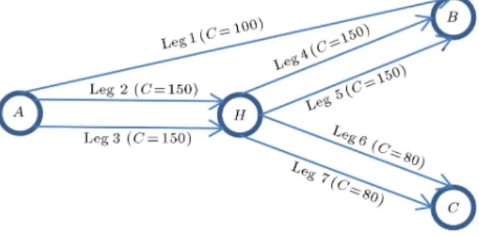
We evaluate dierent heuristic methods and product nesting eects with a small airline network. Consider a network with 4 airports and 7 ight legs. The capacities of the legs are C = (100; 150; 150; 150; 150; 80; 80). The rm oers two high (H) and low (L) fares on each leg. Considering local and connecting itineraries, customers can choose between 22 available products dened by itineraries and fare class combinations. The problem consists of nding a policy which leads us to prepare a set of products at any period of time during the booking horizon to oer to the customers, while the revenue of the rm should be maximized. This airline network is illustrated in Figure 1, and Tables 1 and 2 describe available products in this network.
According to the customer prices and time sen-sitivities, their origin and ultimate destination, 10 overlapping segments and 20 nests (two nests in each segment) are dened in this example. This segmenta-tion is described in Table 2.
The probability of customer arrival for the corre-sponding segment is given in the last column. Columns 3, 4 & 5 specify the nests, their consideration set and the observed utility for the indicated products, respectively.
Indeed, if the capacity of legs exceeds correspond-ing demand, the problem becomes much easier to solve and the rm could oer almost all of its products.
Table 1. Product denition for small network problem. Product Legs Class Fare
1 1 H 1000
2 2 H 400
3 3 H 400
4 4 H 300
5 5 H 300
6 6 H 500
7 7 H 500
8 f2,4g H 600
9 f3,5g H 600
10 f2,6g H 700
11 f3,7g H 700
12 1 L 500
13 2 L 200
14 3 L 200
15 4 L 150
16 5 L 150
17 6 L 250
18 7 L 250
19 f2,4g L 300
20 f3,5g L 300
21 f2,6g L 350
22 f3,7g L 350
To better evaluate algorithms, we consider dierent capacities by multiplying scale factor to the capacity of legs C. We use = 0:6; 0:8; 1; 1:2 & 1.4 to solve the problem and the booking horizon consists of 1000 periods of time.
Table 3 shows the results under the condition whereby the rm uses a nested logit model for deter-mining oer sets, with respect to dierent correlations among alternatives in each nest, dierent load factors and no-purchase observed utility. For a no-purchase utility, we assume that a pair utility is repeated for all segments.
We assume that, correlations in dierent nests are equal. This assumption is considered for better analysis of results and can be relaxed easily.
Table 4 presents similar results when the rm uses a multinomial logit model for specifying oer sets, but customers choose products based on a nested logit model.
Table 5 represents a 95% condence interval for the improvement percent when the rm switches to the nested logit model.
The rst column in the result table is the case in which correlation is zero. We expect these models to have similar results in this condition, due to the fact that when correlation between each nest's alternatives became zero, the nested logit model restructures to a multinomial logit model. It can be observed that in all rows of the rst column of results, the revenue gaps
Table 2. Customer segmentation in small network problem. Segment O-D Nest Con. Set Observed utility 1
1 A-B 1 f1, 8, 9g (2.3000, 2.0800, 2.0800) 0.08 2 f12, 19, 20g (1.7900, 1.3900, 1.3900) 2 A-B 1 f1, 8, 9g (0.0001, 0.6900, 0.6900) 0.2
2 f12, 19, 20g (2.0800, 2.3000, 2.3000)
3 A-H 1 f2, 3g (2.3000, 2.3000) 0.05
2 f13, 14g (1.6100, 1.6100)
4 A-H 1 f2, 3g (0.6900, 0.6900) 0.2
2 f13, 14g (2.3000, 2.3000)
5 H-B 1 f4, 5g (2.3000, 2.3000) 0.1
2 15, 16 (1.6100, 1.6100)
6 H-B 1 f4, 5g (0.6900.0.6900) 0.15
2 f15, 16g (2.3000, 2.0800)
7 H-C 1 f6, 7g (2.3000, 2.0800) 0.02
2 f17, 18g (1.6100, 1.6100)
8 H-C 1 f6, 7g (0.6900, 0.6900) 0.05
2 f17, 18g (2.3000.2.0800)
9 A-C 1 f10, 11g (2.3000.2.0800) 0.02
2 f21, 22g (1.6100, 1.6100)
10 A-C 1 f10, 11g (0.6900, 0.6900) 0.04
Table 3. Revenue results for simulation when rm oers products based on NL model. Small network
Correlation 0 0.2 0.6 0.8
Scale factor
No-purchase
utility Mean %LF Mean %LF Mean %LF Mean %LF
0.6
(0.00, 1.61) 207904.8 93.02054 207993.4 93.11279 206575.9 95.77636 203310.9 94.91705 (1.61, 2.30) 193561.9 93.33527 193447.5 93.31357 185402.0 94.12519 175745.0 96.02054 (2.30, 2.99) 164349.0 93.20271 162821.0 92.94729 155709.2 92.68023 148123.3 92.14690 0.8
(0.00, 1.61) 260799.2 89.15698 259923.4 89.13023 250344.1 92.08547 239459.5 92.82849 (1.61, 2.30) 217825.6 92.25727 216111.5 92.13343 209488.6 92.24448 202329.2 93.25988 (2.30, 2.99) 184764.5 88.60959 183928.0 88.22238 178145.3 86.55349 170175.0 85.69797 1.0
(0.00, 1.61) 276191.2 85.07023 276597.0 84.91302 267626.0 90.21372 258039.2 92.32186 (1.61, 2.30) 230631.4 86.87116 230666.2 88.04605 228506.9 88.47000 224989.9 89.28651 (2.30, 2.99) 190601.9 81.74186 189724.1 81.59651 184409.6 81.00651 175569.4 77.94977 1.2
(0.00, 1.61) 283230.4 75.27558 282294.0 75.06376 277296.8 86.46298 274703.4 88.85891 (1.61, 2.30) 238092.5 74.27287 238249.8 74.27248 236356.0 74.16434 235514.1 76.76899 (2.30, 2.99) 192334.8 70.91589 191800.6 70.80543 185848.2 68.68120 176161.1 65.30640 1.4
(0.00, 1.61) 286072.0 64.62724 285101.8 64.51362 283276.2 74.12907 285054.6 77.78189 (1.61, 2.30) 238194.8 63.64817 238467.5 63.66196 238066.1 63.77824 236551.5 63.67342 (2.30, 2.99) 192401.1 60.85963 191793.6 60.63505 185363.6 58.84302 176349.1 56.04385 Table 4. Revenue results for simulation when rm oers products based on MNL Model.
Small network
Correlation 0 0.2 0.6 0.8
Scale factor
No-purchase
utility Mean %LF Mean %LF Mean %LF Mean %LF
0.6
(0.00, 1.61) 207392.6 92.84031 206979.4 92.58178 199437.8 89.53411 183400.2 82.27647 (1.61, 2.30) 193320.5 93.27984 192556.2 92.99225 181320.9 87.55078 163316.4 78.17519 (2.30, 2.99) 164512.8 93.31395 163366.6 92.99225 152727.3 87.60736 138054.6 79.38527 0.8
(0.00, 1.61) 260940.4 89.18866 260435.0 89.01802 248975.4 85.23895 227128.2 77.54157 (1.61, 2.30) 216355.2 91.93227 216117.6 91.97471 209135.2 90.54942 198589.4 87.73721 (2.30, 2.99) 184212.4 88.38488 183796.6 88.26017 177343.0 85.76638 167133.7 81.12558 1.0
(0.00, 1.61) 276746.8 85.19023 275401.1 84.92884 266761.8 83.36209 249905.2 79.41605 (1.61, 2.30) 230924.5 86.97326 230723.8 86.94163 227675.1 86.73837 222632.8 86.26093 (2.30, 2.99) 190760.8 81.75744 189653.5 81.43767 184303.0 79.62488 174843.1 75.98628 1.2
(0.00, 1.61) 283298.0 75.28566 282916.0 75.48411 276197.0 74.19012 264457.0 72.04981 (1.61, 2.30) 237662.0 74.23760 237861.5 74.23876 236482.7 74.28973 232488.9 73.87132 (2.30, 2.99) 192197.0 70.87403 191727.4 70.76202 185574.7 68.69554 176506.8 65.45543 1.4
(0.00, 1.61) 285996.8 64.69917 285703.2 64.60498 281134.2 64.27193 270573.4 62.90166 (1.61, 2.30) 238691.1 63.67924 238940.1 63.68688 237893.7 63.67209 237212.1 63.79435 (2.30, 2.99) 192351.6 60.79352 192221.1 60.80615 185570.0 58.84302 176927.0 56.26578
include zero, and then there is no signicant dierence between them.
General results show that when there is scarce capacity, the nested logit model outperforms the stan-dard model and we have signicant improvement in
the revenue. However, it is obvious that if we have ample capacity or low correlation in the nests, it is recommended not to change the rm's choice model.
Figure 2 represents the improvement obtained in revenue in the case of switching to the nested logit
Table 5. Condence interval for the improvement percent while rm switches to the NL model. Small network
Correlation 0 0.2 0.6 0.8
Scale factor
No-purchase
utility C.I. C.I. C.I. C.I.
0.6
(0.00, 1.61) (-0.017364, 0.675914) (0.362213, 0.600817) (3.388140, 3.935200) (10.64630, 11.31920) (1.61, 2.30) (-0.161641, 0.597681) (0.177845, 0.937099) (1.964460, 2.866910) (7.305070, 8.382390) (2.30, 2.99) (-0.394900, 0.400578) (-0.637082, 0.171305) (1.821490, 2.201360) (7.154340, 7.619630) 0.8
(0.00, 1.61) (-0.296974, 0.319497) (-0.448020, 0.194134) (0.302587, 1.013182) (5.164140, 6.014120) (1.61, 2.30) (-0.296502, 0.920363) (-0.251740, 0.382133) (-0.081722, 0.582707) (1.608600, 2.371510) (2.30, 2.99) (-0.135901, 0.790873) (-0.209928, 0.513364) (0.140065, 1.051149) (1.501270, 2.442290) 1.0
(0.00, 1.61) (-0.446172, 0.155106) (0.319984, 0.569470) (0.192665, 0.496207) (3.112320, 3.461020) (1.61, 2.30) (-0.387057, 0.273689) (-0.272800, 0.372330) (0.104934, 0.744230) (0.817920, 1.424940) (2.30, 2.99) (-0.393047, 0.482683) (-0.258402, 0.533039) (-0.244723, 0.595023) (0.084582, 1.039203) 1.2
(0.00, 1.61) (-0.283048, 0.380720) (-0.484887, 0.200243) (0.287579, 0.551087) (3.740850, 4.056720) (1.61, 2.30) (-0.108983, 0.645529) (-0.120987, 0.623261) (-0.323690, 0.388319) (1.023920, 1.72100) (2.30, 2.99) (-0.251667, 0.644250) (-0.266928, 0.577070) (-0.173553, 0.766554) (-0.526092, 0.408106) 1.4
(0.00, 1.61) (-0.232830, 0.427023) (-0.471582, 0.194415) (0.516539, 1.143274) (5.111180, 5.707190) (1.61, 2.30) (-0.500950, 0.310346) (-0.492060, 0.302054) (-0.231975, 0.566751) (-0.569590, 0.216023) (2.30, 2.99) (-0.295294, 0.636239) (-0.548584, 0.373440) (-0.438872, 0.488193) (-0.651141, 0.323096)
Figure 2. Improvement percent in revenue in the case of switching to the NL model.
model, with respect to the dierent scale factors and load factors when correlation is equal to 0.8.
It is obvious that by decreasing initial capacity and no-purchase utility, the nested logit model outper-forms the standard logit model.
As expected, with increasing correlation between nest products, in most cases, the gap between two mod-els becomes greater, especially when there is capacity shortage. Then, it is recommended to use a nested logit model under these conditions.
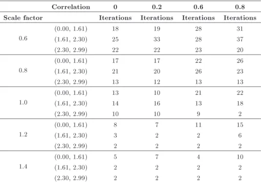
Table 6 represents the number of iterations in the column generation method, according to the dif-ferent correlation measures inside the nests. It shows that changing the correlation measure between each nest's products will alter the buy up and no-purchase probability. The algorithm tries to balance these eects and this leads to an increasing or decreas-ing number of iterations. It can be observed that, generally, when there is ample capacity in the high scale factor and high no-purchase utility, increasing correlation will lead to simplifying oer set structures. In order to explain the causes of this eect, consider a case in which the scale factor is 1, and the no-purchase observed utility is (2.3,2.99). If we solve this problem, the optimum solution will be degenerated with three oer sets. Results are summarized in Table 7.
These results should be analyzed based on the fact that products 19 and 20 are low fare products and belong to the same nest. Figure 3 shows the trend of dierent sets oering time periods according to the product correlations of the nest.
When the product correlation of the nests is zero, removing products 19 and 20 will lead to an increase in other product choice probabilities, with the same rate. But, increasing correlation will result in the choice probability of product 12 (low fare product) to be increased more than other high fare products, and this leads to reductions in buy up probability
Table 6. Number of iterations in the column generation algorithm.
Correlation 0 0.2 0.6 0.8
Scale factor Iterations Iterations Iterations Iterations 0.6
(0.00, 1.61) 18 19 28 31
(1.61, 2.30) 25 33 28 37
(2.30, 2.99) 22 22 23 20
0.8
(0.00, 1.61) 17 17 22 26
(1.61, 2.30) 21 20 26 23
(2.30, 2.99) 13 12 13 13
1.0
(0.00, 1.61) 13 10 21 22
(1.61, 2.30) 14 16 13 18
(2.30, 2.99) 10 10 9 2
1.2
(0.00, 1.61) 8 7 11 15
(1.61, 2.30) 3 2 2 6
(2.30, 2.99) 2 2 2 2
1.4
(0.00, 1.61) 5 7 4 10
(1.61, 2.30) 2 2 2 2
(2.30, 2.99) 2 2 2 2
Table 7. Oer sets and their optimal oering period.
Correlation 0 0.2 0.6 0.8 Oer set 1 (1, 2, 3, 4, 5, 6, 7, 8, 9, 10, 11, 12, 13, 14, 15, 16, 17, 18, 19, 20, 21, 22) 572 604 947 1000 Oer set 2 (1, 2, 3, 4, 5, 6, 7, 8, 9, 10, 11, 12, 13, 14, 15, 16, 17, 18, 20, 21, 22) 224 208 39 0 Oer set 3 (1, 2, 3, 4, 5, 6, 7, 8, 9, 10, 11, 12, 13, 14, 15, 16, 17, 18, 20, 21, 22) 204 288 14 0
Figure 3. Optimal oering period of dierent sets.
and increases departure with no-purchase probability. Then, as seen in Figure 3, increasing correlation will result in a decrease in the oering time period of sets 2 and 3. But, when we decrease capacity, buy up will become more important than departure with no-purchase, and then we will not observe the mentioned behavior.
Computational results show that in 88% of cases, a heuristic without the Boltzmann operator and genetic
Figure 4. Path of the best and mean of population in dierent generations.
algorithm manages to nd the entering column and, then, the heuristic works well itself.
Figure 4 represents the path of the best and mean of populations in dierent generations in a genetic algorithm with parameters = 0:6. The
no-purchase utility is (1.61,2.30) and the nest correlation is 0.8.
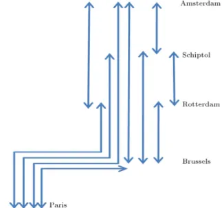
5.2. Railroad network
A specic railroad network in Europe is used by Hosseinalifam [23] for a test problem, a part of which we will consider with ve cities and four legs. There are two high (H) and low (L) fare classes on each leg. Figure 5 illustrates this railroad network.
In this problem, there are 10 trains with a capac-ity of 100 passengers going from Paris to Amsterdam. Each train stops in Brussels, Rotterdam, Schiptol and Amsterdam. Thus, there are 10 markets shown in Table 8. Two fare classes and 10 markets produce a total of 60 products.
Customers are divided into 20 dierent segments based on their sensitivity to prices, their origin and ultimate destination and 40 nests. Table 9 shows each segment's denition according to our assumptions. We assume that the booking horizon includes 2000 time periods and each segment includes two nests. The
Figure 5. Railroad network.
Table 8. Products denition in railroad network. O-D Low fare High fare
PAR-BRU 200 400
PAR-RTA 300 500
PAR-SCH 350 525
PAR-AMA 350 525
BRU-RTA 150 250
BRU-SCH 175 275
BRU-AMA 200 300
RTA-SCH 50 100
RTA-AMA 175 300
SCH-AMA 50 100
experiments are done for three scale factors, including 0.5, 1 and 1.5 for time periods.
Table 10 represents a 95% condence interval for the improvement percent, while the rm changes the choice model from a multinomial to a nested logit model.
The rst column in this table is the case in which correlations in all nests are zero. As we expect, all condence intervals in this condition include zero and both model outputs are the same.
Following the previous network, scarce capacity leads to an increase in the importance of choosing the correct choice model for oering the most suitable products for customers, and ample capacity decreases this sensitivity.
6. Conclusion
This article focuses on the eects of specic choice models on network revenue management. Most re-search focusing on choice-based revenue management, usually applies a multinomial logit choice model. In spite of the simplicity of this model, it has some serious limitations, such as the independence of irrel-evant alternatives. We explained this restriction and compared it with the multinomial logit choice model in this article. In order to overcome this restriction, we introduce the nested logit model, the most well known model after multinomial logit. One of the challenges faced by scientists in revenue management is incorporation of more realistic choice models in traditional models without signicantly increasing the complexity of the problem. One of the most applicable models of based revenue management is choice-based deterministic linear programming. Considering the exponential number of variables in this problem, a column generation technique is used for solving it. The subproblem of this algorithm is sensitive to the specic choice model used in the original problem. We changed the choice model and introduced the new subproblem structure. By referring to previous studies, we showed that the new subproblem is Np-hard and a heuristic algorithm is required for solving it in real conditions. A combination of heuristic and metaheuristic algorithms is proposed for solving the new subproblem. The heuristic algorithm assures that we can reach a reasonable point and the metaheuristic would improve it if the previous algorithm stopped at a local optimum point. The simulation study was done under two dierent conditions. We assume that the real choice model customers use for specifying a product is nested logit, and we analyze the eects of using the multinomial logit model by the rm to determine the oer sets. The results show that when there is scarce capacity, specifying an accurate choice model is very important and can improve organization revenue.
Table 9. Customer segmentation in railroad network problem. Segment O-D Nest Consideration
set
Preference vector
No-purchase utility
Arrival rate
1 PAR-BRU 1 1, 2, 3 10, 55, 25 8 0.08
2 4, 5, 6 20, 4, 3 8 0.08
2 PAR-BRU 1 1, 2, 3 8, 38, 18 60 0.02
2 4, 5, 6 60, 10, 7 60 0.02
3 PAR-RTA 1 7, 8, 9 15, 30, 20 2 0.08
2 10, 11, 12 8, 2, 1 2 0.08
4 PAR-RTA 1 7, 8, 9 10, 25, 8 45 0.02
2 10, 11, 12 25, 10, 4 45 0.02
5 PAR-SCH 1 13, 14, 15 25, 25, 20 10 0.08
2 16, 17, 18 2, 2, 2 10 0.08
6 PAR-SCH 1 13, 14, 15 10, 12, 15 30 0.02
2 16, 17, 18 21, 3, 3 30 0.02
7 PAR-AMA 1 19, 20, 21 20, 20, 2 4 0.08
2 22, 23, 24 3, 4, 3 4 0.08
8 PAR-AMA 1 19, 20, 21 8, 5, 2 35 0.02
2 22, 23, 24 20, 3, 3 35 0.02
9 BRU-RTA 1 25, 26, 27 10, 60, 50 15 0.08
2 28, 29, 30 4, 3, 2 15 0.08
10 BRU-RTA 1 25, 26, 27 4, 25, 20 70 0.02
2 28, 29, 30 45, 4, 6 70 0.02
11 BRU-SCH 1 31, 32, 33 5, 25, 10 5 0.08
2 34, 35, 36 4, 3, 3 5 0.08
12 BRU-SCH 1 31, 32, 33 2, 14, 3 40 0.02
2 34, 35, 36 7, 6, 4 40 0.02
13 BRU-AMA 1 37, 38, 39 30, 24, 4 6 0.08
2 40, 41, 42 2, 2, 2 6 0.08
14 BRU-AMA 1 37, 38, 39 25, 12, 2 10 0.02
2 40, 41, 42 6, 5, 4 10 0.02
15 RTA-SCH 1 43, 44, 45 10, 25, 20 4 0.08
2 46, 47, 48 4, 3, 2 4 0.08
16 RTA-SCH 1 43, 44, 45 3, 13, 12 30 0.02
2 46, 47, 48 36, 3, 2 30 0.02
17 PAR-AMA 1 49, 50, 51 20, 40, 10 5 0.08
2 52, 53, 54 2, 1, 2 5 0.08
18 PAR-AMA 1 49, 50, 51 10, 15, 5 40 0.02
2 52, 53, 54 25, 25, 3 40 0.02
19 SCA-AMA 1 55, 56, 57 30, 32, 20 5 0.08
2 58, 59, 60 4, 3, 2 5 0.08
20 SCA-AMA 1 55, 56, 57 20, 24, 15 60 0.02
2 58, 59, 60 20, 4, 4 60 0.02
Table 10. Condence interval for the improvement percent while rm switches to the NL model. Correlation
0 0.2 0.4 0.6 0.8
Time periods C.I. C.I. C.I. C.I. C.I.
1000 (-0.672,0.924) (-0.309,1.097) (-0.969,0.356) (-1.044,0.590) (0.840,2.147) 2000 (-0.678,0.241) (-0.009,0.984) (0.499,1.406) (2.556,3.495) (6.353,7.584) 3000 (-0.542,0.386) (-0.344,0.550) (0.258,1.112) (3.096,4.110) (8.299,9.500)
Improvement percent condence intervals indicate that even if statistical tests demonstrate a correlation be-tween unobserved parts of utility functions, it is not benecial under all conditions to change the choice model in the optimization module immediately and increase the complexity of calculations. We studied the relationship between correlation measure and rm revenue under dierent conditions, and analyzed the number of iterations, with respect to the correlation measure in dierent nests. We also showed that changing the correlation will lead to a change in buy up and no-purchase probability. The algorithm tries to balance these eects, which causes a change in the number of iterations of the column generation algorithm.
For future work, the nested logit model could be applied to other choice-based revenue management algorithms. Further work can be done to prove, analytically, the improvement in changing specic choice models. Finally, research can be planned to incorporate other realistic choice models and analyze their eects in the choice-based revenue management models.
References
1. Talluri, K.T. and Van Ryzin, G., The Theory and Practice of Revenue Management, New York, Kluwer Academic Publishers (2004).
2. Belobaba, P. and Hopperstad, C. \Boeing/MIT sim-ulation study: PODS results update", In AGIFORS Reservation and Yield Management Study Group Sym-posium Proceedings, London (1999).
3. Anderson, S. \Passenger choice analysis for seat capac-ity control: A pilot project in Scandinavian airlines", International Transactions in Operational Research, 5(6), pp. 471-486 (1998).
4. Algers, S. and Beser, M. \Modelling choice of ight and booking class-a study using stated preference and revealed preference data", International Journal of Services Technology and Management, 2(1), pp. 28-45 (2001).
5. Zhang, D. and Cooper, W.L. \Revenue management for parallel ights with customer-choice behavior", Operations Research, 53(3), pp. 415-431 (2005).
6. Van Ryzin, G. and Vulcano, G. \Computing virtual nesting controls for network revenue management under customer choice behavior", Manufacturing & Service Operations Management, 10(3), pp. 448-467 (2008).
7. Chen, L. and Homem-de-Mello, T. \Mathematical programming models for revenue management under customer choice", European Journal of Operational Research, 203(2), pp. 294-305 (2010).
8. Talluri, K. and Van Ryzin, G. \Revenue management under a general discrete choice model of consumer behavior", Management Science, 50, pp. 15-33 (2004).
9. Gallego, G. et al. \Managing exible products on a network", department of industrial engineering and operations research, Columbia University (2004).
10. Liu, Q. and Van Ryzin, G. \On the choice-based lin-ear programming model for network revenue manage-ment", Journal of Manufacturing & Service Operations Management, 10, pp. 288-311 (2008).
11. Bront, J.J.M., Mendez-Daz, I. and Vulcano, G. \A column generation algorithm for choice-based network revenue management", Operations Research, 57(3), pp. 769-784 (2009).
12. Kunnumkal, S. and Topaloglu, H. \A rened de-terministic linear program for the network revenue management problem with customer choice behavior", Naval Research Logistics (NRL), 55(6), pp. 563-580 (2008).
13. Vulcano, G., Van Ryzin, G. and Chaar, W. \Choice-based revenue management: An emprical study of es-timation and optimization", Manufacturing & Service Operations Management, 12, pp. 371-392 (2010).
14. Amaruchkul, K. and Sae-Lim, P. \Airline overbooking models with misspecication", Journal of Air Trans-port Management, 17, pp. 143-147 (2011).
15. Meissner, J. and Strauss, A. \Improved bid prices for choice-based network revenue management", European Journal of Operational Research, 217, pp. 417-427 (2012).
16. Derigs, U. and Friederichs, S. \On the application of a transportation model for revenue optimization in waste management: a case study", Central European Journal of Operations Research, 17, pp. 81-93 (2008).
17. Schutze, J. \Pricing strategies for perishable products: the case of Vienna and the hotel reservation systems hrs.com", Central European Journal of Operations Research, 16, pp. 43-66 (2008).
18. Ben-Akiva, M.E. and Lerman, S.R., Discrete Choice Analysis: Theory and Application to Travel Demand, 9, The MIT Press (1985).
19. Train, K.E., Discrete Choice Methods with Simulation, New York, Cambridge University Press (2009).
20. Garrow, L.A., Discrete Choice Modelling and Air Travel Demand, Georgia Institute of Technology, USA: Ashgate Publishing Company (2010).
21. Prokopyev, O.A., Huang, H.X. and Pardalos, P.M. \On complexity of unconstrained hyperbolic 0-1 pro-gramming problems", Operations Research Letters, 33(3), pp. 312-318 (2005).
Systems, The University of Michigan Press, Ann Arbor (1975).
23. Hosseinalifam, M., A Fractional Proframming Ap-proach for Choice-Based Network Revenue Manage-ment, Montreal University (2009).
Biographies
Farhad Etebari is PhD candidate in the Industrial Engineering Department of K.N. Toosi University of Technology. His research interests include optimization models, choice-based revenue management, transporta-tion planning, AI algorithms and logistic systems. He has several publications in these elds.
Abdollah Aghaei is a professor in the Industrial
Engineering Department of K.N. Toosi University of Technology. His research interests include model-ing and computer simulation, knowledge management and technology, project management and e-marketing. Professor Aaghaie has authored several books and technical publications in archival journals.
Ammar Jalalimanesh is a faculty member of Ira-nian Research Institute for Information Science and Technology. He is PhD student in the Industrial Engineering and Management System Department of Amirkabir University of Technology. He holds a master degree in Industrial Engineering from K.N. Toosi University of Technology. His research interests include AI algorithms and modeling of complex sys-tems.