Comparison of Prediction Methods for Air Pollution Data in Malaysia and Singapore

Comparison of Prediction Methods for Air Pollution

Data in Malaysia and Singapore

Merlinda Wibowo

UTM Big Data Centre, Ibnu Sina Institute for Scientific and Industrial Research, Faculty of Computing, Universiti Teknologi Malaysia, UTM Johor Bahru, Johor,

Malaysia

[email protected]

Sarina Sulaiman, Siti Mariyam Shamsuddin

Industrial Research, Faculty of Computing, Universiti Teknologi Malaysia, UTM Johor Bahru, Johor,

Malaysia [email protected]

Submitted: 04/04/2018. Revised edition: 15/06/2018. Accepted: 26/06/2018. Published online: 21 November 2018

Abstract—The process for analyzing and extracting useful information from a large database that employs one or more machine learning techniques is Data Mining. There are many data mining methods that can be used in a variety of data patterns. One of them is prediction modeling. This study compares several data mining performance methods for prediction such as Naïve Bayes, Random Tree, J48, and Rough Set to get the most powerful classifier to extract the knowledge of air pollution data. The parameters being used for observation in the performance of the prediction methods are correctly and incorrectly classified instances, the time taken, and kappa statistic. The experimental result reveals that Rough Set is extremely good for classifying the Air Pollutant Index (API) data from Malaysia and Singapore. Rough Set has the lowest error and the highest performance compared to other methods with the accuracy more than 97%.

Keywords—Data mining; prediction method; air pollutant index; naïve bayes; random tree; J48; Rough Set

I. INTRODUCTION

The level of air quality is getting lower due to the high level of air pollution, especially in urban area. The decrease of air quality level is also caused by many factors, like the number of vehicles, the number of factories and industrial development, land fires, stacking of garbage, natural disaster, and others [1]. It is necessary to measure and classify air quality every day. The measurement and classification results of air quality greatly assist the government in making a policy. This policy aims to control air pollution to achieve the best air quality standard for human and animal survival. Documentation of this results can be stored in a database with large scale because the data will increase to a large number.

With the development of information technology, it should be able to help find the hidden information knowledge in data with statistical and mathematical calculation methods [2]. This information later can be used as a policy that is more accurate, fast and efficient. In addition, information technology can also help spreading the information to the public that can access it anywhere and anytime in real time. Data mining can provide predictive capabilities for policy decision-making processes to predict precautions and alter the outcome of process that happened before [3]. Extraction of the model describes the importance of data classes and predict future of the data trends by using classification and also prediction. This method is also expected to optimize data management processes.

This study discusses several data mining methods and compares the performance of the methods for prediction such as Naïve Bayes, J48, Random Tree, and Rough Set to get the powerful classifier to extract the knowledge of air pollution data. Experiment and the result of this study will also be described in this paper followed by the conclusion and future work.

II. AIR POLLUTION DATA

pollution is caused by the human activity itself. The principle of air pollution occurs in the air when there is a pollutant element that comes from natural activity and also from the human activities. Air pollution can affect the balance of air quality and disruption for the survival of humans and animals [4].

Air pollution leads to several diseases and estimated 3 million deaths per year due to allergic conjunctivitis, allergic rhinitis, asthma, stroke, heart disease, lung cancer, and chronic respiratory disease [5][6][7]. Ambient air pollution affects developed, developing, low and middle-income countries, but the largest number of burden is Western Pacific and Southeast Asia regions [5]. People living in urban areas have air quality level higher than other areas. Quality monitor of ambient air data is used to assess exposure estimation in air pollution. Many places have established monitoring network with historical especially in urban areas.

Forest fire in Indonesia affects the terrible haze to Malaysia and Singapore in 2015. This forest fire is caused by El Niño storm that makes extreme weather condition. El Nino storm can raise the ocean temperature. Rainy season delayed and drought all over the country, affects the water supply, and many others [8]. This conditions happened again in early 2016 and even worse.

Air Pollutant Index (API) is a standard value of air pollution levels developed by The Environmental Protection Agency (USEPA). Malaysian Air Quality Guidelines (MAAGs) is the basic standard of the API in Malaysia that has been adapted to the recommendations of WHO [9]. While there is a special institution to deal with issues related to smoke in Singapore, including early warning of fog, measurement, and dissemination of air quality information that is National Environment Agency (NEA). According to USEPA, the standard value of API will be divided into several levels that are [9]:

 Good. It means low pollution levels and it does not give a bad effect on human health at all. This level is indicated by a value less than 50.

 Moderate. This level does not give adverse effect to human health. It is indicated by value 51 to 100.

 Unhealthy. This level means that air pollution can aggrieve human health conditions especially those who have lung complications. It is indicated by value 101 to 200.

 Very Unhealthy. It means air pollution can affect human health and little tolerance for people with heart and lung complications to do physical exercise. This level is indicated by value 201 to 300.

 Hazardous. This level is indicated by value more than 300. This air pollution is very risky and also very dangerous to human health.

The API value is calculated by all parameter. The kind of air pollution parameters are Nitrogen Dioxide (NO2), Sulfur Dioxide (sO2), Carbon Monoxide (CO), Particulate Matter

(PM10), and Ozone (O3) [4]. This API value is obtained for each air quality parameters. The final value of API is taken from the highest API value of calculation air quality result from all parameters. The API is viewed as the gold standard of government reference for characterizing and determining ambient air quality but the data is still limited by space and time [1]. The prediction of API value for air pollution can provide valuable information and enhance the scientific understanding about ambient air quality in Malaysia and Singapore. This ability can also provide a better understanding for the observed level of API to give the useful, accurate, fast, and effective information.

III. PREDICTION METHODS

Data mining is a process to analyze and extract useful information of a large database that employs one or more machine learning techniques [3]. Data mining is different from data warehouse. Data mining is a field that fully uses what the data warehouse produces [3], [10]. Data warehouse is assigned to query data from the raw database to provide data that can be used to handle management, reporting, and data mining. Then this data mining will extract the new information from the data provided by the data warehouse. There are many data mining methods that can be used in a variety of data patterns. One of them is prediction modeling. These methods will be used to answer the question regarding the obscurity. This methods will perform hypothesis validation, querying and reporting, multidimensional analysis, online analytic processing, and statistical analysis.

This study applies data mining by comparing four methods to find the most influential factor and to find the most accurate algorithm to utilize air pollution data that can be a useful information by rules generated. The following methods used for prediction modeling are:

A. Naïve Bayes

Naive Bayes method uses probability and statistical knowledge by applying Bayes' theorem. This classification method has been described in previous research [11][12]. The Bayes Theorem is described as [13]:

Here, the parameter c indicates the class variable, F = (f1, f2,... fn) arise for the object and the feature molecular descriptors (variables) of an object is represented by the (f1, f2,..., fn). P(c) is the main or minor probability that is fixed for all classes, P(c|F) and P(F|c) show the rear probability. In the classification, all molecular descriptors (attribute) releases the value of the class variable, such as:

Naive Bayes is the simplest form of Bayesian Network Classifier. Each node in Naive Bayes has a node feature class as a parent but does not have a parent other features node [14][15]. Based on the fact Naïve Bayes is a method for classification [16]. This method can be divided into five main categories. They are structure extension, feature selection, feature weighting, local learning, and instance weighting [13].

The relationship between Naïve Bayes and classification, hypothesis correlation, and classification evidence is the hypotheses in Bayes' theorem which are targeted classified labels by mapping in classification, whereas evidence is the features to input into the classification model [10]. From previous research shows that Naïve Bayes has to use all the attributes contained in the data. Then, each of which will be analyzed to show the importance and independence of every attribute [17]. A large number of study show that such a surprisingly simple naive classifier Bayesian can be competitive with state-of-the-art classifiers. By utilizing this method, several studies conducted based on weights of evidence [18][19][20][21][17]. There are many model approaches proposed to improve Naïve Bayes [12][13].

B. Decision Tree (J48)

J48 is an algorithm that is used to construct the decision trees and the modification result from C4.5 and ID3 algorithm [22]. This method is an open source java implementation in data mining tool that creates binary tree as part of C4.5 decision tree. J48 is simple C4.5 decision trees for prediction of the Decision Tree. Decision Tree is a useful approach in predicting problem [23][24][25]. J48 used the concept from information entropy. The entropy (E) is given by following Equation (4) in which pP; pN are the proportion of positive, negative (training) examples.

J48 ignores the missing values while building a tree. The item value based on what is known by the attribute values can be predicted for other records [23]. The basic idea from this algorithm is to divide data into range for the item that is found in the training sample based on attribute values and allow classification via either decision trees or rules generated [24]. The J48 algorithm can be seen in Fig. 1.

Fig. 1. J48 Algorithm [23]

There are several previous researches that have been done by using this method. By using WEKA Tools, gradient images can be analyzed to recognize the individuality of characters [26], to implement the character detection system with an artificial neural network [27], to analyze the object with the histogram group calculated for all the pieces of a script and compare the distance between two different scripts with WEKA [28], and to calculate the typefaces with the geometrical arrangement to present a simple and quick approach for author detection [24][25].

J48 is experimented using various settings to train and obtain acceptable model accuracy. This method is simple to understand and interpret, which means people are able to understand this methods after a brief explanation. Among other data mining methods, J48 requires little data preparation and able to handle both numerical and categorical data [23].

C. Random Tree

Random Tree learns about a decision tree but only use a random subset of attributes for each split from available attributes. Random Tree is basic algorithm of the decision tree that collaborates with Quinlan C4.5 or Classification and Regression Trees (CART) to select random attribute before it is implemented with subset size that is determined by the part ratio parameter. This algorithm can build a decision tree using a portion of the data for training data and select the feature to cut the value that maximizes the gain of the information [29]. Random Tree is strong and easy to implement, produce highly accurate predictions.

Representation of data as a tree has advantages over other approaches. Data becomes more meaningful and easy to interpret. It can create a classification model that predicts the value of the label based on some input from the dataset sample attribute.

There are two stages of building Random Tree as follows:

result structure or called a tree skeleton will repeat until the tree achieves the specified depth [30].

2)Training data used to specify the appropriate value or classifications.

This method that can combine the large sets of random trees generally leads to accurate model. Random trees are generated efficiently, computed and scored for multiple tree skeletons. For example, combining the different trees into an ensemble as usual can make prediction done. There has been an extensive research in the recent years in the field of Machine Learning with Random Trees approach. Fig. 2 shows the training process of the random tree algorithm that is in the form of a simple summary.

Fig. 2. Random Tree Algorithm [29]

Random Tree consists of two stages. The first step generates the Build Tree Structure of each dataset. Since the leaves does not contain class distribution, statistics are referred to the skeleton. However, the skeleton building requires only information about the feature instead of training data. The second step is Update Statistics. In this step, to compute class statistic for the leaf nodes uses the training data.

Cutting is a technique where leaf nodes that do not increase the discriminatory power of the decision tree are removed. This is to change a tree more specific or more fitting for a more general form to increase the prediction power on the invisible dataset. Post-cutting is a type of parallel pruning done for the tree-making process after the previous tree-making is completed.

D. Rough Set

Rough Set is one of the mathematical technique to manage uncertainty, ambiguity and vagueness of Artificial Intelligence (AI) application. This method is efficient technique for Knowledge Discovery of Database (KDD) in data mining. In general, Rough Set defined as a theory attracts much attention of researchers and practitioners who contribute to the development of applications [31]. This method was initiated by

Pawlak in 1982 and can be claimed as similar to the Fuzzy Set Theory [32]. It can be used to find relationships in data and extract the knowledge from the data itself. This knowledge from extraction of dataset in the form of rule will easily be understood and meaningful.

Rough Set offers two element of data representation that is Information System (IS) and Decision System (DS). An information system is a set of object (U) and Conditional attribute (A) that is set of the example and condition attribute sequentially. In many applications, decision of classification is represented by a Decision Attribute (C). Decision system is a collection of dataset consists of m object and n attribute with the decision attribute therefore information system is (IS) = (U, {A, C}). In general, the important concept of Rough Set is Discerning Object, such as indiscernibility, equivalence class, discernibility matrix, and reduct [33][34].

1) Indiscerbinility Relation. A set of objects that have the same decision value DS = (U, {A, C}).

2) Equivalence Class. Grouping the same objects for attributes A (U, A).

3) Discernibility Matrix. Discernibility is a central point of Rough Set Theory. It uncovers a fact that says knowledge is not enough to discern multiple objects by using existing information [35]. The discernibility matrix is generated when discernibility function can be defined. The discernibility function is a Boolean function (true or false) that constructed for each object.

4) Reduct is selecting attributes from a set of attribute conditions using prime implicant with boolean function. A collection of all prime implicants determines sets of reduct.It can simplify the functions and minimize the solution. Rules will be generated from reduct are representative rule extracted from the dataset. Since a reduct is not unique, rule sets generated from different reduct contain different sets of rules.

According to previous research, Rough Set is contrast to other techniques because main part of Rough Set can identify with minimal subset of conditional attribute that has properties which is similar discernible complete attribute set [35][36]. Rough Set has been used in many application such as medicine, banking, decision analysis, image processing, and pharmacology. Rough Set has also been successfully applied in various fields, such as decision-making, data mining, machine learning, and pattern acknowledge [2][34].

IV. EXPERIMENTAL SETUP

Fig. 3. Schema of Analytic Process for Air Pollutant Index (API) Dataset

The proposed scheme developed from a previous scheme [38]. The basic steps from this schema are data collection, pre- data processing and data extraction, pattern discovery, and validation and interpretation. The input of this study is API dataset and the output is the value of classification accuracy result and training error result.

A. Data Collection

This study uses two datasets, Air Pollutant Index (API) data from Malaysia and Singapore from 2014 until 2015. The data taken from Malaysian Government Open Data about API (http://data.gov.my/) and Singapore Government Pollutant Standard Index (http://www.haze.gov.sg/). The total of the dataset is 245,753 data. The API dataset contains dataset number, date, state, region, and API value in CSV format. The reading of API is a common and easiest method to describe the status of air quality. The API value and air pollution standard value is directly proportional, the higher API values indicates the higher values of air quality.

B. Data Pre-processing

Before mining process starts, there are three steps for pre-process data which are selection data, cleaning data, and transformation data. Selection data is selecting the set of data, creating the data target and focus on the sample data. The cleaning process includes removing duplication of data, checking inconsistent data, and fixing data errors (e.g. typographic errors). Moreover, data also needs enrichment or what is called transformation data. Data can be enriched with other relevant information. In this study, the API dataset enriches the decision attribute. Table I shows the API dataset from Malaysia and Singapore government open data.

TABLE I. THE SAMPLE OF API DATASET FOR MALAYSIA AND

SINGAPORE

No. Date Tim

e State Region API Decision

1 25/11

/2014 8:00 AM

Pulau

Pinang USM 51 Moderate

2 25/11

/2014 8:00 PM

Kelanta n

Tanah

Merah 18 Good

No. Date Tim

e State Region API Decision

3 25/11

/2014 8:00

PM Johor Muar 38 Good

4 25/11

/2014 8:00

PM North

Woodlan

d 47 Good

5 25/11

/2014 8:00

PM West Changi 46 Good

6 02/03

/2015 1:00 PM

Kelanta n

Tanah

Merah 67 Moderate

… … … …

24575 3

02/04 /2015

11:0

0 PM Kedah

Bakar

Arang 54 Moderate

Pre-processed, analyzed, and transformed data represent air pollution data in appropriate format and useful for assisting the next process, data mining process.

C. Pattern Discovery

Data mining was used to analyze and extract knowledge automatically with one or many methods for air pollutant data to provide the useful, effective, and relevant information. It can show the areas that have a good condition or not. This information can also be used to predict the future air quality condition in all areas. There are four methods that were implemented in this study, which are Naïve Bayes, Random Tree, J48, and Rough Set. In order to investigate the dataset by using the tools this method is applied. WEKA is a tool for running the dataset. WEKA run the data for Naïve Bayes, Random Tree, J48, Rough Set algorithm. Evaluation selected of classifier is used 10-fold cross validation. It is also used based on the amount of data and suggested by WEKA.

D. Result and Discussion

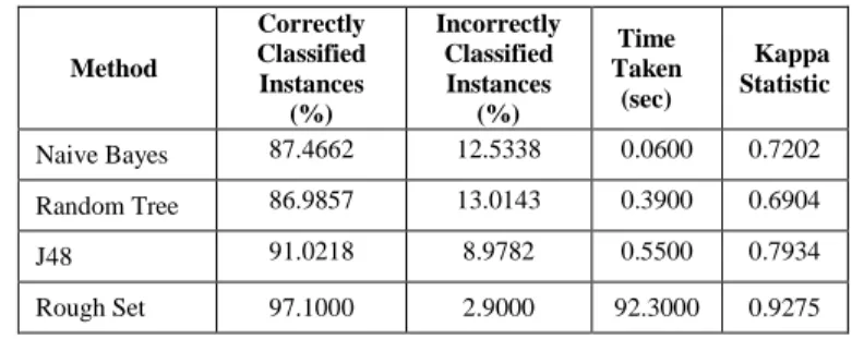
Evaluation phase is evaluating one or more performance of methods to get better quality and effectiveness method. It will help to choose the proper prediction method to investigate air pollution data for Malaysia and Singapore and also will be implemented in mobile analytic database summarization proposed work. In order to verify the performance of proposed methods, it used a statistical validation. The experiment results of this phase are shown in Table II and Table III. Table II shows the result based on correctly and incorrectly classified instances, the time taken, and kappa statistic.

TABLE II. CLASSIFICATION ACCURACY RESULT

Method

Correctly Classified Instances

(%)

Incorrectly Classified Instances

(%)

Time Taken

(sec)

Kappa Statistic

Naive Bayes 87.4662 12.5338 0.0600 0.7202

Random Tree 86.9857 13.0143 0.3900 0.6904

J48 91.0218 8.9782 0.5500 0.7934

From Table II and Fig. 4, we can see that Rough Set algorithm has the higher accuracy with 97.10% than other methods. But execution time of Rough Set is the slowest one. The fastest execution time is Naïve Bayes with 0.06 second. Even though Naïve Bayes has fastest time taken but the accuracy is lower than Rough Set. To evaluate the accuracy of any measurement that usually differentiate data collected reliability and validity, kappa statistic is used. The average of kappa statistic is 0.8-0.9, it shows substantial value. The visualization with graph of the accuracy methods depicted in Fig. 4.

Fig. 4. Visualization Methods Accuracy

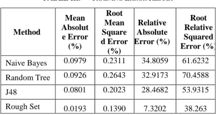
Table III shows the classification result based on error during execution process of testing data. In the Table III, we can see the mean absolute error, root mean squared error, relative absolute error, and root relative squared error. The lower error rate is more preferable. The method which has the lower error rate has powerful classification capability and ability.

TABLE III. TRAINING ERROR RESULT

Method

Mean Absolut e Error (%)

Root Mean Square d Error

(%)

Relative Absolute Error (%)

Root Relative Squared Error (%)

Naive Bayes 0.0979 0.2311 34.8059 61.6232

Random Tree 0.0926 0.2643 32.9173 70.4588

J48 0.0801 0.2023 28.4682 53.9315

Rough Set _{0.0193 0.1390 7.3202 38.263}

Based on the result of classifications that have been done, Rough Set has the highest accuracy compared to other methods but Rough Set has a lowest execution time. Rough Set can be the best method to analyze the air pollution data. This method can also generate the rules that is more efficient, relevant and accurate.

V. CONCLUSION AND FUTURE WORK

This study has been successfully to compare the performance of different data mining methods, which are Naïve Bayes, Random Tree, J48, and Rough Set. These methods can classify the Air Pollutant Index (API) from Malaysia and Singapore datasets. It can help to extract the knowledge of data, to predict the future of the data, and possible to make the right decision concerning safety and health of the population. The best performance classification is Rough Set that has the highest accuracy but has the lowest error.

In the future work, we will combine the selected method to other proper methods that can maximize the data processing with a large amount of data. It will give better results, faster execution time, more accurate, and more effective.

ACKNOWLEDGMENT

This study supported by Ministry of Higher Education Malaysia (MOHE), Ministry of Science, Technology and Innovation Malaysia (MOSTI) and Universiti Teknologi Malaysia (UTM). This paper is financially supported by E-Science Fund, R.J130000.7928.4S117, PRGS Grant,

R.J130000.7828.4L680, GUP Tier 1 UTM,

Q.J130000.2528.13H48, FRGS Grant, R.J130000.7828.4F634 and IDG Grant, R.J130000.7728.4J170. The Authors would like to express their deepest gratitude to the Research Management Centre (RMC), UTM for the support in research and development, Malaysian Administrative Modernisation and Planning Unit (MAMPU) for the shared Malaysia’s open government data and Soft Computing Research Group (SCRG) for the inspiration to make this study success.

REFERENCES

[1] J. Zhang and W. Ding. (2017). Prediction of Air Pollutants Concentration Based on an Extreme Learning Machine: The Case of Hong Kong. International Journal of Environmental

Research and Public Health, 14.

[2] M. Wibowo, S. Sulaiman, and S. M. Shamsuddin. (2017). Machine Learning in Data Lake for Combining Data Silos.

International Conference on Data Mining and Big Data,

10387, 294-306.

[3] K. Siwek and S. Osowski. (2016). Data Mining Methods for Prediction of Air Pollution, Int. J. Appl. Math. Comput. Sci., 26(2), 467-478.

[4] M. A. Bravo, M. Fuentes, Y. Zhang, M. J. Burr, and M. L. Bell. (2012). Comparison of Exposure Estimation, Methods for Air Pollutants: Ambient Monitoring Data and Regional Air Quality Simulation, Environ Res., 116, 1-10.

[5] WHO. (2016). Ambient Air Pollution: A Global Assessment of Exposure and Burden of Disease.

[7] A. Prus-Ustun, J. Wolf, C. Carvalan, R. Bos, and M. Neira. (2016). Preventing Disease Through Healthy Environment, WHO.

[8] World Bank. (2015). Indonesia’s Fire and Haze Crisis. Retrieved:

http://www.worldbank.org/en/news/feature/2015/12/01/indones ias-fire-and-haze-crisis.

[9] WHO. (2017). Evaluation of WHO air Quality Guidelines: Past, Present, and Future.

[10] E. Prasetyo. (2012). Data Mining, Andi.

[11] J. O. Berger. (2013). Statistical Decision Theory and Bayesian

Analysis. Springer Science and Bussiness Media.

[12] L. Jiang, C. Li, S. Wang, and L. Zhang. (2016). Deep Feature Weighting for Naïve Bayes and its Application to Text Classification, Eng. Appl. Artif. Intell., 52, 22-39.

[13] L. Jiang, D. Wang, and Z. Chai. (2012). Discriminatively Weighted Naïve Bayes and its Application in Text Classication,

Int. J. Artificical Intelligent Tools, 21 (1).

[14] J. R.. Quinlan, (1993). C4. 5: Programs for Machine Learning, Morgan Kaufmann, San Mateo.

[15] X. Wu, V. Kumar, J.R. Quinlan, J. Ghosh, and Q. Yang. (2008). Top 10 Algorithms in Data Mining, Knowl. Inf. Syst.,

14 (1), 1-37.

[16] E. H. Khalil. (2014). A Noise Tolerant Fine Tuning Algorithm for the Naive Bayesian Learning Algorithm, J. King Saud Univ.

– Comput. Inf. Sci., 26(2), 237-246.

[17] M. Kouli, C. Loupasakis, P. Soupios, D. Rozos, F. Vallianatos. (2014). Landslide Susceptibility Mapping by Comparing the WLC and WofE Multi-criteria Methods in the West Crete Island, Greece Environ, Earth Sci., 72(12), 5197-5219. [18] P. Tsangaratos and L. Ilia. (2016). Comparison of a Logistic

Regression and Naïve Bayes Classifier in Landslide Susceptibility Assessments: The Influence of Models Complexity and Training Dataset Size, Catena, 145, 164-179. [19] I. Ilia and P. Tsangaratos. (2015). Applying Weight of

Evidence Method and Sensitivity Analysis to Produce a Landslide Susceptibility Map, Landslides, 10.

[20] H. R. Pourghasemi, H. R. Moradi, and S. M. Fatemi Aghda. (2013). Landslide Susceptibility Mapping by Binary Logistic Regression, Analytical Hierarchy Process, and Statistical Index Models and Assessment of Their Performances, Nat. Hazards,

69(1), 749-779.

[21] H. R. Pourghasemi, A. G. Jirandeh, B. Pradhan, C. Xu, and C. Gokceoglu. (2013). Landslide Susceptibility Mapping Using Support Vector Machine and GIS at the Golestan Province,

Iran J. Earth Syst. Sci., 122(2), 349-369.

[22] A. K. Yadav and S. Chandel. (2014). Solar Radiation Prediction Using Artificial Neural Network Techniques: A Review Renewable and Sustainable. Energy Reviews, 33, 772-781.

[23] P. N. V. Kumar and V. R. Reddy. (2014). Novel Web Proxy Cache Replacement Algorithm using Machine Learning,

International Journal of Engineering Sciences and Research

Technology, 3(1), 339-346.

[24] T. R. Patil and S. S. Sherekar. (2013). Performance Analysis of Naïve Bayes and J48 Classification Algorithm for Data Classification, International Journal od Computer Science and

Applications, 6(2), 256-261.

[25] G. Suarez-Tangil, J. E. Tapiador, P. Peris-Lopez, and S.

Pastrana. (2015). Poweraware Anomaly Detection in

Smartphones: An Analysis of On-Platform Versus Externalized Operation, Persuasive and Mobile Computing, 18, 137-151. [26] C. Halder, K. Thakur, S. Phadikar, and K. Roy. (2015). Writer

Identification from Handwritten Devanagari Script, Information

Systems Design and Intelligent Systems and Computing, 340.

[27] S. Souza and J. M. Abe. (2014). Handwritten Numerical Characters Recognition Based on Paraconsistent Artificial Neural Networks, International Publishing Switzerland, 513, 93-102.

[28] W. M. Hannah, B. E. Mapes, and G. S. Elsaesser. (2016). A

Lagrangian View of Moisture Dynamics during DYNAMO, J.

Atmos. Sci., 73(5), 1967-1985.

[29] W. Fan, H. Wang, P. S. Yu, and S. Ma. (2003). Is Random Model Better? On its Accuracy and Efficiency, Proceeding 3rd

IEEE International Conference on Data Mining, 51-58.

[30] W. Gao, R. Grossman, Y. Gu, and P. S. Yu, (2009). Why Naïve

Ensembles Do Not Work in Cloud Computing, IEEE

International Computer Society, 282-289,.

[31] S. Rissino, and G. Lambert-Torres. (2009). Rough Set Theory– Fundamental Concepts, Principals, Data Extraction, and Applications, Data Min. Knowl. Discov. Real Life Appl. J. Ponce A. Karahoca (Eds.).

[32] Z. Pawlak. (1982). Rough Sets, Int. J. Comput. Inf. Sci., 11, 341-356.

[33] D. Srivastava, S. Bastra, and S. Bhalotia. (2015). Efficiant Rule Set Generation using K-Map & Rough Set Theory (RST),

International Journal of Engineering and Technology, 2 (3).

[34] M. Wibowo, S. Sulaiman, S. M. Shamsuddin, H. Hashim, and D. H. A. Ibrahim. (2017). Mobile Anlaytics Database Summarization Using Rough Set, International Journal of

Innovative Computing, 7(2), 6-12.

[35] M. N. A. Rahman, Y. M. Lazim, F. Mohamed, S. I. A. Saany and K. M. Yusof. (2013). Rules Generation for Multimedia Data Classifying using Rough Sets Theory, International

Journal of Hybrid Information Technology, 6 (5), 209-218.

[36] E. S. M. El-Alfy, and M. A. Alshammari. (2016). Towards Scalable Rough Set Based Attribute Subset Selection for Intrusion Detection Using Parallel Genetic Algorithm in MapReduce, Simul. Model. Pract. Theory, 1-12

[37] B. W. Fang, and B. Q. Hu, (2016). Probabilistic Graded Rough Set and Double Relative Quantitative Decision-Theoretic Rough Set, Int. J. Approx. Reason, 74, 1-12.

[38] N. B. Ahmad and S. M. Shamsuddin, (2010). A Comparative Analysis of Mining Techniques for Authomatic Detection of Student’s Learning Style, IEEE International Conference on