The science of computing

(1)

The science of computing

first edition

by Carl Burch

Copyright c 2004, by Carl Burch. This publication may be redistributed, in part or in whole, provided that this page is included. A complete version, and additional resources, are available on the Web at

(2)

(3)

3.1.4 Other bases . . . 17 3.2 Integer representation . . . 18 3.2.1 Unsigned representation . . . 18 3.2.2 Sign-magnitude representation . . . 18 3.2.3 Two’s-complement representation . . . 19 3.3 General numbers . . . 21 3.3.1 Fixed-point representation . . . 22 3.3.2 Floating-point representation . . . 22 3.4 Representing multimedia . . . 27

3.4.1 Images: The PNM format . . . 27

3.4.2 Run-length encoding . . . 28

3.4.3 General compression concepts . . . 29

3.4.4 Video . . . 30

3.4.5 Sound . . . 30

4 Computational circuits 33 4.1 Integer addition . . . 33

(4)

4.2.1 Latches . . . 35

4.2.2 Flip-flops . . . 38

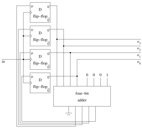
4.2.3 Putting it together: A counter . . . 39

4.3 Sequential circuit design (optional) . . . 40

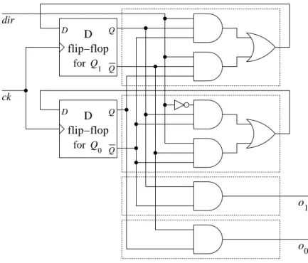
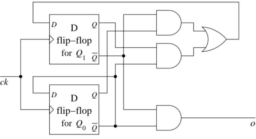
4.3.1 An example . . . 40 4.3.2 Another example . . . 42 5 Computer architecture 45 5.1 Machine design . . . 45 5.1.1 Overview . . . 45 5.1.2 Instruction set . . . 46

5.1.3 The fetch-execute cycle . . . 48

5.1.4 A simple program . . . 48

5.2 Machine language features . . . 49

5.2.1 Input and output . . . 49

5.2.2 Loops . . . 50

5.3 Assembly language . . . 51

5.3.1 Instruction mnemonics . . . 51

5.3.2 Labels . . . 52

5.3.3 Pseudo-operations . . . 52

5.4 Designing assembly programs . . . 53

5.4.1 Pseudocode definition . . . 53

5.4.2 Pseudocode examples . . . 55

5.4.3 Systematic pseudocode . . . 56

5.5 Features of real computers (optional) . . . 57

5.5.1 Size . . . 57

5.5.2 Accessing memory . . . 58

5.5.3 Computed jumps . . . 58

6 The operating system 61 6.1 Disk technology . . . 61

6.2 Operating system definition . . . 62

6.2.1 Virtual machines . . . 62 6.2.2 Benefits . . . 63 6.3 Processes . . . 64 6.3.1 Context switching . . . 64 6.3.2 CPU allocation . . . 66 6.3.3 Memory allocation . . . 68 7 Artificial intelligence 71 7.1 Playing games . . . 71

7.1.1 Game tree search . . . 72

7.1.2 Heuristics . . . 73

7.1.3 Alpha-beta search . . . 74

7.1.4 Summary . . . 74

7.2 Nature of intelligence . . . 74

7.2.1 Turing test . . . 74

(5)

CONTENTS iii

7.2.3 Symbolic versus connectionist AI . . . 76

7.3 Neural networks . . . 77

7.3.1 Perceptrons . . . 77

7.3.2 Networks . . . 78

7.3.3 Computational power . . . 79

7.3.4 Case study: TD-Gammon . . . 79

8 Language and computation 81 8.1 Defining language . . . 81 8.2 Context-free languages . . . 82 8.2.1 Grammars . . . 82 8.2.2 Context-free languages . . . 83 8.2.3 Practical languages . . . 84 8.3 Regular languages . . . 86 8.3.1 Regular expressions . . . 86 8.3.2 Regular languages . . . 88

8.3.3 Relationship to context-free languages . . . 88

9 Computational models 91 9.1 Finite automata . . . 91 9.1.1 Relationship to languages . . . 93 9.1.2 Limitations . . . 93 9.1.3 Applications . . . 94 9.2 Turing machines . . . 95 9.2.1 Definition . . . 95 9.2.2 An example . . . 96 9.2.3 Another example . . . 98 9.2.4 Church-Turing thesis . . . 100 9.3 Extent of computability . . . 101 9.3.1 Halting problem . . . 102

9.3.2 Turing machine impossibility . . . 103

10 Conclusion 107

(6)

(7)

Chapter 1

Introduction

Computer science is the study of algorithms for transforming information. In this course, we explore a

variety of approaches to one of the most fundamental questions of computer science: What can computers do?

That is, by the course’s end, you should have a greater understanding of what computers can and cannot do. We frequently use the term computational power to refer to the range of computation a device can accomplish. Don’t let the word power here mislead you: We’re not interested in large, expensive, fast equipment. We want to understand the extent of what computers can accomplish, whatever their efficiency. Along the same vein, we would say that a pogo stick is more powerful than a truck: Although a pogo stick may be slow and cheap, one can use it to reach areas that a large truck cannot reach, such as the end of a narrow trail. Since a pogo stick can go more places, we would say that it is more powerful than a truck. When applied to computers, we would say that a simple computer can do everything that a supercomputer can, and so it is just as powerful.

1.1 Common misconceptions about computer science

Most students arrive to college without a good understanding of computer science. Often, these students choose to study computer science based on their misconceptions of the subject. In the worst cases, students continue for several semesters before they realize that they have no interest in computer science. Before we continue, let me point out some of the most common misconceptions.

Computer science is not primarily about applying computer technology to business needs. Many colleges have such a major called “Management Information Systems,” closely related to a Management or Business major. Computer science, on the other hand, tends to take a scientist’s view: We are interested in studying computation in itself. When we do study business applications of computers, the concentration is on the techniques underlying the software. Learning how to use the software effectively in practice receives much less emphasis.

Computer science is not primarily about building faster, better computers. Many colleges have such a major called “Computer Engineering,” closely related to an Electrical Engineering major. Although com-puter science entails some study of comcom-puter hardware, it focuses more on comcom-puter software design, theo-retical limits of computation, and human and social factors of computers.

(8)

Computer science is not primarily about writing computer programs. Computer science students learn how to write computer programs early in the curriculum, but the emphasis is not present in the “real” computer science courses later in the curriculum. These more advanced courses often depend on the un-derstanding built up by learning how to program, but they rarely strive primarily to build programming expertise.

Computer science does not prepare students for jobs. That is, a good computer science curriculum isn’t designed with any particular career in mind. Often, however, businesses look for graduates who have studied computer science extensively in college, because students of the discipline often develop skills and ways of thinking that work well for these jobs. Usually, these businesses want people who can work with others to understand how to use computer technology more effectively. Although this often involves programming computers, it also often does not.

Thinking about your future career is important, but people often concentrate too much on the quantifiable characteristics of hiring probabilities and salary. More important, however, is whether the career resonates with your interests: If you can’t see yourself taking a job where a major in is important, then majoring in isn’t going to prove very useful to your career, and it may even be a detriment. Of course, many students choose to major in computer science because of their curiosity, without regard to future careers.

1.2 Textbook goals

This textbook fulfills two major goals.

It satisfies the curiosity of students interested in an overview of practical and theoretical approaches to the study of computation.

Students who believe they may want to study computer science more intensively can get an overview of the subject to help with their discernment. In addition to students interested in majoring or minoring in computer science, these students include those who major in something else (frequently the natural sciences or mathematics) and simply want to understand computer science well also.

The course on which this textbook is based (CSCI 150 at the College of Saint Benedict and Saint John’s University) has three major units, of roughly equal size.

Students learn the fundamentals of how today’s electronic computers work (Chapters 2 through 6 of this book). We follow a “bottom-up” approach, beginning with simple circuits and building up toward writing programs for a computer in assembly language.

Students learn the basics of computer programming, using the specific programming language of Java (represented by the Java Supplement to this book).

Students study different approaches to exploring the extent of computational power (Chapters 7 to 10 of this book).

(9)

Chapter 2

Logic circuits

We begin our exploration by considering the question of how a computer works. Answering this question will take several chapters. At the most basic level, a computer is an electrical circuit. In this chapter, we’ll examine a system that computer designers use for designing circuits, called a logic circuit.

2.1 Understanding circuits

2.1.1 Logic circuits

A logic circuit consists of lines, representing wires, and peculiar shapes called logic gates. There are three types of logic gates:

NOT gate AND gate OR gate

The relationship of the symbols to their names can be difficult to remember. I find it handy to remember that the word AND contains a D, and this is what an AND gate looks like. We’ll see how logic gates work in a moment.

Each wire carries a single information element, called a bit. A bit’s value can be either 0 or 1. In electrical terms, you can think of zero volts representing 0 and five volts representing 1. (In practice, there are many systems for representing 0 and 1 with different voltage levels. For our purposes, the details of voltage are not important.) The word bit, incidentally, comes from Binary digIT; the term binary comes from the two (hence bi-) possible values.

Here is a diagram of one example logic circuit.

out x

y

We’ll think of a bit travelling down a wire until it hits a gate. You can see that some wires intersect in a small, solid circle: This circle indicates that the wires are connected, and so values coming into the circle

(10)

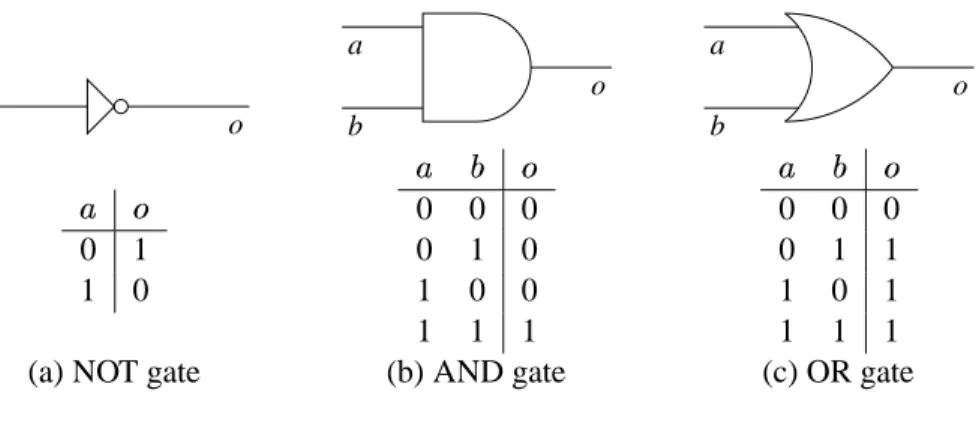
a o a b o a b o 0 1 1 0 0 0 0 0 1 0 1 0 0 1 1 1 0 0 0 0 1 1 1 0 1 1 1 1

(a) NOT gate (b) AND gate (c) OR gate

Figure 2.1: Logic gate behavior.

continue down all the wires connected to the circle. If two wires intersect with no circle, this means that one wire goes over the other, like an Interstate overpass, and a value on one wire has no influence on the other.

Suppose that we take our example circuit and send a 0 bit on the upper input ( ) and a 1 bit on the lower

input ( ). Then these inputs would travel down the wires until they hit a gate.

0 1 x y out 1 1 0 0

To understand what happens when a value reaches a gate, we need to define how the three gate types work.

NOT gate: Takes a single bit and produces the opposite bit (Figure 2.1(a)). In our example circuit, since

the upper NOT gate takes 0 as an input, it will produce 1 as an output.

AND gate: Takes two inputs and outputs 1 only if both the first input and the second input are 1

(Fig-ure 2.1(b)). In our example circuit, since both inputs to the upper AND gate are 1, the AND gate will output a 1.

OR gate: Takes two inputs and outputs 1 if either the first input or the second input are 1 (or if both are 1)

(Figure 2.1(c)).

After the values filter through the gates based on the behaviors of Figure 2.1, the values in the circuit will be as follows. 0 1 1 0 1 x y out 1 1 1 1 0 0 0 0

(11)

2.2 Designing circuits 5

Based on this diagram, we can see that when is 0 and is 1, the output

is 1.

By doing the same sort of propagation for other combinations of input values, we can build up a table of how this circuit works for different combinations of inputs. We would end up with the following results.

0 0 0 0 1 1 1 0 1 1 1 0

Such a table, representing what a circuit computes for each combination of possible inputs, is a truth table. The second row, which says that

is 1 if is 0 and is 1, corresponds to the propagation illustrated

above.

2.1.2 Practical considerations

Logic gates are physical devices, built using transistors. At the heart of the computer is the central

process-ing unit (CPU), which includes millions of transistors.

The designers of the CPU worry about two factors in their circuits: space and speed. The space factor relates to the fact that each transistor takes up space, and the chip containing the transistors is limited in size, so the number of transistors that fit onto a chip is limited by current technology. Since CPU designers want to fit many features onto the chip, they try to build their circuits with as few transistors as possible to accomplish the tasks needed. To reduce the number of transistors, they try to create circuits with few logic gates.

The second factor, speed, relates to the fact that transistors take time to operate. Since the designers want the CPU to work as quickly as possible, they work to minimize the circuit depth, which is the maximum distance from any input through the circuit to an output. Consider, for example, the two dotted lines in the following circuit, which indicate two different paths from an input to an output in the circuit.

x y

The dotted path starting at goes through three gates (an OR gate, then a NOT gate, then another OR gate),

while the dotted path starting at goes through only two gates (an AND gate and an OR gate). There are

two other paths, too, but none of the paths go through more than three gates. Thus, we would say that this circuit’s depth is 3, and this is a rough measure of the circuit’s efficiency: Computing an output with this circuit takes about three times the amount of time it takes a single gate to do its work.

2.2 Designing circuits

In the previous section, we saw how logic circuits work. This is helpful when you want to understand the behavior of a circuit diagram. But computer designers face the opposite problem: Given a desired behavior, how can we build a circuit with that behavior? In this section, we look at a systematic technique for designing circuits. First, though, we’ll take a necessary detour through the study of Boolean expressions.

(12)

2.2.1 Boolean algebra

Boolean algebra, a system of logic designed by George Boole in the middle of the nineteenth century, forms

the foundation for modern computers. George Boole noticed that logical functions could be built from AND, OR, and NOT gates and that this observation leads one to be able to reason about logic in a mathematical system.

As Boole was working in the nineteenth century, of course, he wasn’t thinking about logic circuits. He was examining the field of logic, created for thinking about the validity of philosophical arguments. Philosophers have thought about this subject since the time of Aristotle. Logicians formalized some common mistakes, such as the temptation to conclude that if implies , and if holds, then must hold also.

(“Brilliant people wear glasses, and I wear glasses, so I must be brilliant.”)

As a mathematician, Boole sought a way to encode sentences like this into algebraic expressions, and he invented what we now call Boolean expressions. An example of a Boolean expression is “ .” A

line over a variable (or a larger expression) represents a NOT; for example, the expression corresponds to

feeding through a NOT gate. Multiplication (as with ) represents AND. After all, Boole reasoned, the

AND truth table (Figure 2.1(b)) is identical to a multiplication table over 0 and 1. Addition (as with )

represents OR. The OR truth table (Figure 2.1(c)) doesn’t match an addition table over 0 and 1 exactly — although 1 plus 1 is 2, the result of 1 OR 1 is 1 — but, Boole decided, it’s close enough to be a worthwhile analogy.

In Boolean expressions, we observe the regular order of operations: Multiplication (AND) comes before addition (OR). Thus, when we write , we mean . We can use parentheses when this order

of operations isn’t what we want. For NOT, the bar over the expression indicates the extent of the expression to which it applies; thus, represents NOT OR , while representsNOT ORNOT.

A warning: Students new to Boolean expressions frequently try to abbreviate as — that is, drawing

a single line over the whole expresion, rather than two separate lines over the two individual pieces. This abbreviation is wrong. The first, , translates to NOT ANDNOT (that is, both and are 0), while translates to NOT AND (that is, and aren’t both 1). We could draw a truth table comparing the

results for these two expressions.

0 0 1 1 1 0 1

0 1 1 0 0 0 1

1 0 0 1 0 0 1

1 1 0 0 0 1 0

Since the fifth column ( ) and the seventh column ( ) aren’t identical, the two expressions aren’t

equiva-lent.

Every expression directly corresponds to a circuit and vice versa. To determine the expression cor-responding to a logic circuit, we feed expressions through the circuit just as values propagate through it. Suppose we do this for our circuit of Section 2.1.

y x y x y x y x y x out + y x y x

The upper AND gate’s inputs are and , and so it outputs . The lower AND gate outputs , and the

(13)

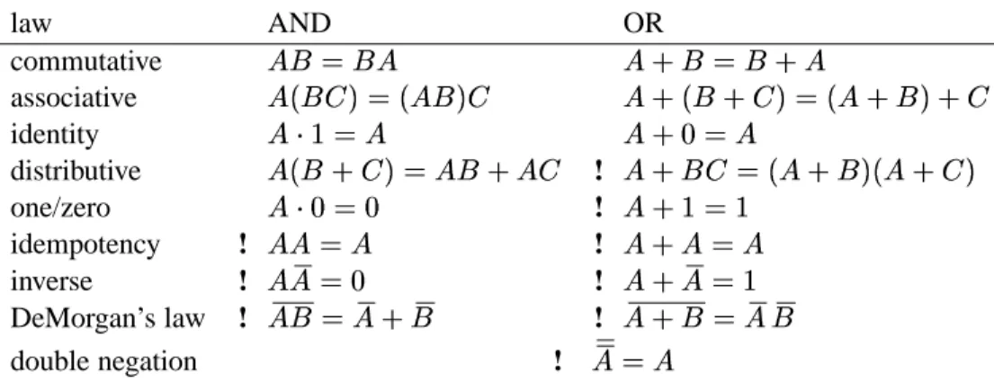
2.2 Designing circuits 7 law AND OR commutative associative identity distributive ! one/zero ! idempotency ! ! inverse ! ! DeMorgan’s law ! ! double negation !

Figure 2.2: A sampler of important laws in Boolean algebra.

2.2.2 Algebraic laws

Boole’s system for writing down logical expressions is called an algebra because we can manipulate symbols using laws similar to those of algebra. For example, the commutative law applies to both OR and AND. To prove that OR is commutative (that is, that

), we can complete a truth table demonstrating

that for each possible combination of and , the values of and are identical.

0 0 0 0

0 1 1 1

1 0 1 1

1 1 1 1

Since the third and fourth columns match, we would conclude that

is a universal law.

Since OR (and AND) are commutative, we can freely reorder terms without changing the meaning of the expression. The commutative law of OR would allow us to transform into , and the

commutative law of AND (applied twice) allows us to transform to .

Similarly, both OR and AND have an associative law (that is,

). Because of this associativity, we won’t bother writing parentheses across the same operator when we write Boolean expressions. In drawing circuits, we’ll freely draw AND and OR gates that have several inputs. A 3-input AND gate would actually correspond to two 2-input AND gates when the circuit is actually wired. There are two possible ways to wire this.

A + (B + C) A B C A B C _A B C (A + B) + C

Because of the associative law for AND, it doesn’t matter which we choose.

There are many such laws, summarized in Figure 2.2. This includes analogues to all of the important algebraic laws dealing with multiplication and addition. There are also many laws that don’t hold with addition and multiplication; these are marked with an exclamation point in the table.

(14)

2.2.3 Converting a truth table

Now we can return to our problem: If we have a particular logical function we want to compute, how can we build a circuit to compute it? We’ll begin with a description of the logical function as a truth table. Suppose we start with the following function for which we want a circuit.

0 0 0 0 0 0 1 1 0 1 0 1 0 1 1 0 1 0 0 0 1 0 1 0 1 1 0 1 1 1 1 1

Given such a truth table defining a function, we’ll build up a Boolean expression representing the func-tion. For each row of the table where the desired output is 1, we describe it as the AND of several factors.

description 0 0 1 1 0 1 0 1 1 1 0 1 1 1 1 1

To arrive at a row’s description, we choose for each variable either that variable or its negation, depending on which of these is 1 in that row. Then we take the AND of these choices. For example, if we consider the first of the rows above, we consider that since is 0 in this row, is 1; since is 0, is 1; and is 1. Thus,

our description is the AND of these choices, . This expression gives 1 for the combination of values

on this row; but for other rows, its value is 0, since every other row is different in some variable, and that variable’s contribution to the AND would yield 0.

Once we have the descriptions for all rows where the desired output is 1, we observe the following: The value of the desired circuit should be 1 if the inputs correspond to the first 1-row, the second 1-row, the third 1-row, or the fourth 1-row. Thus, we’ll combine the expressions describing the rows with an OR.

Note that we do not include rows where the desired output is 0 — for these rows, we want none of the AND terms to yield 1, so that the OR of all terms gives 0.

The expression we get is called a sum of products expression. It is called this because it is the OR (a sum, if we understand OR to be like addition) of several ANDs (products, since AND corresponds to multiplication). We call this technique of building an expression from a truth table the sum of products

technique.

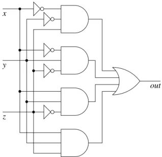
This expression leads immediately to the circuit of Figure 2.3. In general, this technique allows us take any function over bits and build a circuit to compute that function. The existence of such a technique proves that circuits can compute any logical function.

Note, incidentally, that the depth of this circuit will always be three (or less), since every path from input to output will go through a NOT gate (maybe), an AND gate, and an OR gate. Thus, this technique shows that it’s never necessary to design a circuit that is more than three gates deep. Sometimes, though, designers build deeper circuits because they are concerned not only with speed, but also with size: A larger circuit can often accomplish the same task using fewer gates.

(15)

2.3 Simplifying circuits 9

out y

x

z

Figure 2.3: A circuit derived from a given truth table.

2.3 Simplifying circuits

The circuit generated by the sum-of-products technique can be quite large. This is impractical: Additional gates cost money, so CPU designers want to use gates as economically as possible to make room for more features or to reduce costs. Thus, we’d like to make a smaller circuit accomplishing the same thing, if possible.

We can simplify a circuit by taking the corresponding expression and reducing it using laws of Boolean algebra. We will insert this simplification step into our derivation process. Thus, our approach for converting a truth table into a circuit will now have three steps.

1. Build a sum of products expression from the truth table.

2. Simplify the expression using laws of Boolean algebra (as in Figure 2.2). 3. Draw the circuit corresponding to this simplified expression.

In the rest of this section, we look at a particular technique for simplifying a Boolean expression. Our technique for simplifying expressions works only for sum-of-products expressions — that is, the expression must be an OR of terms, each term being an AND of variables or their negations.

Suppose we want to simplify the expression

1. We look through the terms looking for all pairs that are identical in every way, except for one variable that is NOTted in one and not NOTted in the other. Our example has two such pairs.

and differ only in . and differ only in .

(16)

2. We create a new expression. This expression includes a single term for each pair from step 1; this term keeps everything that the pair shares in common. The expression also keeps any terms that do not participate in any pairs from step 1. For our example, this would lead us to the following.

The term arises because this term does not belong to a pair from step 1; we include due to the pair, in which and are the common factors; and we include due to the

pair. Note that we include a term for every pair, even if some pairs overlap (that is, if two pairs include the same term).

The following reasoning underlies this transformation.

Using the law that

, we can duplicate the term, which appears in two of the

pairs.

Because of the associative and commutative laws of OR, we can rearrange and insert parentheses so that the pairs are together.

We’ll concentrate on the first pair ( ) in the following. (The reasoning for the other

pair, , proceeds similarly.)

has two terms with in common. Using the distributive law of AND over OR, we

get .

We can apply the law

to get .

Finally, we apply AND’s identity law (

) to get .

3. If there are duplicates among the terms, we can remove the duplicates. This is justified by the Boolean algebra law that

. (There are no duplicates in this case.)

4. Return to step 1 to see if there are any pairs in this new expression. (In our working example, there are no more pairs to be found.)

Thus, we end up with the simplified expression

From this we can derive the smaller circuit of Figure 2.4 that works the same as that of Figure 2.3. In this case we have replaced the 10 gates of Figure 2.3 with only 7 in Figure 2.4.

(17)

2.3 Simplifying circuits 11

x

z

out y

(18)

(19)

Chapter 3

Data representation

Since computer science is the study of algorithms for transforming information, an important element of the discipline is understanding techniques for representing information. In this chapter, we’ll examine some techniques for representing letters, integers, real numbers, and multimedia.

3.1 Binary representation

One of the first problems we need to confront is how wires can represent many values, if a wire can only carry a 0 or 1 based on its electrical voltage.

3.1.1 Combining bits

A wire can carry one bit, which can represent up to two values. But suppose we have several values. For example, suppose we want to remember the color of a traffic light (red, amber, or green). What can we do?

We can’t do this using a single wire, since a wire carries a single bit, which can represent only two values (0 and 1). Thus, we will need to add more bits. Suppose we use two wires. Then we can assign colors to different combinations of bits on the two wires.

wire 1 wire 2 meaning

0 0 red

0 1 amber

1 0 green

For example, if wire 1 carries 0 and wire 2 carries 1, then this would indicate that the light is amber. In fact, with two bits we can represent up to four values: The fourth combination, , was unnecessary for the traffic light.

If we want to represent one of the traditional colors of the rainbow (red, orange, yellow, green, blue, indigo, violet), then two bits would not be enough. But three bits would be: With three bits, there are four distinct values where the first bit is 0 (since there are four different combinations for the other two bits) and four distinct values where the first bit is 1, for a total of eight combinations, which is enough for the rainbow’s seven colors.

In general, if we have bits, we can represent distinct values through various combinations of the

bits’ values. In fact, this fact is so important that, to emphasize it, we will look at a formal proof.

(20)

Proof: For each bit, we have two choices, 0 or 1. We make the choices independently, so we can

simply multiply the number of choices for each bit.

times

There are, therefore, different combinations of choices.

Computers often deal with English text, so it would be nice to have some way of assigning distinct values to represent each possible printable character on the keyboard. (We consider lower-case and capital letters as different characters.) How many bits do we need to represent the keyboard characters?

If you count the symbols on the keyboard, you’ll find that there are 94 printable characters. Six bits don’t provide enough distinct values, since they provide only

different combinations, but seven is plenty (

). Thus, we can represent each of the 94 possible printable characters using seven bits. Of

course, seven bits actually permit up to 128 different values; the extra 34 can be dedicated to the space key, the enter key, the tab key, and other convenient characters.

Many computers today use ASCII (American Standard Code for Information Interchange) for reprent-ing characters. This seven-bit codreprent-ing defines the space as 0100000, the capital A as 1000001, the zero digit as 0110000, and so on. Figure 3.1 contains a complete table of the ASCII codes. (Most of the extra 34 values, largely obscure abbrevations in the first column of Figure 3.1, are rarely used today.)

Computers deal with characters often enough that designers organize computer data around the size of their representation. Computer designers prefer powers of two, however. (This preference derives from the fact that bits can represent up to different values.) Thus, they don’t like dividing memory up into

units of seven bits (as required for the ASCII code). Instead, they break memory into groups of eight bits (

), each of which they call a byte. The extra bit is left unused when representing characters using

ASCII.

When they want to talk about large numbers of bytes, computer designers group them into kilobytes (KB). The prefixes kilo- come from the metric prefix for a thousand (as in kilometer and kilogram) However, because computers deal in binary, it’s more convenient to deal with powers of 2, and so the prefix kilo- in kilobyte actually stands for the closest power of 2 to 1000, which is

. These abbreviations extend upward. kilobyte KB 1,024 bytes megabyte MB 1,048,576 bytes gigabyte GB 1.074 billion bytes terabyte TB 1.100 trillion bytes 3.1.2 Representing numbers

We can already represent integers from zero to one using a single bit. To represent larger numbers, we need to use combinations of bits. The most convenient technique for assigning values to combinations is based on binary notation (also called base 2).

You’re already familiar with decimal notation (also called base 10). You may remember the following sort of diagram from grade school.

1 0 2 4

That is, in representing the number 1024, we put a 4 in the ones place, a 2 in the tens place, a 0 in the hundreds places, and a 1 in the thousands place. This system is called base 10 because there are 10 possible

Sometimes, manufacturers use powers of 10 instead of 2 for marketing purposes. Thus, they may advertise a hard disk as holding 40 GB, when it actually holds only 37.3 GB, or 40 billion bytes.

(21)

3.1 Binary representation 15 0 0000000 NUL 32 0100000 SP 64 1000000 @ 96 1100000 ‘ 1 0000001 SOH 33 0100001 ! 65 1000001 A 97 1100001 a 2 0000010 STX 34 0100010 " 66 1000010 B 98 1100010 b 3 0000011 ETX 35 0100011 # 67 1000011 C 99 1100011 c 4 0000100 EOT 36 0100100 $ 68 1000100 D 100 1100100 d 5 0000101 ENQ 37 0100101 % 69 1000101 E 101 1100101 e 6 0000110 ACK 38 0100110 & 70 1000110 F 102 1100110 f 7 0000111 BEL 39 0100111 ’ 71 1000111 G 103 1100111 g 8 0001000 BS 40 0101000 ( 72 1001000 H 104 1101000 h 9 0001001 HT 41 0101001 ) 73 1001001 I 105 1101001 i 10 0001010 NL 42 0101010 * 74 1001010 J 106 1101010 j 11 0001011 VT 43 0101011 + 75 1001011 K 107 1101011 k 12 0001100 NP 44 0101100 , 76 1001100 L 108 1101100 l 13 0001101 CR 45 0101101 - 77 1001101 M 109 1101101 m 14 0001110 SO 46 0101110 . 78 1001110 N 110 1101110 n 15 1001111 SI 47 0101111 / 79 1001111 O 111 1101111 o 16 0010000 DLE 48 0110000 0 80 1010000 P 112 1110000 p 17 0010001 DC1 49 0110001 1 81 1010001 Q 113 1110001 q 18 0010010 DC2 50 0110010 2 82 1010010 R 114 1110010 r 19 0010011 DC3 51 0110011 3 83 1010011 S 115 1110011 s 20 0010100 DC4 52 0110100 4 84 1010100 T 116 1110100 t 21 0010101 NAK 53 0110101 5 85 1010101 U 117 1110101 u 22 0010110 SYN 54 0110110 6 86 1010110 V 118 1110110 v 23 0010111 ETB 55 0110111 7 87 1010111 W 119 1110111 w 24 0011000 CAN 56 0111000 8 88 1011000 X 120 1111000 x 25 0011001 EM 57 0111001 9 89 1011001 Y 121 1111001 y 26 0011010 SUB 58 0111010 : 90 1011010 Z 122 1111010 z 27 0011011 ESC 59 0111011 ; 91 1011011 [ 123 1111011 { 28 0011100 FS 60 0111100 < 92 1011100 \ 124 1111100 | 29 0011101 GS 61 0111101 = 93 1011101 ] 125 1111101 } 30 0011110 RS 62 0111110 > 94 1011110 ˆ 126 1111110 ˜ 31 0011111 US 63 0111111 ? 95 1011111 _ 127 1111111 DEL

(22)

digits for each place (0 through 9) and because the place values go up by factors of 10 ( ).

In binary notation, we have only two digits (0 and 1) and the place values go up by factors of 2. So we have a ones place, a twos place, a fours place, an eights place, a sixteens place, and so on. The following diagrams a number written in binary notation.

1 0 1 1 This value, 1011

, represents a number with 1 eight, 0 fours, 1 two, and 1 one:

11 . (The parenthesized subscripts indicate whether the number is in binary notation or decimal notation.)

We’ll often want to convert numbers between their binary and decimal representations. We saw how to convert binary to decimal with 1011

. Here’s another example: Suppose we want to identify what 100100

represents. We first determine what places the 1’s occupy. 1 0 0 1 0 0

We then add up the values of these places to get a base-10 value:

36

.

To convert a number from decimal to binary, we repeatedly determine the largest power of two that fits into the number and subtract it, until we reach zero. The binary representation has a 1 bit in each place whose value we subtracted. Suppose, as an example, we want to convert 88

to binary. We observe the largest power of 2 less than 88 is 64, so we decide that the binary expansion of 88 has a 1 in the 64’s place, and we subtract 64 to get

. Then we see than the largest power of 2 less than 24 is 16, so we decide to put a 1 in the 16’s place and subtract 16 from 24 to get 8. Now 8 is the largest power of 2 that fits into 8, so we put a 1 in the 8’s place and subtract to get 0. Once we reach 0, we write down which places we filled with 1’s. 1 1 1

We put a zero in each empty place and conclude that the binary representation of 88

is 1011000

.

3.1.3 Alternative conversion algorithms

In the previous section, we saw a procedure (an algorithm) for converting between binary notation and dec-imal notation, and we saw another procedure for converting between decdec-imal notation and binary notation. Those algorithms work well, but there are alternative algorithms for each that some people prefer.

From binary To convert a number written in binary notation to decimal notation, we begin by thinking “0,” and we go through the binary representation left-to-right, each time adding that bit to twice the number we are thinking. Suppose, for example, that we want to convert 1011000

into decimal notation.

2 = + 2 = + 2 = + 2 = + 2 = + 2 = + 2 = + 1 0 1 1 0 0 0 (2) 1 0 1 1 0 0 0 44 88 22 11 5 2 1 0 1 2 5 11 22 44 (10)

(23)

3.1 Binary representation 17

We end up with the answer 88

.

This algorithm is based on the following reasoning. A five-bit binary number 10110

corresponds to

. This latter expression is equivalent to the polynomial

where , , , , , and

. We can convert this polynomial into an alternative

form.

In the algorithm, we’re computing based on the alternative form instead of the original polynomial.

To binary To convert a number in the opposite direction, we repeatedly divide a number by 2 until we reach 0, each time taking note of the remainder. When we string the remainders in reverse order, we get the binary representation of the original number. For example, suppose we want to convert 88

into binary notation. 2 2 2 2 2 2 2 88 44 22 11 5 2 1 0 R 0 R 0 R 0 R 0 R 1 R 1 R 1 1 0 1 1 0 0 0 (10) (2)

After going through the repeated division and reading off the remainders, we arrive at 1011000

.

Understanding how this process works is simply a matter of observing that it reverses the double-and-add algorithm we just saw for converting from binary to decimal.

3.1.4 Other bases

Binary notation, which tends to lead to very long numerical representations, is cumbersome for humans to remember and type. But using decimal notation obscures the relationship to the individual bits. Thus, when the identity of the individual bits is important, computer scientists often compromise by using a power of two as the base: The popular alternatives are base eight (octal) and base sixteen (hexadecimal).

The nice thing about these bases is how easily they translate into binary. Suppose we want to convert 173

to binary. One possible way is to convert this number to base 10 and then convert that answer to binary. But doing a direct conversion turns out to be much simpler: Since each octal digit corresponds to a three-bit binary sequence, we can replace each octal digit of 173

with its three-bit sequence. 1 7 3 001 111 011 Thus, we conclude 173 001111011 .

To convert the other way, we split the binary number we want to convert into groups of three (starting from the 1’s place), and then we replace each three-bit sequence with its corresponding octal digit. Suppose we want to convert 1011101 to octal. 1 0 1 1 1 0 1 1 3 5

The first known description of this is in 1299 by a well-known Chinese mathematician Chu Shih-Chieh (1270?–1330?). An obscure Englishman, William George Horner (1786–1837), later rediscovered the principle known today as Horner’s method.

(24)

Thus, we conclude 1011101 135 .

Hexademical, frequently called hex for short, works the same way, except that we use groups of four bits instead. One slight complication is that hexadecimal requires 16 different digits, and we have only 10 available. Computer scientists use Latin letters to fill the gap. Thus, after 0 through 9 come A through F.

0 0 0000 4 4 0100 8 8 1000 C 12 1100

1 1 0001 5 5 0101 9 9 1001 D 13 1101

2 2 0010 6 6 0110 A 10 1010 E 14 1110

3 3 0011 7 7 0111 B 11 1011 F 15 1111

As an example of a conversion from hex to decimal, suppose we want to convert the number F5

to base 10. We would replace the F with 1111

and the 5 with 0101

, giving its binary equivalent 11110101

.

3.2 Integer representation

We can now examine how computers remember integers on the computer. (Recall that integers are numbers with no fractional part, like , , or .)

3.2.1 Unsigned representation

Modern computers usually represent numbers in a fixed amount of space. For example, we might decide that each byte represents a number. A byte, however, is very limiting: The largest number we can fit is 11111111

255

, and we often want to deal with larger numbers than that.

Thus, computers tend to use groups of bytes called words. Different computers have different word sizes. Very simple machines have 16-bit words; today, most machines use 32-bit words, though some computers use 64-bit words. (The term word comes from the fact that four bytes (32 bits) is equivalent to four ASCII characters, and four letters is the length of many useful English words.) Thirty-two bits is plenty for most numbers, as it allows us to represent any integer from 0 up to

4,294,967,295. But the limitation is becoming increasingly irritating, and so people are beginning to move to 64-bit computers. (This isn’t because people are dealing with larger numbers today than earlier, so much as the fact that memory has become much cheaper, and so it seems silly to continue trying to save money by skimping on bits.)

The representation of an integer using binary representation in a fixed number of bits is called an

un-signed representation. The term comes from the fact that the only numbers representable in the system

have no negative sign.

But what about negative integers? After all, there are some perfectly respectable numbers below 0. We’ll examine two techniques for representing integers both negative and positive: sign-magnitude representation and two’s-complement representation.

3.2.2 Sign-magnitude representation

Sign-magnitude representation is the more intuitive technique. Here, we let the first bit indicate whether

the number is positive or negative (the number’s sign), and the rest tells how far the number is from 0 (its magnitude). Suppose we are working with 8-bit sign-magnitude numbers.

would be represented as 00000011 would be represented as 10000011

(25)

3.2 Integer representation 19

For 3

, we use 1 for the first bit, because the number is negative, and then we place into the remaining

seven bits.

What’s the range of integers we can represent with an 8-bit sign-magnitude representation? For the largest number, we’d want 0 for the sign bit and 1 everywhere else, giving us 01111111, or 127

. For the smallest number, we’d want 1 for the sign bit and 1 everywhere else, giving us 127

. An 8-bit sign-magnitude representation, then, can represent any integer from 127

to 127

.

This range of integers includes 255 values. But we’ve seen that 8 bits can represent up to 256 different values. The discrepency arises from the fact that the representation includes two representations of the number zero ( and , represented as 00000000 and 10000000).

Arithmetic using sign-magnitude representation is somewhat more complicated than we might hope. When you want to see if two numbers are equal, you would need additional circuitry so that is understood

as equal to . Adding two numbers requires circuitry to handle the cases of when the numbers’ signs

match and when they don’t match. Because of these complications, sign-magnitude representation is not often used for representing integers. We’ll see it again, however, when we get to floating-point numbers in Section 3.3.2.

3.2.3 Two’s-complement representation

Nearly all computers today use the two’s-complement representation for integers. In the two’s-complement system, the topmost bit’s value is the negation of its meaning in an unsigned system. For example, in an 8-bit unsigned system, the topmost bit is the 128’s place.

In an 8-bit two’s-complement system, then, we negate the meaning of the topmost bit to be instead.

To represent the number 100

, we would first choose a 1 for the ’s place, leaving us with

. (We are using the repeated subtraction algorithm described in Section 3.1.2. Since

the place value is negative, we subtract a negative number.) Then we’d choose a for the 16’s place, the 8’s

place, and the 4’s place to reach 0.

1 0 0 1 1 1 0 0

Thus, the 8-bit two’s-complement representation of 100

would be 10011100.

would be represented as 00000011 would be represented as 11111101

What’s the range of numbers representable in an 8-bit two’s-complement representation? To arrive at the largest number, we’d want 0 for the ’s bit and 1 everywhere else, giving us 01111111, or 127

. For the smallest number, we’d want 1 for the ’s bit and 0 everywhere else, giving 128

. In an 8-bit two’s-complement representation, we can represent any integer from 128

up to 127

. (This range includes 256 integers. There are no duplicates as with sig-magnitude representation.)

It’s instructive to map out the bit patterns (in order of their unsigned value) and their corresponding two’s-complement values.

(26)

bit pattern value 00000000 00000001 00000010 .. . 01111110 01111111 10000000 10000001 .. . 11111110 11111111

Notice that the two’s-complement representation wraps around: If you take the largest number, 01111111, and add 1 to it as if it were an unsigned number, and you get 10000000, the smallest number. This wrap-around behavior can lead to some interesting behavior. In one game I played as a child (back when 16-bit computers were popular), the score would go up progressively as you guided a monster through a maze. I wasn’t very good at the game, but my little brother mastered it enough that the score would hit its maximum value and then wrap around to a very negative value! Trying to get the largest possible score — without wrapping around — was an interesting challenge.

Negating two’s-complement numbers

For the sign-magnitude representation, it’s easy to represent the negation of a number: You just flip the sign bit. For the two’s-complement representation, however, the relationship between the representation of a number and the representation of its negation is not as obvious as one might like.

The following is a handy algorithm for relating the representation of a number to the representation of its negation: You start at the right, copying bits down, until you reach the first 1, beyond which you flip every bit. The representation of 12, for example, is 00001100, so its two’s complement representation will be 11110100 — the lower three bits (below and including the lowest 1) are identical, while the rest are all different. 0 0 0 0 1 1 0 0 1 0 0 1 1 1 1 0 -12 12 (10) (10)

last one bit bits to flip

Why this works is not immediately obvious. To understand it, we first need to observe that if we have a negative number and we interpret its two’s-complement representation in the unsigned format, we end

up with

. This is because the two’s-complement representation of will have a 1 in the uppermost

bit, representing , but when we interpret it as an unsigned number, we interpret this bit as representing , which is

more than before. The other bits’ values remain unchanged. Since the value of this uppermost bit has increased by

, the unsigned interpretation of the bit pattern is worth

more than the two’s-complement interpretation.

We can understand our negation algorithm as being a two-step process. 1. We flip all the bits (from 00001100 becomes 11110011, for example). 2. We add one to the number (which would give 11110100 in our example).

(27)

3.3 General numbers 21

Adding one to a number flips bits from the right, until we reach a zero. Since we already flipped all the bits in the first step, this second step flips these bits back to their original values.

Now we can observe that if the original number is when interpreted as an unsigned number, we will

have

after going through the process. The first step of flipping all bits is equivalent to subtracting

each bit from 1, which is the same as subtracting from the all-ones number ( ). Thus, after the first step,

we have the value . The second step adds one to this, giving us

. When

the unsigned representation of

is interpreted as a two’s-complement number, we understand it to be .

Adding two’s-complement numbers

One of the nice things about two’s-complement numbers is that you can add them just as you add regular numbers. Suppose we want to add and .

1001011 + 0011001

We can attempt to do this using regular addition, akin to the technique we traditionally use in adding base-10 numbers.

11111 1 11111101 + 00000101 100000010

We get an extra 1 in the ninth bit of the answer, but if we ignore this ninth bit, we get the correct answer. We can reason that this is correct as follows: Say one of the two numbers is negative and the other is positive. That is, one of the two numbers has a 1 in the ’s place, and the other has 0 there. If there is no

carry into the ’s place, then the answer is OK, because that means we got the correct sum in the last 7

bits, and then when we add the ’s place, we’ll maintain the represented by the 1 in that location

in the negative number.

If there is a carry into the ’s place, then this represents a carry of taken from summing the ’s

column. This carry of (represented by a carry of 1), added to the in that column for the negative

number (represented by a 1 in that column), should give us 0. This is exactly what we get we add the carry of 1 into the leftmost column to the 1 of the negative number in this column and then throw away the carry (

).

A similar sort of analysis will also work when we are adding two negative numbers or two positive numbers. Of course, the addition only works if you end up with something in the representable range. If you add 120 and 120 with 8-bit two’s-complement numbers, then the result of 240 won’t fit. The result of adding 120 and 120 as 8-bit numbers would turn out to be

!

For dealing with integers that can possibly be negative, computers generally use two’s-complement representation rather than sign-magnitude. It is somewhat less intuitive, but it allows simpler arithmetic. (It is true that negation is somewhat more complex, but only slightly so.) Moreover, the two’s-complement representation avoids the problem of multiple representations of the same number (0).

3.3 General numbers

Representing numbers as fixed-length integers has some notable limitations. It isn’t suitable for very large numbers that don’t fit into 32 bits, like

, nor can it handle numbers that have a fraction, like

. We’ll now turn to systems for handling a wider range of numbers.

(28)

3.3.1 Fixed-point representation

One possibility for handling numbers with fractional parts is to add bits after the decimal point: The first bit after the decimal point is the halves place, the next bit the quarters place, the next bit the eighths place, and so on.

Suppose that we want to represent 1.625

. We would want 1 in the ones place, leaving us with

.

Then we want 1 in the halves place, leaving us with

. No quarters will fit, so put a 0

there. We want a 1 in the eighths place, and we subtract from to get 0.

0 0 1 1 0 1

So the binary representation of

would be 1.101

.

The idea of fixed-point representation is to split the bits of the representation between the places to the left of the decimal point and places to the right of the decimal point. For example, a 32-bit fixed-point representation might allocate 24 bits for the integer part and 8 bits for the fractional part.

24 bits 8 bits

integer part fractional part To represent

, we would then write

The first three bytes give the , and the last byte gives the representation of

.

Fixed-point representation works well as long as you work with numbers within the given range. The 32-bit fixed-point representation described above can represent any multiple of

from 0 up to

16.7

million. But programs frequently need to work with numbers from a much broader range. For this reason, fixed-point representation isn’t used very often in today’s computing world.

3.3.2 Floating-point representation

Floating-point representation is an alternative technique based on scientific notation. Because we’re

work-ing with computers, we’ll base our scientific notation on powers of 2, not 10 as is traditional. For example, the binary representation of 5.5

is 101.1

. When we convert this to binary scientific notation, we move the decimal point to the left two places, giving us 1.011

. (This is just like converting 101.1

to scientific notation: It would be 1.011

.)

To represent a number written in scientific notation in bits, we’ll decide how to split up the representation to fit it into a fixed number of bits. First, let us define the two parts of scientific representation: In 1.011

, we call 1.011

the mantissa (or the significand), and we call the exponent. In this section we’ll

use 8 bits to store such a number, divided as follows.

exponent + 7 mantissa sign

1 bit 4 bits 3 bits

Financial software is a notable exception. Here, designers often want all computations to be precise to the penny, and in fact they should always be rounded to the nearest penny. There is no reason to deal with very large amounts (like trillions of dollars) or fractions of a penny. Such programs use a variant of fixed-point representation that represents each amount as an integer multiple of

(29)

We use the first bit to represent the sign (1 for negative, 0 for positive), the next four bits for the sum of 7 and the actual exponent (we add 7 to allow for negative exponents), and the last three bits for the fraction of the mantissa. Note that we omit the digit to the left of the decimal point: Since the mantissa has only one nonzero bit to the left of the decimal point, and the only nonzero bit is 1, we know that the bit to the left of the decimal point must be a 1. There’s no point in wasting space in inserting this 1 into our bit pattern. We include only the bits of the mantissa to the right of the decimal point.

We call this a floating-point representation because the values of the mantissa bits “float” along with the decimal point, based on the exponent’s given value. This is in contrast to fixed-point representation, where the decimal point is always in the same place among the bits given.

Continuing our example of 5.5 1.011 , we add 7 to 2 to arrive at 9 1001 for the exponent bits. Into the mantissa bits we place the bits following the decimal point of the scientific notation,

. This gives us

as the 8-bit floating-point representation of 5.5

. Suppose we want to represent 96

.

1. First we convert our desired number to binary: 1100000

. 2. Then we convert this to binary scientific notation: 1.100000

. 3. Then we fit this into the bits.

(a) We choose 1 for the sign bit if the number is negative. (It is, in this case.)

(b) We add 7 to the exponent and place the result into the four exponent bits. (In this case, we arrive at 13 1101 .)

(c) The three mantissa bits are the first three bits following the leading 1: . (If there are more

than three bits, then rounding will be necessary.) Thus we end up with .

Conversely, suppose we want to decode the number .

1. We observe that the number is positive, and the exponent bits represent 0101

5

. This is 7 more than the actual exponent, and so the actual exponent must be . Thus, in binary scientific

notation, we have 1.100

.

2. We convert this to binary: 1.100 0.011 . 3. We convert the binary into decimal: 0.011

0.375 .

Alternative conversion algorithm

The process described above for converting from decimal to binary representation relies implicitly on the repeated subtraction algorithm of Section 3.1.2. For example, we arrive at 101.1

for 5.5

by subtract-ing

, then , then . If we wanted to convert 2.375

, we would choose a 1 for the 2’s place (leaving

), the

’s place (leaving ), and the ’s place (leaving ), giving us 10.011

.

Alternatively, we can use a process inspired by the repeated division algorithm of Section 3.1.3. Here, we convert to binary in two steps.

We take the portion to the left of the decimal point and use the repeated division algorithm of Sec-tion 3.1.3. In the case of 2.375

, we would take the to the left and repeatedly divide until we reach

(30)

2 2 1 0 (2) 2 1 0 R 0 R 1

We take the portion to the right of the decimal point and repeatedly multiply it by 2, each time extracting the bit to the right of the decimal point, until we reach 0 (or until we have plenty of bits to fill out the mantissa bits). In the example of 2.375

, the fractional part is .375

. We repeatedly multiply this by 2, each time taking out the integer part as the next bit of the binary fraction, arriving at . 1 (2) 1 0 2 = 0.75 .375 2 = 1.5 .75 2 = 1.0 .5

These bits are the bits following the decimal point in the binary representation. Placed with the bits before the decimal point determined in the previous step, we would conclude with 1.011

.

Representable numbers

This 8-bit floating-point format can represent a wide range of both small numbers and large numbers. To find the smallest possible positive number we can represent, we would want the sign bit to be 0, we would place 0 in all the exponent bits to get the smallest exponent possible, and we would put 0 in all the mantissa bits. This gives us 0 0000 000, which represents

1.000 0.0078

To determine the largest positive number, we would want the sign bit still to be 0, we would place 1 in all the exponent bits to get the largest exponent possible, and we would put 1 in all the mantissa bits. This gives us 0 1111 111, which represents 1.111 1.111 111100000 480

Thus, our 8-bit floating-point format can represent positive numbers from about 0.0078

to 480

. In contrast, the 8-bit two’s-complement representation can only represent positive numbers between and .

But notice that the floating-point representation can’t represent all of the numbers in its range — this would be impossible, since eight bits can represent only

distinct values, and there are infinitely many real numbers in the range to represent. Suppose we tried to represent 17

in this scheme. In binary, this is 10001

1.0001

. When we try to fit the mantissa into the mantissa portion of the 8-bit

representation, we find that the final 1 won’t fit: We would be forced to round. In this case, computers would ignore the final 1 and use the pattern 0 1011 000. That rounding means that we’re not representing the number precisely. In fact, translates to

1.000 1.000 10000 16

Computers generally round to the nearest possibility. But, when we are exactly between two possibilities, as in this case, most computers follow the policy of rounding so that the final mantissa bit is 0. This detail of exactly how the rounding occurs is not important to our discussion, however.

(31)

Thus, in our 8-bit floating-point representation, 17 equals 16! That’s pretty irritating, but it’s a price we have to pay if we want to be able to handle a large range of numbers with such a small number of bits.

While a floating-point representation can’t represent all numbers precisely, it does give us a guaranteed number of significant digits. For this 8-bit representation, we get a single digit of precision, which is pretty limited. To get more precision, we need more mantissa bits. Suppose we defined a similar 16-bit representation with 1 bit for the sign bit, 6 bits for the exponent plus 31, and 9 bits for the mantissa.

sign

1 bit

mantissa exponent + 31

6 bits 9 bits

This representation, with its 9 mantissa bits, happens to provide three significant digits. Given a limited length for a floating-point representation, we have to compromise between more mantissa bits (to get more precision) and more exponent bits (to get a wider range of numbers to represent). For 16-bit floating-point numbers, the 6-and-9 split is a reasonable tradeoff of range versus precision.

IEEE standard

Nearly all computers today follow the the IEEE standard, published in 1980, for representing floating-point numbers. This standard is similar to the 8-bit and 16-bit formats we’ve explored already, but the standard deals with longer lengths to gain more precision and range. There are three major varieties of the standard, for 32 bits, 64 bits, and 80 bits.

sign exponent mantissa exponent significant

format bits bits bits excess digits

Our 8-bit 1 4 3 7 1

Our 16-bit 1 6 9 31 3

IEEE 32-bit 1 8 23 127 6

IEEE 64-bit 1 11 52 1,023 15

IEEE 80-bit 1 15 63 16,383 19

All of these formats use an offset for the exponent, called the excess. In all of these formats, the excess is halfway up the range of numbers that can fit into the exponent bits. For the 8-bit format, we had 4 exponent bits; the largest number that can fit into 4 bits is

, and so the excess is . The IEEE

32-bit format has 8 exponent bits, and so the largest number that fits is , and the excess is .

The IEEE standard formats generally follow the rules we’ve outlined so far, but there are two exceptions: the denormalized numbers and the nonnumeric values. We’ll look at these next.

Denormalized numbers (optional)

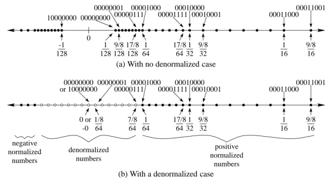
The first special case is for dealing with very small values. Let’s go back to the 8-bit representation we’ve been studying. If we plot the small numbers that can be represented exactly on the number line, we get the distribution illustrated in Figure 3.2(a). The smallest representable positive number is

(bit pattern 00000000), and the largest representable negative number is

(bit pattern 10000000). These are small numbers, but when we look at Figure 3.2(a), we see an anomaly: There is a relatively large gap between them. And — notice — there is no exact representation of one of the most important numbers of all: zero!

To deal with this, the IEEE standard defines the denormalized numbers. The idea is to take the most closely clustered numbers illustrated in Figure 3.2(a) and spread them more evenly across 0. This will give us the diagram in Figure 3.2(b).

(32)

1 32 9/8 32 128 1 0001100000011001 1 16 9/8 16 64 1 17/8 64 128 9/8 0 17/8 128 00000000 00001111 10000000 128 -1 0000011100001000 0001000000010001 00000001

(a) With no denormalized case

1 32 9/8 32 64 1/8 positive normalized numbers 0001100000011001 64 7/8 1 16 9/8 16 negative normalized numbers denormalized numbers 64 1 17/8 64 0 or -0 00000001 00001000 00000111 000011110001000000010001 or 1000000000000000

(b) With a denormalized case

Figure 3.2: Distribution of small floating-point numbers with and without a denormalized case. Those closely-clustered numbers in Figure 3.2(a) are those whose exponent bits are all 0. We’ll change the meanings of these numbers as follows: When all exponent bits are 0, then the exponent is

, and the mantissa has an implied 0 before it. Consider the bit pattern : In a floating-point format

incorporating the denormalized case, this represents 0.010 . (Without the

denormalized case, this would represent 1.010

. The changes are in the bit before the mantissa’s

decimal point and in the exponent of .) Suppose we want to represent 0.005

in our 8-bit floating-point format with a denormalized case. We first convert our number into the form

. In this case, we would get 0.320 . Converting 0.320

to binary, we get approximately 0.0101001

. In the 8-bit format, however, we have only three mantissa bits, and so we would round this to 0.011

. Thus, we have 0.011

, and so our bit representation would be . This is just an approximation to the original number of 0.005

: It is about 0.00586

. Without the denormalized case, the best approximation would be much further off (0.00781

).

How would we represent 0? We go through the same process: Converting this into the form

, we get

. This translates into the bit representation .

Why

for the exponent? It would make more intuitive sense to use , since this is what the all-zeroes exponent is normally. We use

, however, because we want a smooth transition between the normalized values and the denormalized values. The least positive normalized value is

(bit pattern 0 0000 000). If we used for the denormalized exponent, then the largest denormalized value would be 0.111

,

which is roughly half of the smallest positive normalized value. By using the same exponent as for the smallest normalized case, the standard spreads the denormalized numbers evenly from the smallest positive normalized number to 0. Figure 3.2(b) diagrams this: The open circles, representing values handled by the denormalized case, are spread evenly between the solid circles, representing the numbers handled by the normalized case.

The word denormalized comes from the fact that the mantissa is not in its normal form, where a nonzero digit is to the left of the decimal point.

(33)

3.4 Representing multimedia 27

The denormalized case works the same for the IEEE standard floating-point formats, except that the exponent varies based on the format’s excess. In the 32-bit standard, for example, the denormalized case is still the case when all exponent bits are zero, but the exponent it represents is

(since the normalized case involves an excess-127 exponent, and so the lowest exponent for normalized numbers is

).

Nonnumeric values (optional)

The IEEE standard’s designers were concerned with some special cases — particularly, computations where the answer doesn’t fit into the range of defined numbers. To address such possibilities, they reserved the all-ones exponent for the nonnumeric values. They designed two types of nonnumeric values into the IEEE standard.

If the exponent is all ones and the mantissa is all zeroes, then the number represents infinity or negative infinity, depending on the sign bit. Essentially, these two values are to represent numbers that have gone out of bounds. This value results from an overflow; for example, if you doubled the largest positive value, you would get infinity. Or if you divide 1 by a tiny number, you would get either infinity or negative infinity.

If the exponent is all ones, and the mantissa has some non-zero bits, then the number represents “not a number,” written as NaN. This represents an error condition; some situations where this occurs include finding the square root of , computing the tangent of , and dividing 0 by 0.

3.4 Representing multimedia

Programs often deal with much more complex data than characters, integers, and real numbers. In this section, we’ll look at the representation of images, video, and sound.

3.4.1 Images: The PNM format

Most techniques for representing images work by first breaking the image into a grid of pixels; each pixel is a small atom of color in the overall image. The word pixel comes from picture element. (This isn’t the only way to represent an image: An important alternative is to represent the image by component shapes. This works well for computer-generated drawings, but it works poorly for photographs.)

There are many different formats for representing images. We’ll look at one of the simplest: the PNM format. (PNM stands for Portable aNyMap.) In this format, we represent a picture as a sequence of ASCII characters. P1 7 7 0 0 0 0 0 0 0 0 1 1 1 1 0 0 0 1 0 0 0 0 0 0 1 1 1 0 0 0 0 1 0 0 0 0 0 0 1 0 0 0 0 0 0 0 0 0 0 0 0

The file begins with the format type — in this case, it is “P1” to indicate a black-and-white image. The next line provides the width and height of the image in pixels. The rest of the file contains a sequence of ASCII 0’s and 1’s, representing each pixel starting in the upper left corner of the image and going in left-to-right, top-down order. A 1 represents a black pixel, while a 0 represents a white pixel. In this example, the image is a image that looks like the following.