Asymptotic Behavior of Near Critical Branching
Processes and Modeling of Cell Growth Data
Dominik Reinhold
A dissertation submitted to the faculty of the University of North Carolina at Chapel Hill in partial fulfillment of the requirements for the degree of Doctor of Philosophy in the Department of Statistics and Operations Research (Statistics).
Chapel Hill 2011
Approved by:
Advisor: Amarjit Budhiraja
Advisor: M. Ross Leadbetter
Reader: Shankar Bhamidi
c
2011
Abstract
DOMINIK REINHOLD: Asymptotic Behavior of Near Critical Branching Processes and Modeling of Cell Growth Data.
(Under the direction of Amarjit Budhiraja and M. Ross Leadbetter.)
This dissertation is composed of two parts, a theoretical part, in which certain asymp-totic properties of near critical branching processes are studied, and an applied part, consisting of statistical analysis of cell growth data.
First, near critical single type Bienaym´e-Galton-Watson (BGW) processes are con-sidered. It is shown that, under appropriate conditions, Yaglom distributions of suitably scaled BGW processes converge to that of the corresponding diffusion approximation. Convergences of stationary distributions for Q-processes and models with immigration to the corresponding distributions of the associated diffusion approximations are estab-lished as well. Moreover, convergence of Yaglom distributions of suitably scaled multitype subcritical BGW processes to that of the associated diffusion model is established.
Next, near critical catalyst-reactant branching processes with controlled immigration are considered. The catalyst population evolves according to a classical continuous time branching process, while the reactant population evolves according to a branching process whose branching rate is proportional to the total mass of the catalyst. Immigration takes place exactly when the catalyst population falls below a certain threshold, in which case the population is instantaneously replenished to the threshold. A diffusion limit theorem for the scaled processes is established, in which the catalyst limit is a reflected diffusion and the reactant limit is a diffusion with coefficients depending on the reactant.
diffusions, but where the evolution of the catalyst is accelerated by a factor of n, we es-tablish a scaling limit theorem, in which the reactant process is asymptotically described through a one dimensional SDE with coefficients depending on the invariant distribution of the catalyst reflected diffusion. Convergence of the stationary distribution of the scaled catalyst branching process (with immigration) to that of the limit reflected diffusion is established as well.
Acknowledgments
I am very grateful to my advisor Professor Amarjit Budhiraja for all his encourage-ment and patience throughout my studies. His enthusiasm for research and encourage-mentoring helped making my stay in Chapel Hill an enormously rewarding and enjoyable experience. He was always available for short and long conversations, which were of great importance for my understanding and finishing of this dissertation.
I am thankful to my advisors Professors M. Ross Leadbetter and Budhiraja for giving me the opportunity to participate in the projectEmerging Frontiers in 3-D Breast Cancer Tissue Test Systems, part of which is discussed in this dissertation. Their experience and
advice was of great importance.
Next, I would like to thank the other members of my committee, Professors Shankar Bhamidi, Jan Hannig, and Chuanshu Ji, for their valuable comments on this dissertation. Special thanks go to Professor Bhamidi for all his suggestions and conversations with me. Faculty, staff, and my fellow students played an important role in making my stay in Chapel Hill a great experience, and I am very thankful to them.
Contents
Abstract . . . iii
List of Tables . . . viii
List of Figures . . . ix
1 Introduction . . . 1
1.1 Notation . . . 7
2 Asymptotic Behavior of Near Critical Branching Processes . . . 10
2.1 Introduction and Main Results . . . 10
2.2 Proofs: Single Type Case. . . 22
2.3 Proofs: Multitype Case. . . 32
3 Catalyst-Reactant Branching Processes . . . 39
3.1 Introduction and Main Results . . . 39
3.2 Proof of Proposition 3.1.1 . . . 44
3.3 Proof of Theorem 3.1.2 . . . 45
4 Stochastic Averaging Under Fast Catalyst Dynamics . . . 61
4.1 Fast Catalyst Diffusion . . . 63
4.2 Convergence of Invariant Distributions . . . 63
4.4 Proof of Theorem 4.1.1 . . . 65
4.5 Proof of Theorem 4.2.1 . . . 71
5 Modeling Cancer Cell Behavior as a Function of Substrate Stiffness 85 5.1 Introduction . . . 85
5.2 Metabolic Activity and Viability . . . 88
5.2.1 Preparation and Measurements . . . 88
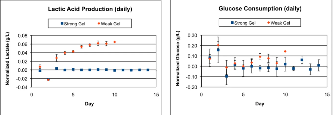
5.2.2 Lactic Acid Production and Glucose Consumption . . . 89
5.2.3 Alamar Blue Assay . . . 90
5.2.4 Live/Dead Cell Viability Assay . . . 91
5.3 Morphology Imaging . . . 91
5.3.1 Statistical Modeling . . . 93
5.4 Discussion . . . 100
6 Appendix . . . 103
List of Tables
5.1 Estimates of the coefficients of the model forCOT . . . 96
5.2 Estimates of the coefficients of the model for ln(N) . . . 96
5.3 Estimates of the coefficients of the model for ln(AC) . . . 98
List of Figures
5.1 Normalized lactic acid production and glucose consumption . . . 90
5.2 Alamar Blue assay results . . . 91
5.3 Live/Dead assay results . . . 92
5.4 Example of errors introduced by the image processing protocol . . . 93
5.5 Increase inCOT as a function of agarose content from day 6 - 8 . . . 95
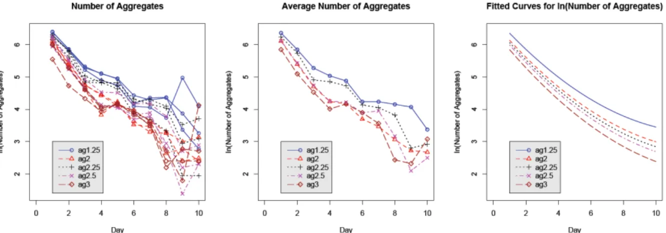
5.6 Natural logarithm of number of aggregates over days 1 - 10 . . . 97
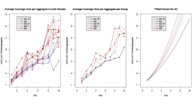
5.7 Average coverage area of aggregates over days 1 - 8 . . . 98
5.8 Increase in ln(AC) as a function of agarose content from day 6 - 8 . . . 99
Chapter 1
Introduction
This dissertation is composed of two parts, a theoretical part, in which we study certain asymptotic properties of near critical branching processes, and an applied part, consisting of statistical analysis of cell growth data as part of the EFRI-CBE1 project
Emerging Frontiers in 3-D Breast Cancer Tissue Test Systems.
Branching processes have been studied extensively (see [1]) and have proved to be useful for modeling population dynamics in a variety of fields (see [15]). We study here the so-called Bienaym´e-Galton-Watson (BGW) processes, their multidimensional analogues, and continuous time catalyst-reactant branching processes. Roughly speaking, a BGW process is a Markov chain {Zn}n∈N0 with state space N0 with the following behavior.
The process starts with Z0 particles; each of the Zn particles alive at time n lives for
one unit of time and then dies, giving rise to l offspring particles with probability pl,
l ∈ N0, where {pl}l∈N0 is a probability distribution, the so-called offspring distribution.
In the multitype setting of k-BGW processes (k ∈ N), Zn is a k-dimensional vector
model populations with a certain kind of interaction (see [14] and references therein). More precisely, they describe dynamics where the catalyst population directly affects the activity level of an associated reactant population. In our model, roughly speaking, we consider a population of catalyst particles, which evolves according to a classical continuous time branching process with constant branching rate (the life time of each particle is exponentially distributed, instead of being constant as in the setting of BGW processes) with a specific form of immigration, and a reactant population whose branching rate is proportional to the total mass of the catalyst population.
We first describe our main results for BGW processes in the single and multitype setting. This work has appeared as “Some asymptotic results for near critical branching processes” in Communications on Stochastic Analysis in 2010 ([5]). Next, we describe our results for catalyst-reactant branching processes, and finally give a description of a proof-of-principle study from the EFRI-CBE project ([2]). This project involves re-searchers from multiple departments and universities, and the work presented here has been conducted jointly with multiple collaborators.
Consider first the single type setting (i.e. k = 1) of BGW processes. Depending on the mean m of the offspring distribution, the BGW process is referred to as subcritical, critical, or supercritical, according to whether m <1,m= 1, or m >1, respectively.
We are concerned with the scaled processes ˆZt(n) = n1Zb(n)ntc, where {Z(n)}
n∈N is a sequence of BGW processes, with offspring means mn tending to 1, as n → ∞. Our
primary interest is in the steady state behavior of ˆZt(n) as t → ∞. However, in order to obtain a meaningful asymptotic limit (ast → ∞), one needs to suitably reformulate this question since, as is well known, for mn > 1, ˆZt(n) tends to infinity on the set of
non-extinction ast→ ∞, and formn ≤1, ˆZ (n)
t eventually becomes extinct (see [1]). There are
two common approaches to address the problem of certain extinction of ˆZ(n) in the (sub-)
speaking, the conditioning can either be on non-extinction at the present time or in the distant future. The state process ˆZ(n) under these two conditionings leads to different limiting distributions as t → ∞. The first is the so-called quasi-stationary distribution of ˆZ(n), while the second is the stationary distribution of the Q-process associated with
ˆ
Z(n) (see Section I.14 of [1]).
The second approach to deal with eventual extinction (in the (sub-) critical setting) is to introduce an immigration component, namely, in each generation a (random) number of particles that are indistinguishable from the original set of particles is added to the population. The immigration component in particular ensures that the resulting scaled state process ˆZ(n) has a non-degenerate stationary probability distribution.
In the supercritical case, in order to obtain a nontrivial limiting behavior, one typically conditions on the intersection of the event of non-extinction at the present time and the event of eventual extinction. It turns out that a supercritical BGW process with this conditioning has the same distribution as a certain subcritical process. This observation enables us to transfer the results for subcritical processes to supercritical processes.
It is well known (see [10], [20]) that, under suitable conditions, ˆZ(n) converges weakly to a diffusionξ. Such a result implies convergence of finite time statistics of ˆZ(n)to those
of ξ, but does not provide any information on the relationship between the time asymp-totic behaviors of ˆZ(n) and ξ. The main goal of this work is to make such relationships
mathematically precise. In particular, we show that the time asymptotic distribution of ˆ
Zt(n) under suitable conditioning converges to that ofξt under a similar conditioning, as
In addition to the results in the single type setting, we have results in a multitype setting as well. Here, the mean offspring matrixM plays an analogous role to the mean m in the single type case. The (i, j)th component of M is the expected number of type
j offspring from a single particle of type i in one generation. The Perron-Frobenius theorem shows that, under suitable conditions, there exists an eigenvalue ρ ∈R+ of M,
such that the absolute value of any other eigenvalue is strictly smaller than ρ. Similar to the single type case, the process is referred to as subcritical, critical, or supercritical, according to whether ρ < 1, ρ = 1, or ρ > 1, respectively. We establish a convergence result for quasi-stationary distributions analogous to that in the single type setting.
We next study catalyst-reactant branching processes. As in the BGW setting, we consider sequences of catalyst and reactant processes, which are denoted by {X(n)}
n∈N and {Y(n)}
n∈N, respectively. Both X(n) and Y(n) are subcritical, with offspring means tending to 1, as n → ∞, and both processes start with n particles. In typical settings (see e.g. [14]), the catalyst evolution is modeled through a classical continuous time branching process, and consequently population dynamics are described until the time the catalyst becomes extinct. In contrast, our work considers a setting where the catalyst population is maintained above a positive threshold through a specific form of controlled immigration. More precisely, when the catalyst population X(n) drops below n, it is
instantaneously restored to level n.
arise from predator-prey models in ecology, where one may be concerned with the restora-tion of popularestora-tions that are close to extincrestora-tion by reintroducing species when they fall below a certain threshold. In our work, the motivation for the study of such controlled immigration models comes from problems in chemical kinetics where one wants to keep the level of a catalyst above a certain threshold in order to maintain a desirable level of reaction activity.
We will establish a diffusion limit theorem for the scaled processes ( ˆXt(n),Yˆt(n)) := (1nXnt(n),n1Ynt(n)). The limit process (X, Y) will be such that X is a reflected diffusion with reflection at 1, and Y is a diffusion with coefficients depending on X. The driving Brownian motions in the two diffusions will be independent.
The catalyst and reactant populations considered in the results described above evolve on a comparable time scale in the sense that the branching rates of both X(n) and Y(n)
program, which is to establish the convergence of the stationary distribution of the scaled catalyst process ˆX(n) to that of the limit reflecting diffusion X.
The enormous potential of a 3D test system is in the ability to construct cells in a biomaterial substrate in a spatially meaningful manner that allows cellular behavior that is more indicative of behavior in native tissue than a 2D system, thus allowing rapid discoveries of therapies and preventatives for an array of diseases. This proof-of-principle work demonstrates the possibility of using image processing and statistical modeling to describe pseudo-3D cancer systems in a non-destructive and spatio-temporal manner.
The chapters are organized as follows. At the end of this section we list notation that will be used throughout the dissertation.
In Chapter 2 we study asymptotic behavior of single and multitype BGW processes. Chapter 3 is concerned with the weak convergence of suitably scaled catalyst-reactant branching processes to (reflected) diffusions.
In Chapter 4 we establish an averaging principle under fast catalyst dynamics and also study convergence of invariant distributions of the catalyst processes.
In Chapter 5, we summarize results from a proof-of-principle study from the EFRI-CBE project.
Chapter 6 is an appendix in which we provide proofs of some auxiliary lemmas that are used in preceding chapters.
1.1
Notation
N:={1,2, . . .}
N0 :={0,1,2, . . .}
Nk:={i≡(i1, . . . , ik)0|iα ∈N,1≤α≤k}
Nk0 :={i≡(i1, . . . , ik)0|iα ∈N0,1≤α≤k}
Rk+:={i≡(i1, . . . , ik)0|iα ∈[0,∞),1≤α≤k}
R≥1 := [1,∞)
Z:={. . . ,−2,−1,0,1,2, . . .}
0:= (0,0, . . . ,0)0
1:= (1,1, . . . ,1)0
δij :=
1 if i=j 0 otherwise
1A(x) :=
1 if x∈A 0 otherwise
eα := (δ1α, . . . , δkα)0
si :=Qk
α=1s iα
α, for i= (i1, . . . , ik)0 ∈Nk0 and s= (s1, . . . , sk)0 ∈Rk+.
Cl(
S): The set of l-times continuously differentiable, real-valued functions onS.
Cl
c(S): The set of l-times continuously differentiable, real-valued functions on S that
have compact support.
C(R+ :S): the space of continuous functions from R+ toS.
D(R+: S): the space of c`adl`ag (or RCLL – right continuous with left limits) functions
fromR+ toS.
P(Ω): The set of probability measures on a fixed measurable space (Ω,F).
Sn:={nl|l ∈N0}
S(n)X :={ l
S(n)Y :={ l
n|l∈N0}
S(n)Z :={ l
n|l∈Z}
W(n) :=S(n)X ×S (n)
Y ×S
(n) Z
W:=R≥1×R+×R
|| · ||: the Euclidean norm onRk.
|X|∗,t := sup 0≤s≤t
Chapter 2
Asymptotic Behavior of Near Critical Branching
Processes
The following results appeared as “Some asymptotic results for near critical branching processes” in Communications on Stochastic analysis in 2010 ([5]).
2.1
Introduction and Main Results
Consider a population consisting ofk types of particles whose evolution is described in terms of a discrete time multitype (k-type) Bienaym´e-Galton-Watson (k-BGW) process – such a process is a Markov chain {Zp}p∈N0 on N
k
0, with the vector Zp representing
the number of particles of each type in generation p. We are interested in the long time behavior of the scaled process 1pZbptc, t ≥ 0, when the k-BGW process is close to
criticality. More precisely, we consider a sequence of BGW processes {Zp(n), p ∈N0}n∈N such that, as n becomes large, the processes approach criticality. It is well known (see [10], [20]) that, under suitable conditions, the process Xt(n) = 1
nZ (n)
bntc, t ≥ 0, converges weakly to a diffusion ξ. (We note here that in Chapter 1 the scaled process n1Zb(n)ntc was denoted by ˆZt(n). However, throughout this chapter we will useXt(n) to denote this scaled process.) Such a result implies convergence of finite time statistics of X(n) to those of
time asymptotic distribution of Xt(n) with suitable conditioning converges to that of ξt
with a similar conditioning, as n → ∞ (see Theorems 2.1.4 and 2.1.7). An analogous result for models with immigration (where no conditioning is required) is also established (Theorem 2.1.10). The results say that the long time behavior of a BGW process is well approximated by that of the corresponding diffusion limit ξ. Most of the results in this work are for single type BGW processes, namely for the case k = 1. Similar results can be obtained in multitype settings and we consider one such result in Theorem 2.1.18.
When k= 1, the transition probabilities of a BGW process {Zp} can be written as
p(i, j) =P(Zp+1 =j|Zp =i) =
p∗i
j if i≥1, j ≥0,
δ0j if i= 0, j ≥0,
(2.1.1)
where{pl}l∈N0 is a given probability function – the offspring distribution of each particle
– and {p∗i
l }l∈N0 is thei-fold convolution of{pl}l∈N0. The process starts withZ0 particles;
each of theZnparticles alive at timenlives for one unit of time and then dies, giving rise
to l offspring particles with probability pl, l ∈ N0. The particles behave independently
of each other and of the past.
Depending on the meanmof the offspring distribution, BGW processes can be divided into three cases: subcritical, critical, and supercritical, according to whether m < 1, m= 1, or m >1, respectively.
Consider a sequence of processes Z(n) described as follows. IfZ(n)
0 = 1, thenZ (n)
1 has
the probability generating function (pgf)
F(n)(s) = ∞
X
l=0
p(n)l sl, s ∈[0,1], (2.1.2)
with mean mn and varianceσ2n, where {p (n)
l }l∈N0 is the offspring distribution ofZ
denote the pth iterate of F(n) byF(n)
p , i.e. for s∈[0,1] andp≥0
F0(n)(s) =s, Fp+1(n)(s) =F(n)(Fp(n)(s)).
Let qn be the extinction probability of Z(n) starting from a single particle, i.e. qn =
P(Zp(n)= 0 for some p∈N|Z0(n) = 1). Let
Xt(n) := 1 nZ
(n)
bntc, t ∈R+; (2.1.3)
then {Xt(n)}t∈R+ is an Sn := {
l
n|l ∈ N0} valued (time inhomogeneous) Markov process
with sample paths in D(R+ : Sn), the space of c`adl`ag functions from R+ := [0,∞) to
Sn. Throughout, Sn is endowed with the discrete topology and, given a metric space S,
D(R+ :S) is endowed with the usual Skorohod topology. Space of probability measures
on a metric space S will be denoted by P(S).
Condition 2.1.1. (i) For eachn, p(n)0 >0, p(n)0 +p(n)1 < qn, mn= 1 +cnn, cn∈(−n,∞)\
{0}, and σ2n < ∞. (ii) As n → ∞, cn → c ∈ R\ {0} and σ2n → σ2 ∈ (0,∞). (iii)
The family of functions {F(n)00}
n∈N is equicontinuous at 1. (iv) Asn → ∞,
P
l:l>√n(l−
mn)2p (n)
l →0, and X (n)
0 converges in distribution to some µ∈ P(R+).
Condition 2.1.1 (i) ensures that, as n → ∞, mn → 1, and thus the processes
ap-proach criticality without being critical. The case where c <0 will be referred to as the subcritical case while c > 0 corresponds to the supercritical case. Condition 2.1.1 (iii) will be used in the study of the supercritical case in Theorem 2.1.4. Condition 2.1.1 (iv) is needed for the diffusion approximation result in Theorem 2.1.2.
We now recall a well known weak convergence result for X(n) (see [12], [20, Theorem
4.2.2]), which describes the asymptotic behavior of X(n), as n → ∞, over any fixed
Theorem 2.1.2. [12, 20] Assume Condition 2.1.1. Then X(n) converges weakly in D(R+:R+) to the unique (in law) diffusion process ξ with generator
(Lf)(x) =xcf0(x) + 1 2xσ
2f00
(x), f ∈C2(R+), x∈R+, (2.1.4)
and initial distribution (i.e. probability law of ξ0) equal to µ.
We are concerned with the study of relationships between the steady state behavior of X(n) and that of ξ. However, one needs to suitably interpret the term “steady state”
since, as is well known, as t → ∞, for mn >1, X (n)
t tends to infinity on the set of
non-extinction, and formn ≤1,X (n)
t eventually becomes extinct (see [1]). There are two well
studied approaches for formulating time asymptotic questions in the subcritical case. The first is to condition the processes X(n) on non-extinction, where, loosely speaking, the conditioning can either be on non-extinction at the present time or in the distant future. The state processX(n) under these two conditionings has different limiting distributions
as t → ∞. The first is called the Yaglom distribution of X(n), while the second is
the stationary distribution of the Q-process associated with X(n) (see Section I.14 of
[1]). The second approach for obtaining a nontrivial time asymptotic behavior is to introduce an immigration component. Namely, in each generation a (random) number of particles that are indistinguishable from the original set of particles is added to the population. The immigration component in particular ensures that the resulting scaled state process, denoted by V(n), has a non-degenerate stationary distribution. For the
supercritical case, a common approach is to reduce the problem to that of a subcritical setting by conditioning on the event of eventual extinction. The so conditioned state process X(n) has the same law as the state process corresponding to a certain subcritical
prove convergence of stationary distributions.
We begin by describing results for models without immigration. For a Markov process
{Yt}t∈R+ with initial value Y0 = y, we write P(Yt ∈ ·) as Py(Yt ∈ ·). Similarly, when
the distribution of Y0 is µ, we write P(Yt ∈ ·) as Pµ(Yt ∈ ·). Similar notations will be
used for conditional expectations. Let S be a subset of Rk
+, for some k ∈ N. When S is
endowed with a topology, we will denote by B(S) the σ-field generated by the open sets of S. Let Y ≡ {Yt}t∈R+ be an S-valued Markov process such that 0 ∈S is an absorbing
state.
Definition 2.1.1. (i) A quasi-stationary distribution (qsd) for Y is a probability distri-bution µ on (S,B(S)) such that Pµ(Yt ∈ B|t < TY < ∞) = µ(B) for all B ∈ B(S) and
t≥0, where TY := inf{t|Yt=0}.
(ii) If for all y ∈ S\ {0}, as t → ∞, Py(Yt ∈ ·|t < TY < ∞) converges weakly to some
probability measure µ on (S,B(S)), thenµ is called the Yaglom distribution ofY.
The following result follows from [23] and Proposition 2.3.2.1 of [24].
Theorem 2.1.3. [23, 24] The Yaglom distribution of ξ exists and is Exponential with density
f(x) = 2|c| σ2 exp
−2|c|
σ2 x
, x≥0. (2.1.5)
Our first result, Theorem 2.1.4 below, says that the Yaglom distribution of X(n)
approaches that of ξ, as n → ∞. Note that the existence of the Yaglom distribution of X(n) in the subcritical case is a direct consequence of Theorem V.4.2 of [1].
Theorem 2.1.4. Assume Condition 2.1.1. For each n, X(n) has a Yaglom distribution ν(n). This distribution is also a qsd, and it converges weakly to the Yaglom distribution ν of ξ.
not being extinct in the “distant future”. We will see that in this case a somewhat differ-ent asymptotic behavior emerges. For this result we restrict ourselves to the subcritical case (i.e. cn<0). We begin with the definition of a Q-process (see [1], [23]).
Let ˆΩ = D(R+ : R+) and ˆF be the corresponding Borel σ-field (with the usual
Skorohod topology). Denote by {Ft}t∈R+ the canonical filtration on ( ˆΩ,Fˆ), i.e. Ft =
σ(πs : s ≤ t), where πs(x) =xs for x ∈ Ω. We denote by ˆˆ P (n)
µ the measure induced by
X(n) on ( ˆΩ,Fˆ) whenZ0(n) has distribution µ(supported on N). Let T := inf{t|πt = 0}.
By Lemma 6.0.3 in the appendix, there is a probability measure Pµ(n)↑ on ( ˆΩ,Fˆ) such
that, as s → ∞, ˆPµ(n)(Θ|T > s) → P(n)
↑
µ (Θ), for all Θ ∈ Ft, t ∈ R+. Furthermore if
{Zk(n)↑}k∈N0 is a Markov chain with state spaceN, l-step transition function
p(n)l ↑(i, j) = P(Zl(n) =j|Z0(n) =i)j im
−l
n , i, j ∈N,
and initial distribution µ, then Pµ(n)↑ is the law of {X (n)↑
t }t∈R+, where X
(n)↑
t := 1nZ
(n)↑ bntc, t∈R+. The processZ(n)↑ [respectivelyX(n)↑] is called the Q-process associated withZ(n)
[respectively X(n)]. Q-processes associated with branching processes can be interpreted
as branching processes conditioned on being never extinct.
Next, we introduce the Q-process associated with the diffusionξ from Theorem 2.1.2. Denote by Pξ,x the measure induced by ξ on ( ˆΩ,Fˆ), where ξ(0) = x >0. The following
theorem is contained in [23].
Theorem 2.1.5. [23] There is a probability measure Pξ,x↑ on ( ˆΩ,Fˆ), such that for all t∈R+ andΘ∈ Ft, Pξ,x(Θ|T > s) converges to P
↑
ξ,x(Θ), as s→ ∞. Let ξ
↑ be the unique weak solution of the SDE
dξt↑ =cξt↑dt+
q
σ2ξ↑
tdBt+σ2dt, ξ
↑
0 =x,
( ˆΩ,Fˆ).
The process ξ↑ is referred to as the Q-process associated withξ. The following result (see [23], Section 5.2) says that the process ξ↑ has a unique stationary distribution, ν↑, which is given as the convolution of two copies of the exponential distribution ν with density as in (2.1.5).
Theorem 2.1.6. [23] Assume c < 0. As t → ∞, for every initial condition x, ξt↑ converges in distribution to a random variable ξ∞↑ , whose distribution, denoted by ν↑, is the convolution of two copies of the Yaglom distribution ν. In particular, ν↑ has density
f(x) =
2c σ2
2
xexp
2c σ2x
, x≥0. (2.1.6)
Our next result shows that the time asymptotic behavior of the Q-process associated withX(n)can be well approximated by that of the Q-process associated with the diffusion approximation of X(n). Note that the existence of the stationary distribution of the
Q-process X(n)↑ is immediate from Theorem I.14.2 in [1].
Theorem 2.1.7. Assume Condition 2.1.1 and that cn < 0 for all n ∈ N. For each n,
Xt(n)↑ converges in distribution, as t→ ∞, to a random variable X∞(n)↑. The distribution ν(n)↑ of X∞(n)↑ is the unique stationary distribution of theSn valued Markov process X(n)↑.
As n → ∞, ν(n)↑ converges weakly to ν↑.
We now describe the results for BGW processes with immigration. Let F and G be pgf’s ofN0 valued random variables. A Bienaym´e-Galton-Watson branching process with
immigration corresponding to (F,G) (referred to as a DBI(F, G) process), is a Markov chain {Yn}with state-space N0 and transition probability function described in terms of
the corresponding pgf: Given Y0 =i∈N, the pgf H(i,·) of Y1 isH(i, s) =
P∞
j=0P(Y1 =
Let G(n) be a sequence of pgf’s, and consider a sequence of DBI(F(n), G(n)) processes Y(n).
Condition 2.1.8. (i) There are ι0, κ0 ∈(0,∞) such that, for all n ∈N, G(n)
0
(1) =ιn≥
ι0 and G(n)
00
(1) = κn ≤ κ0. (ii) As n → ∞, ιn → ι. (iii) There is a τ0 ∈ [0,∞) such
that, for all n ∈N, F(n)000(1) =τ
n< τ0.
Let Vt(n) := n1Yb(n)ntc, t ∈ R+. The proof of the following theorem is easy to establish
using [23] and [25, Theorem 2.1].
Theorem 2.1.9. Assume Conditions 2.1.1 and 2.1.8 and that c < 0. Suppose that V0(n) converges in distribution to someµ∈ P(R+). ThenV(n) converges weakly inD(R+ :R+)
to the process ζ which is the unique weak solution of
dζt=cζtdt+
p
σ2ζ
tdBt+ιdt, t≥0,
where ζ0 has distribution µ. The Markov process ζ has a unique stationary distribution
η, which is a gamma distribution with parameters 2ι/σ2 and σ2/(2|c|), i.e., ηhas density
g given as
g(x) = xσ2ι2−1
exp−x2σ|c2|
σ2
2|c|
2ι
σ2
Γ σ2ι2
, x >0.
We are interested in the long time behavior of the scaled processes V(n) as they
approach criticality. Our main result is the following. Note that the existence of the stationary distribution of V(n) is immediate from [34], p. 414.
Theorem 2.1.10. Assume Conditions 2.1.1 and 2.1.8 and that cn < 0 for all n ∈ N.
For each n ∈ N, V(n) has a unique stationary distribution η(n), and as n → ∞, η(n)
As noted earlier in the introduction, results similar to Theorems 2.1.4, 2.1.6, and 2.1.10 can be established for multitype settings as well. To illustrate the key ideas involved, we only discuss one case in detail, namely the convergence of the Yaglom distribution in the setting of a subcritical multitype process. We begin with some notation and definitions. Let{Zj(n), j ∈N0}n∈N be a sequence ofk-BGW processes with transition mechanism described below. Let C := [0,1]k, e
α := (δ1α, . . . , δkα)0 be the αth canonical
basis vector, and si := Qk
α=1s iα
α, for i = (i1, . . . , ik)0 ∈ Nk0 and s = (s1, . . . , sk)0 ∈ Rk+.
Similar to the single type case, the evolution of Zj(n) = (Zj,1(n),· · ·Zj,k(n))0 is described as follows. For any α = 1, . . . , k, each of the Zj,α(n) type α particles alive at time j (if any) lives for one unit of time and then dies, giving rise to a number of offspring particles, represented by l= (l1, . . . , lk),lβ being the number of type β offspring, with probability
p(n)(e
α,l). The particles behave independently of each other and of the past. The
probability law of Z(n) is given in terms of the pgf F(n)(s) := (F(n)
(1)(s), . . . , F (n) (k)(s)),
s ∈ C, where F(α)(n)(s) := P j∈Nk0p
(n)(e
α,j)sj, 1 ≤ α ≤ k, s ∈ C. Let m (n)
αβ = EeαZ
(n) 1,β be
the expected number of typeβoffspring from a single particle of typeαin one generation. Then thek×kmatrixM(n) = (mαβ(n))α,β=1,...,k is called themean matrix ofZ(n). Note that
m(n)αβ = ∂F
(n) (α)
∂sβ (1),where the partial derivative is understood to be the left hand derivative.
The processes Z(n) will be assumed to have a uniformly strictly positive mean matrix
M(n), by which we mean that there exist U ∈
N and a ∈ (0,∞) such that for every
n ≥ 1 ((M(n))U)
α,β ≥ a for all 1 ≤ α, β ≤ k. From the Perron-Frobenius Theorem it
then follows thatM(n)has a real, positive maximal eigenvalueρ
nwith associated positive
left and right eigenvectors v(n) and u(n), respectively, which, without loss of generality, are normalized so that u(n)0v(n) = 1 and u(n)01 = 1 (see [1]). The maximal eigenvalue ρn plays a similar role in the classification of the k-BGW process as the mean played
will consider the subcritical case, namely for alln ≥1ρn ∈(0,1), and study the behavior
of quasi-stationary and Yaglom distributions of the scaled processX(n)(t) = Z
(n) bntc
n ,t≥0,
as ρn→1.
Condition 2.1.11. For each n≥1, E1(||Z (n)
1 ||log||Z (n)
1 ||)<∞.
The existence of the Yaglom distribution of X(n) is assured by the following result,
which is a consequence of Theorem V.4.1 of [1] (see also Theorem V.4.2 therein). We give a proof in Section 2.3.
Theorem 2.1.12. Assume Condition 2.1.11. For each n ∈ N, X(n) has a Yaglom distribution ν(n). This distribution is also a qsd.
Condition 2.1.13. There exist b, d ∈ (0,∞) such that for all n ∈ N (i)
P
αβγ∂ 2F(n)
(α)(1)/∂sβ∂sγ ≥b, and (ii)
P
α,β,γ,δ∂ 3F(n)
(α)(1)/∂sβ∂sγ∂sδ ≤ d, where α, β, γ, δ
in the above sums vary over {1, . . . , k}.
Part (i) of the assumption can be interpreted as a non-degeneracy condition, and part (ii) says that the third moments of the offspring distributions are uniformly bounded in n.
The assumption on convergence of means translates into the following requirement in the multitype setting.
Condition 2.1.14. For some strictly positive matrix M and each n ∈ N, M(n) =M+
C(n)
n , and limn→∞C
(n) =C. The maximal eigenvalues ρ
n of M(n) are of the form ρn =
1 + cn
n, with cn ∈ (−n,0) and limn→∞cn = c ∈ (−∞,0). Moreover, M has maximal
eigenvalue 1 with corresponding eigenvectors v = limv(n) and u = limu(n). Finally,
v0Cu=c.
Example 2.1.1. Let C(n) = c
nI, where I is the identity matrix and cn ∈ (−n,0) such
that cn →c∈(0,∞). Let M be a strictly positive matrix with maximal eigenvalue equal
Let
σi,j(n)(l) = X
r∈Nk0
(ri−m (n)
li )(rj −m (n) lj )p
(n)(e l,r).
The following condition is analogous to the assumption on convergence of variances in the single type case.
Condition 2.1.15. As n → ∞, σi,j(n)(l) → σi,j(l) for all 1 ≤ i, j, l ≤ k and Q := 1
2
Pk l=1vlu
0σ(l)u>0, where σ(l) is the matrix with (i, j)th entry σ i,j(l).
The following diffusion approximation result can be established along the lines of Theorem 4.3.1 of [20] and Theorem 9.2.1 of [10]. We provide a sketch in Section 2.3.
Theorem 2.1.16. Assume Conditions 2.1.13, 2.1.14, and 2.1.15. Suppose that the
dis-tribution of X(n)(0) converges to some µ∈ P(R+k). Let µ1 ∈ P(R+) be given as
µ1(A) = µ{x∈Rk+|x
0
u∈A}, A∈ B(R+). (2.1.7)
Let ζ(n) = X(n)0u(n). Then ζ(n) converges weakly in D(R+ : R+) to the unique (in law)
diffusion ζ with initial distribution µ1 and generator L˜ given as
( ˜Lf)(x) =cxf0(x) +Qxf00(x), f ∈Cc∞(R+), x∈R+. (2.1.8)
Furthermore, for any t0 ∈ (0,∞), the process X(n,0), defined by X(n,0)(t) =X(n)(t0+t),
t≥0, converges weakly to X(0) =vζ(0), where ζ(0)(t) =ζ(t
0+t), t ≥0.
The process X(0) is a Markov process with state space S
v = {θv|θ ≥ 0} and can
be formally regarded as the limit of X(n). Indeed, if the support of µ is contained in
Sv, then, noting that u0v = 1, we see that the law of vζ(0) equals µ, and that in fact
with the Yaglom distribution of the Sv valued Markov process X(0) and its relation to
the Yaglom distribution of X(n). For that it will be convenient to regard a probability measure on Sv as one on Rk+. Denote by ˜ν the Exponential distribution with density
f(x) = |c|Q−1exp(−|c|Q−1x),x≥0. Theorem 2.1.3 says that the Yaglom distribution of
ζ(0) is given by ˜ν. SinceX(0) =vζ(0), the Yaglom distribution of X(0) exists as well and
equals the distribution of vY, where Y has distribution ˜ν. Thus, we have the following:
Theorem 2.1.17. Assume Conditions 2.1.13, 2.1.14, and 2.1.15. The Yaglom
distribu-tion of ζ(0) exists and equals ν. Furthermore, the Yaglom distribution of˜ X(0), denoted by ν, exists and equals the distribution of¯ vY, where Y has distribution ν.˜
The following is our main result that relates the qsd’s and Yaglom distributions of X(n) to that of its “diffusion limit” X(0). Probability distributions similar to ¯ν have
previously been noted in the study of qsd’s of multitype BGW processes. In [1] (p. 191), a single critical BGW processZ (rather than a sequence of near critical BGW processes) is considered and it is shown that Zn/n conditioned on non-extinction converges to a
random variable that is concentrated on the ray{xvZ|x≥0}, wherevZ is the left
eigen-vector of the mean matrix of Z corresponding to the eigenvalue 1. In [35] (see Theorem 3 therein) the case whereZ is near critical and a somewhat differently (component wise) scaled process Z∗ is considered. The asymptotic behavior of Zn∗ conditioned on non-extinction, as n → ∞, and the offspring distribution approaches criticality, is related to the limiting distributions considered here. We remark that none of these results concern the setting of diffusion approximation, where time and space are scaled and one starts with a large number of particles.
Theorem 2.1.18. Assume Conditions 2.1.13, 2.1.14, and 2.1.15. The Yaglom
2.2
Proofs: Single Type Case.
In this section we give proofs of Theorems 2.1.4, 2.1.7, and 2.1.10. We begin with Theorem 2.1.4.
Proof of Theorem 2.1.4. In the subcritical case, it is immediate from Theorem V.4.2 of [1] thatX(n) has a Yaglom distributionν(n). A representation of the Laplace transform
of ν(n) in the subcritical or supercritical case is given in Lemma 2.2.1, below. Moreover, by Lemma 6.0.1 and (2.2.7), ν(n) is a qsd.
We now show that ν(n) converges weakly to ν. The first step is to establish the
representation for the Laplace transform of ν(n) given in Lemma 2.2.1 below. In the
subcritical case, define
Qk(n)(s) :=m−nk(Fk(n)(s)−1), s∈[0,1]. (2.2.1)
Then Q(n)k converges pointwise over [0,1], as k → ∞, to a continuous function Q(n) that
is positive on [0,1) (see [1], p. 40, Corollary I.11.1), i.e.
lim
k→∞Q
(n)
k (s) =: Q (n)
(s), s∈[0,1], (2.2.2)
whereQ(n)(s)>0 for s∈[0,1). The functionQ(n) will determine the Laplace transform
ofν(n) in the subcritical case. In the supercritical case, we proceed as follows. Note that,
sincep(n)0 >0, we have that qn >0. Also since mn >1, we haveqn ∈(0,1) and that qnis
the smallest root of F(n)(t) =t (see [1], Theorem I.5.1). Define ˜F(n)(s) :=qn−1F(n)(qns),
s ∈ [0,1]. Since F(n)(qn) = qn, each ˜F(n) is again a pgf and thus has a representation
˜
F(n)(s) = P∞
l=0p˜ (n)
l s
l, s ∈ [0,1], with P∞
l=0p˜ (n)
l = 1. In fact, ˜p (n)
l = p
(n)
l q
l−1
n , l ∈ N0.
The probability distribution {p˜(n)l } has mean ˜mn = qn−1F(n)
0
(qn)qn = F(n)
0
(qn) < 1 and
variance ˜σ2
n = ˜F(n)
00
(1)−m˜2
n+ ˜mn = qnF(n)
00
(qn)−m˜2n+ ˜mn. That F(n)
0
(qn) < 1 is a
consequence ofF(n)0(1)>1,F(n)(q
latter follows from the assumption thatp(n)0 +p(n)1 < qn. Let ˜Q (n)
k (s) := ˜m
−k n ( ˜F
(n)
k (s)−1),
s∈[0,1]. Then
lim
k→∞ ˜
Q(n)k (s) =: ˜Q(n)(s), s∈[0,1], (2.2.3)
and ˜Q(n) has the same properties as those of Q(n) in the subcritical case noted earlier.
Lemma 2.2.1. The Laplace transform ofν(n), R
[0,∞)e
−αxν(n)(dx), in the subcritical case,
is given as [Q(n)(0)−Q(n)(e−α/n)]/(Q(n)(0)) and, in the supercritical case as [ ˜Q(n)(0)−
˜
Q(n)(e−α/n)]/( ˜Q(n)(0)).
Proof. Consider first the subcritical case. Since TX(n) <∞ a.s., it suffices to show that,
for each α ≥0,
lim
t→∞E
i n
e−αXt(n)|X(n)
t >0
= Q
(n)(0)−Q(n)(e−α/n)
Q(n)(0) . (2.2.4)
Elementary calculations give
Ei n
e−αXt(n)|X(n)
t >0
= 1−An,t(e
−α/n)
An,t(0)
, (2.2.5)
where, forθ ∈[0,1],An,t(θ) = m
−bntc
n
1−hFb(n)ntc(θ)i
i
. Next,
lim
t→∞An,t(e
−α/n) = lim
t→∞m
−bntc
n 1−
i X k=0 i k
Fb(n)ntc(e−α/n)−1
k!
= −i lim
t→∞m
−bntc
n
Fb(n)ntc(e−α/n)−1=−iQ(n)(e−α/n),
(2.2.6)
where the second and third equalities follow from (2.2.2). In exactly the same way one sees that limt→∞An,t(0) =−iQ(n)(0).Combining the above observations we have (2.2.4),
Consider now the supercritical case. Similar to the subcritical case
Ei n(e
−αXt(n)|t < T
X(n) <∞) =
h
Fb(n)ntc(qne−α/n)
ii
−hFb(n)ntc(0)i
i
h
Fb(n)ntc(qn)
ii
−hFb(n)ntc(0)
ii ≡1−
˜ An,t(e−
α n)
˜ An,t(0)
where, forθ ∈[0,1], ˜An,t(θ) = ˜m
−bntc
n
1−hF˜b(n)ntc(θ)ii
. This says in particular that
Ei n(e
−αXt(n)|t < T
X(n) <∞) = Ei n(e
−αX˜t(n)|X˜(n)
t >0), (2.2.7)
where ˜Xt(n) := n1Z˜b(n)ntc, t ∈ R+, and ˜Z(n) is a BGW process with pgf ˜F(n). Now making
use of (2.2.3) instead of (2.2.2), the proof for the supercritical case is completed exactly as for the subcritical case.
We continue with the proof of Theorem 2.1.4, which is based on the fact that the Laplace transform of ν is G(α) = (1 + ασ2|c2|)−1,α≥0. First, we show that ν(n) converges toν for a special subcritical model where the pgf is of the so-called linear fractional form (see [1], pp. 6-7, [16], pp. 9-10). We then establish a comparison lemma which allows us to prove the general subcritical result by an approximation argument.
Lemma 2.2.2. Assume Condition 2.1.1 and that cn <0 for all n. Let, for each n, F(n)
be of the linear fractional form:
F(n)(s) = 1− b
(n)
1−p(n) +
b(n)s
1−p(n)s, s∈[0,1], (2.2.8)
where b(n), p(n)∈(0,1) and b(n)<1−p(n). Then ν(n) converges weakly to ν.
We note that Condition 2.1.1 imposes certain restrictions onb(n)andp(n)which are not made explicit in the statement of the lemma. See Lemma 6.0.2 for a precise relationship between the parameters b(n),p(n), and the mean and variance ofZ(n)
Proof. WithAn,t as in the proof of Lemma 2.2.1, we have
Ei n
e−αXt(n)|X(n)
t >0
= 1−An,t(e
−α/n)
An,t(0)
.
In order to prove the lemma it suffices to show that
lim
n→∞tlim→∞ n
iAn,t(0) = − 2c
σ2 and limn→∞tlim→∞
n iAn,t(e
−α/n) = 2cα
2c−ασ2. (2.2.9)
Since mn <1 for each n, we get (see [1], p. 7) for eachl ≥1
Fl(n)(s) = 1−mln
1−sn,0
ml
n−sn,0
+ ml
n
1−s
n,0
ml n−sn,0
2
s
1− mln−1
ml n−sn,0
s
= 1−mlnan,l+
mlna2n,ls 1−bn,ls
, (2.2.10)
where an,l =
1−sn,0
ml
n−sn,0, bn,l =
ml n−1
ml
n−sn,0, and sn,0 is the unique root of F
(n)(s) = s that is
strictly greater than 1. Note that bothan,l and bn,l converge asl → ∞. We get, by using
(2.2.10) in the definition of An,t, limt→∞ niAn,t(0) = n sn,0−1
sn,0 . From the explicit form of
F(n) (see [1], p. 6) we have 1−p(n)
1−p(n)s
n,0 =
1
mn,and thussn,0 =
1−mn(1−p(n))
p(n) .As a consequence
of Condition 2.1.1, we have that
sn,0 →1, p(n) →p,and σ2 =
2p
1−p. (2.2.11)
Combining these observations we obtain
lim
n→∞tlim→∞ n
iAn,t(0) = limn→∞n
sn,0−1
sn,0
= lim
n→∞n
(1−p(n))(1−m n)
p(n)s n,0
=−2c
which proves the first equality in (2.2.9). Similarly one can show that
lim
t→∞ n
iAn,t(e
−α/n) =nsn,0−1
sn,0
−n (sn,0−1)
2e−α/n
(sn,0−e−α/n)sn,0
.
Using (2.2.11) and the above display, we now have
lim
n→∞tlim→∞ n
iAn,t(e
−α/n) = −2c
σ2 +
2c σ2 nlim→∞
sn,0−1
sn,0−e−α/n
=−2c
σ2 1−
1 1− ασ2
2c
!
,
which proves the second identity in (2.2.9).
We will next treat the general case and begin with the following comparison lemma, which extends a result due to Spitzer (see [1], p. 22). The latter is concerned with pgf’s with mean 1. The lemma given below extends Spitzer’s result to a setting where the two pgf’s have the same meanm which may be strictly less than 1.
Lemma 2.2.3. Let f(1) and f(2) be pgf ’s of two N0 valued random variables having the
same meanm ∈(0,1]and variances σ2
1 < σ22 ≤ ∞. Then there exist integers ni, i= 1,2,
such that for all n≥0
fn+n(1) 1(t)≤fn+n(2) 2(t), for t∈[0,1]. (2.2.12)
Proof. The proof is adapted from [1]. Using L’Hospital’s rule, we get for f = f(1), f(2)
and σ2 =σ2 1, σ22
lim
t→1
f(t)−mt−(1−m) (1−t)2 = limt→1
f0(t)−m 2(t−1) =
σ2+m2−m
2 =:a. (2.2.13)
Note that a ∈ (0,∞]. Define (t) := f(t)−(1mt−−t)(12−m). We are interested in
0(t) for t close to 1,t∈(0,1]. Once more by L’Hospital’s rule, limt→10(t) = limt→1 f
000(t)
6 ∈[0,∞].Thus
f(i),i= 1,2,aiandianalogous toa, , by replacingf byf(i)andσ2 byσ2i. Sinceσ12 < σ22
and the means of f(1) and f(2) are equal, we have that a1 < a2. Thus, from (2.2.13) and
the monotonicity of i near 1, there exists a δ ∈(0,1], such that f(1)(t)≤ f(2)(t) for all
t∈[1−δ,1]. Using the monotonicity of f(i) we now have, for all n≥0 and n
1 ≤n2,
fn+n(1) 1(t)≤fn+n(2) 2(t) for t∈[1−δ,1]. (2.2.14)
To show that (2.2.12) holds, it remains to consider t∈ [0,1−δ]. We can choosen1 and
n2 > n1, such thatf (1)
n1 (0)∈[1−δ,1] and f
(1)
n1 (1−δ)≤f
(2)
n2 (0), and thus
1−δ≤fn(1)1 (0) ≤fn(1)1 (t)≤fn(1)1 (1−δ)≤fn(2)2 (0)≤fn(2)2 (t)<1.
Since 1−δ ≤ fn(1)1 (t) ≤ f
(2)
n2 (t), we get, using the monotonicity of f
(i), that for n ≥ 0,
fn+n(1) 1(t)≤fn+n(2) 2(t), for t∈[0,1−δ]. Combining this with (2.2.14) we have (2.2.12).
Continuing the proof of Theorem 2.1.4, we now establish the convergence of the Yaglom distribution of X(n) to that of ξ in the general setting.
Consider first the subcritical case. From Lemma 6.0.2 in the appendix, it follows that for all > 0 and n ∈ N we can find pgf’s of the linear fractional form, f(n,1) and
f(n,2), such that their means are m
n and variances are σn,12 = σ2n− and σ2n,2 =σn2 +,
respectively.
By Lemma 2.2.3, for all n, i∈N, there exist an ln and at0 :=t0(n), such that for all
t≥t0 and allr∈[0,1]
[fb(n,1)ntc−l
n(r)]
i ≤[F(n)
bntc(r)]
i ≤[f(n,2)
bntc+ln(r)]
where fl(n,j) denotes the lth iterate off(n,j). Thus, with A
n,t as before, for all t≥t0,
m−bn ntc
1−hfb(n,2)ntc+l
n(0)
ii
≤An,t(0)≤m−bn ntc
1−hfb(n,1)ntc−l
n(0)
ii
. (2.2.15)
Denote by s(n,j)0 the root of f(n,j)(r) =r that is greater 1. Then, for all n≥1,
n(s(n,1)0 −1) s(n,1)0
≥ lim
t→∞ n
iAn,t(0) ≥
n(s(n,2)0 −1) s(n,2)0 .
Similar to the calculation below (2.2.11), we now have, on letting n → ∞ in the above display,
− 2c
σ2− ≥lim sup
n→∞
lim
t→∞ n
iAn,t(0) ≥lim infn→∞ tlim→∞ n
iAn,t(0) ≥ − 2c σ2+.
Letting →0, we have limn→∞limt→∞ niAn,t(0) =−σ2c2. Similarly, it is seen that
lim
n→∞tlim→∞ n
iAn,t(e −α/n
) =−2c
σ2 1−
1 1− ασ2
2c
!
. (2.2.16)
Combining the above observations, we have
lim
n→∞tlim→∞Eni
e−αXt(n)|X(n)
t >0
= 2c
2c−ασ2 =
1 + ασ
2
2|c| −1
,
and this proves Theorem 2.1.4 for the subcritical case.
We now consider the supercritical case. From (2.2.7) it follows that the Yaglom distribution ν(n) of X(n) is the same as the Yaglom distribution ˜ν(n) of ˜X(n). Thus it
suffices, in view of the result for the subcritical case, to show that limn→∞n( ˜mn−1) =−c
and limn→∞σ˜n2 =σ2.
We begin by showing that qn → 1 as n → ∞. We argue via contradiction. Suppose
2.1.1, there exist a δ∈(0,1−q) and an nδ such that for n≥nδ
|F(n)00(1−δ)−σ2| ≤ |F(n)00(1−δ)−F(n)00(1)|+|F(n)00(1)−σ2| ≤2 < σ2.
Since F(n)00 is nondecreasing, we have
F(n)(1−δ)≥F(n)(1)−δF(n)0(1) + δ
2
2F
(n)00(1−δ)≥1−δ−δcn
n + δ2
2(σ
2−2).
Choosenlarge enough so thatqn <1−δ and δ
2
2(σ
2−2)> δcn
n. ThenF
(n)(1−δ)>1−δ.
Sinceqn<1−δ, we arrive at a contradiction becauseF(n)(x)< xfor allx∈(qn,1). The
convergence ofqnto 1 and equicontinuity ofF(n)
00
now immediately yield the convergence of ˜σ2
n to σ2.
We next establish the convergence ofn( ˜mn−1). Observe that ˜mn−mn=F(n)
0
(qn)−
F(n)0(1) =−R1 qnF
(n)00(u)du and thus
n( ˜mn−1) = n(mn−1)−n(1−qn)
Z 1
qn
F(n)00(u) 1 1−qn
du
. (2.2.17)
Moreover,
1−qn = 1−F(n)(qn) =
Z 1
qn
(F(n)0(u)−F(n)0(1))du+ (1−qn)mn
=− Z 1
qn
Z 1
u
F(n)00(v)dvdu+ (1−qn)mn.
Rearranging terms gives
(1−qn)(mn−1) =
(1−qn)2
2
Z 1
qn
F(n)00(v) v−qn (1−qn)2/2
dv
Thus
n(1−qn) = 2n(mn−1)
Z 1
qn
F(n)00(v) v−qn (1−qn)2/2
dv
−1
. (2.2.18)
Combining equations (2.2.17) and (2.2.18), we get
n( ˜mn−1) =n(mn−1) 1−2
R1
qnF
(n)00
(u)gn,1(u)du
R1
qnF
(n)00
(v)gn,2(v)dv
!
,
where gn,1(u) = 1−1q
n and gn,2(v) =
v−qn
(1−qn)2/2. To complete the proof, we will now show
that the ratio of integrals in the last display converges to 1, as n → ∞. In fact, we will show that each integral converges to σ2. Observing that R1
qngn,i(u)du = 1, i = 1,2, and
using the monotinicity of F(n)00, we get, for i= 1,2,
lim sup
n→∞
Z 1
qn
F(n)00(u)gn,i(u)du ≤ lim sup
n→∞
Z 1
qn
F(n)00(1)gn,i(u)du
= lim sup
n→∞
(σn2 +m2n−mn) =σ2. (2.2.19)
Similarly,
lim inf
n→∞
Z 1
qn
F(n)00(u)gn,i(u)du ≥ lim inf
n→∞
Z 1
qn
F(n)00(qn)gn,i(u)du
= lim inf
n→∞ F
(n)00
(qn) = σ2. (2.2.20)
This proves n( ˜mn−1) → −c and as argued earlier this proves Theorem 2.1.4 for the
supercritical case.
Proof of Theorem 2.1.7. Note that the existence of the stationary distribution of the Q-processX(n)↑ is immediate from Theorem I.14.2 in [1]. We will show that for alli∈N
lim
t→∞Eni
e−αXt(n)↑
SinceQ(n)0 is continuous at 1 (see [1], p. 40), this will show thathn(α) defined by the right
side of (2.2.21) is a Laplace transform of some random variable X∞(n)↑ with probability law ν(n)↑. Similar to the calculation in [1], pp. 59-60, we have for α >0
Ei n exp
−αXt(n)↑= ∂ ∂α
n i
m−bn ntc
1−hFb(n)ntc(e−α/n)i
i
.
Taking the limit, as t→ ∞, we get
lim
t→∞Eni exp
−αXt(n)↑ = lim
t→∞
h
Fb(n)ntc(e−α/n)i
i−1
Q(n)bnt0c(e−α/n)e−α/n
= Q(n)0(e−α/n)e−α/n. (2.2.22)
This proves (2.2.21) and thus Xt(n)↑ converges in distribution, as t → ∞, to X∞(n)↑. It is easily checked that ν(n)↑ is a stationary distribution.
We now show that, as n → ∞, ν(n)↑ converges weakly to ν↑. For this it suffices to show that
lim
n→∞tlim→∞Eni exp
−αXt(n)↑= 1 1− ασ2
2c
!2
, α∈(0,∞). (2.2.23)
From (2.2.22) we have
lim
n→∞tlim→∞Eni exp
−αXt(n)↑
= lim
n→∞
∂
∂α −nQ
(n)
(e−α/n).
We next show that for α∈(0,∞)
lim
n→∞
∂
∂α −nQ
(n)
(e−α/n)= ∂
∂αnlim→∞ −nQ
(n)
(e−α/n). (2.2.24)
Define gn(α) := −nQ(n)(e−α/n). Note that Q(n)(s) = P
∞
j=0v (n)
j sj, 0 ≤ s < 1, for some
{vj(n)}j∈N0 with v
(n)
0 < 0 and v (n)
40-41); in particular,Q(n)is convex. Next note that|gn0(α)| ≤sups∈(0,1)
|Q(n)0(s)s| = 1, which implies that{gn}n∈Nis equicontinuous on [0,∞). From (2.2.6) and (2.2.16) we have that gn converges pointwise to g, where g(α) = 2c2cα−ασ2, α ≥ 0. Thus, by equicontinuity
and uniform boundedness on compacts of{gn}, we have that for every interval [a, b], 0<
a < b <∞, there exists a subsequence{gnk}which convergences tog uniformly on [a, b].
Thus, by [9], (9.12.1), p. 229, g is analytic on (0,∞) and limk→∞ ∂α∂ gnk(α) =
∂ ∂αg(α),
for α ∈ (0,∞). This proves equation (2.2.24). Equation (2.2.23) is now immediate on combining the above two displays.
Proof of Theorem 2.1.10. Let Hl(n)(i,·) be the lth iterate of the pgf H(n)(i,·) of Y1(n) given Y0(n) = i. Then, for all n and s ∈ [0,1], Hl(n)(i, s) = [Fl(n)(s)]iQl−1
r=0G
(n)(F(n)
r (s))
and Hl(n)(i,·) converges, asl → ∞, to the pgf ˜Π(n) given as ˜Π(n)(s) =Q∞
r=0G
(n)(F(n)
r (s))
(see [34]). This shows that, for each n ∈ N, V(n) has a unique stationary distribution
η(n), which is characterized through its pgf Π(n)(s) =Q∞
r=0G(n)(F (n)
r (s1/n)). We now show
that, asn → ∞, η(n) converges weakly to η. Let α(n, l) = (mln−1)F(n)
00
(1)
2(mn−1)mn . Then V
(n)(t) =
Wb(n)ntcα(n,nbntc), where Wl(n) = Y
(n)
l
α(n,l). Theorem 3 of [11] gives the weak convergence, as
t → ∞ and n → ∞, of Wb(n)ntc to W, where W has a Γ σ2ι2,1
distribution. The result now follows on observing that
lim
n→∞tlim→∞
α(mn,bntc)
n = limn→∞
−F(n)00(1)
2n(mn−1)mn
=−σ
2
2c.
2.3
Proofs: Multitype Case.
In this section we prove Theorems 2.1.12, 2.1.16 and 2.1.18.
Proof of Theorem 2.1.12. Denote by Fp(n) = (Fp,(1)(n) , . . . , Fp,(k)(n) ) the pth iterate of
F(n), i.e. for s ∈ C and p ∈
N0, F (n)
p+1(s) = F(n)(F (n)
p (s)), where F0(n)(s) = s. Let
γ(n)(s) := lim p→∞ v
(n)0[1−F(n)
p (s)]
ρpn , s ∈ C. The latter limit exists and defines a positive
that, for each s∈C,
lim
t→∞Eni(e
−s0Xt(n)|X(n)
t 6=0) =
γ(n)(0)−γ(n)(r n)
γ(n)(0) , (2.3.1)
where rn = (e−s1/n,· · · , e−sk/n)0 and s = (s1,· · ·sk)0. Denoting by ν(n) the probability
law corresponding to the Laplace transform on the right hand side of the above display, we will then have thatν(n) is the Yaglom distribution of X(n). The fact thatν(n) is also
a qsd is a consequence of Lemma 6.0.1 in the appendix. We now prove (2.3.1). Elementary calculations give
Ei
n(e
−s0X(n)
t |X(n)
t 6=0) = E(e
−s0
nZ
(n) bntc|Z(n)
0 =i, Z (n)
bntc 6=0) = 1−
An,t(rn)
An,t(0)
,
where, forθ ∈C, An,t(θ) =ρ
−bntc
n
1−(Fb(n)ntc(θ))i. Next note that
(Fb(n)ntc(rn))i = k
Y
α=1
iα6=0
iα
X
r=1
iα
r
1iα−r
Fb(n)ntc,(α)(rn)−1
r
= 1−i01−Fb(n)ntc(rn)
+ ˜Rn,t, (2.3.2)
where the term ˜Rn,t is a linear combination of terms of the form
1−Fb(n)ntc(rn)
d
, where
d= (d1, . . . , dk) and Pkj=1dj >1. Since E1(||Z1(n)||log||Z (n)
1 ||)<∞, we have
lim
t→∞ρ −bntc
n (1−F
(n)
bntc(rn)) =γ(n)(rn)u(n) (2.3.3)
(see [1, Theorems V.4.1]), and thus
lim
t→∞ρ −bntc
n R˜n,t = 0. (2.3.4)
limt→∞An,t(0) = γ(n)(0)i0u(n). Combining the above observations, we now have (2.3.1)
and the result follows.
Proof of Theorem 2.1.16. The proof is similar to that of Theorem 4.3.1 of [20] and thus only a sketch is provided. Let
Y(n)(t) := y(n)+n
Z t
0
(M0−I)X(n)(τ−)dAn(τ),
where An(τ) =
bnτc
n , τ ≥0. Define a Markov chain {( ˇX
(n)(k),Yˇ(n)(k))}
k∈N0 as
( ˇX(n)(k),Yˇ(n)(k)) = (X(n)(k/n), Y(n)(k/n)), k ∈N0.
This chain has transition probabilities given by
ˇ
P(n)(x,y,˜x,y˜) = ˇQ(n)(x,˜x)1y˜=y+(M0−I)x,
where ˇQ(n)(·,·) is the transition probability of the process ˇX(n). Let
( ˇL(n)f)(x,y) = X
˜ x,˜y
ˇ
P(n)(x,y,˜x,˜y)[f(˜x,y˜)−f(x,y)]
and L(n)=nLˇ(n). Then we have that for each smooth test function f
f(X(n)(t), Y(n)(t))− Z t
0
(L(n)f)(X(n)(τ−), Y(n)(τ−))dA(n)(τ)
is a martingale (with respect to the filtration generated by (X(n), Y(n)) ). Let f(x,y) =
(X(n)(0), Y(n)(0)), we have that
φ(X(n)(t)−Y(n)(t))−φ(X(n)(0)) +En(t)
− Z t 0 k X i=1
(C(n)0X(n)(τ−))i
∂φ ∂si
(X(n)(τ−)−Y(n)(τ−))dA(n)(τ)
−1 2 Z t 0 k X i,j,l=1
(X(n)(τ−))lσ (n) i,j (l)
∂2φ
∂si∂sj
(X(n)(τ−)−Y(n)(τ−))dA(n)(τ)
is a martingale, where the remainder En(t) is such that sup0≤t≤T |En(t)| → 0, in
prob-ability for all T ∈ R+. From Condition 2.1.14 and the Perron-Frobenius Theorem it
follows (see Remark 4.3.2 in [20]) that withP =uv0
(I−P0)X(n,0) converges to 0 in probability, uniformly on compacts, for all t0 >0.
(2.3.5) Also, using the fact that P0(M0 −I) = 0, we have P0Y(n)(t) = 0 for all t ≥ 0. Using
these observations, it can be shown that, for all t∈R+,
lim
n→∞
Z t
0
E|( ˆL(n)φ)(X(n)(τ−), ξ(n)(τ−))−(Lφ)(ξ(n)(τ−))|dA(n)τ = 0, (2.3.6)
where ξ(n) =X(n)−Y(n), and for (x,z)∈
Rk+×Rk,
( ˆL(n)φ)(x,z) =
k
X
i=1
((C(n))0x)i
∂φ ∂si
(z) + 1 2 k X l=1 k X i,j=1
xlσi,j(l)
∂2φ ∂si∂sj
(z).
and
(Lφ)(z) =
k
X
i=1
(C0P0z)i
∂φ ∂si
(z) + 1 2 k X l=1 k X i,j=1
(P0z)lσi,j(l)
∂2φ ∂si∂sj
(z).
Following [20], one can show that ξ(n) is a tight sequence in D(
(2.3.6), it follows that if ξ is any weak limit of ξ(n), then
φ(ξ(t))−φ(ξ(0))− Z t
0
(Lφ)(ξ(s))ds
is an Ftξ := σ(ξ(s) : s ≤ t) martingale. Thus ξ(n) converges weakly to the diffusion ξ with generator L and initial condition µ. Next note that ζ(n) = X(n)0u(n) = ξ(n)0u(n). The weak convergence of ξ(n) to ξ shows that ζ(n) converges in distribution to ξ0u ≡ ζ. Letg ∈Cc∞(R+) and define φ∈Cc∞(Rk+) as φ(z) = g(z
0u),z∈
Rk+. Then
(Lg)(z0u) =
k
X
i=1
(z0PC)0ig0(z0u)ui+
1 2
k
X
l=1 k
X
i,j=1
(z0P)0lg00(z0u)uiujσ (n) i,j (l)
= (z0uv0Cu)g0(z0u) + 1 2
k
X
l=1
(z0uv0)0lu0σ(l)ug00(z0u).
Since v0Cu=c, we see that ζ is a Markov process with generator
( ˜Lg)(x) =cxg0(x) +Qxg00(x), x∈R+.
This proves the first part of the theorem.
Next noting that P0X(n) = P0ξ(n) and recalling (2.3.5) we see that X(n,0) converges
weakly to P0ξ(0), where ξ(0)(t) =ξ(t+t
0),t ≥0. Finally, since P =uv0 and ζ =ξ0u we
have that P0ξ(0) =vζ(0) =X(0) and the result follows.
Proof of Theorem 2.1.18. We begin with some preliminary results. For each n ∈
N,s ∈ C, and α = 1, . . . , k, define q(n)α [s] = 12 Pβγ ∂2F(n)
(α)(1)
∂sβ∂sγ sβsγ, Qn[s] =
P
αv (n) α qα(n)[s],
Qn=Qn[u(n)]. Let
πn,p=
Pp
r=1ρ r−2
n for p= 1,2, . . .
0 for p= 0