Forecasting VARMA processes using VAR models and subspace based state space models

Munich Personal RePEc Archive

Forecasting VARMA processes using

VAR models and subspace-based state

space models

Izquierdo, Segismundo S. and Hernández, Cesáreo and del

Hoyo, Juan

University of Valladolid

October 2006

Online at

https://mpra.ub.uni-muenchen.de/4235/

Forecasting VARMA processes using VAR models and subspace-based

state space models

(Working paper, comments welcome)

Segismundo S. Izquierdoa,*, Cesáreo Hernándezb, Juan del Hoyoc a,b

Department of Industrial Organization, University of Valladolid c

Department of Economic Analysis, “Autónoma” University of Madrid

Abstract

VAR modelling is a frequent technique in econometrics for linear processes. VAR modelling offers some desirable features such as relatively simple procedures for model specification (order selection) and the possibility of obtaining quick non-iterative maximum likelihood estimates of the system parameters. However, if the process under study follows a finite-order VARMA structure, it cannot be equivalently represented by any order VAR model. On the other hand, a finite-order state space model can represent a finite-finite-order VARMA process exactly, and, for state-space modelling, subspace algorithms allow for quick and non-iterative estimates of the system

parameters, as well as for simple specification procedures.

Given the previous facts, we check in this paper whether subspace-based state space models provide better forecasts than VAR models when working with VARMA data generating processes.

In a simulation study we generate samples from different VARMA data generating processes, obtain VAR-based and state-space-based models for each generating process and compare the predictive power of the obtained models. Different specification and estimation algorithms are considered; in particular, within the subspace family, the CCA (Canonical Correlation Analysis) algorithm is the selected option to obtain state-space models. Our results indicate that when the MA parameter of an ARMA process is close to 1, the CCA state space models are likely to provide better forecasts than the AR models.

We also conduct a practical comparison (for two cointegrated economic time series) of the predictive power of Johansen restricted-VAR (VEC) models with the predictive power of state space models obtained by the CCA subspace algorithm, including a density forecasting analysis.

Key words: subspace algorithms; VAR; forecasting; cointegration; Johansen; CCA

*

Corresponding author: Segismundo S. Izquierdo E.T.S. Ingenieros Industriales Pº cauce s/n

47011 Valladolid (Spain)

1. Introduction

In science in general, and in econometrics in particular, it is often the case that we can observe a time series of noisy data from a given system and we would like to obtain a mathematical model for that system: a model that expresses the relationships among the variables in the system. The process of obtaining a dynamic mathematical model from noisy observations is known as “system identification” (Ljung 1999). On many

occasions we will be looking for stochastic linear models, either because we assume the system to be (locally) linear or because we want to start the system-identification process with relatively simple structures and well-developed techniques.

Some popular options (structures) to represent stochastic linear processes are transfer functions, Vector Auto-Regressive (VAR) models, Vector Auto-Regressive Moving-Average (VARMA) models, and State-Space (SS) models. After having selected one structure, e.g. VAR models, system identification requires two steps: first, to decide how many parameters are needed or convenient in the desired model (specification) and second, to estimate the values of those parameters. Because of their associated simple procedures for model specification and estimation, VAR models are often selected in comparison with the other structures: a simple one-step least-squares procedure provides the (conditional) maximum-likelihood estimates of a VAR model parameters, whereas maximum-likelihood estimation of a VARMA or SS model is much more involved, at least computationally, and it requires numerical iterative techniques. Selecting the orders of an ARMA representation is also more complex than selecting the order of a VAR representation. For SS models, however, the family of system-identification algorithms known as “subspace methods” allows for a quick and simple specification (even simpler than in the VAR case) and estimation of a SS model, providing an interesting alternative to the quickly-obtained VAR models.

The finite order (finite number of parameters) SS and VARMA formulations are equivalent in the sense that the set of processes that can be represented using any of them is the same (Hannan and Deistler 1988; Pollock 1999), but the finite order VAR formulation is not as general: a finite-order VAR model can only be an approximation of an underlying VARMA process, while a finite-order State Space (SS) model can provide an exact representation. This fact suggests that we might expect some advantages of SS models over VAR models when working with VARMA data generating processes. In particular, when comparing a SS and a VAR model, both obtained from the same data stemming from a VARMA generating process, we could expect the SS model to provide better forecasts than the VAR model. This is the hypothesis that we will test in this paper for various simulated VARMA Data Generating Processes (DGPs).

As suggested before, the comparison between the different modelling structures is not straightforward, because within each structure there are different procedures to obtain an estimated model, involving different options and criteria both in the specification and estimation steps (least squares, maximum likelihood, Akaike information criterion, Schwarzcriterion, …). These different procedures within each modelling structure will usually affect the final quality of the obtained models.

models, because in both cases the system-identification procedures are quick and simple. Within the family of subspace methods we have focused on the subspace algorithm known as Canonical Correlations Analysis or CCA (Larimore 1983) because it presents optimal properties for stochastic system-identification (Bauer and Ljung 2002) and, under certain conditions, is asymptotically equivalent to maximum likelihood (Bauer 2005b). In order to compare the VAR and SS models we will be working with simulated VARMA DGPs, both stationary and non-stationary (unit roots). We will also make a comparison using some real economic data.

For several simulated cases, and for the real data, we have considered cointegrated processes because VAR modelling (as used by Johansen’s method) is frequently selected for the analysis of this kind of systems. Several authors (Bauer and Wagner 2002, Aoki and Havenner 1991, Larimore 2000) have also proposed the use of subspace algorithms for cointegrated systems.

The rest of this paper is structured as follows: in section 2 we briefly describe the different methodologies that we will be using: prediction-error methods, subspace algorithms and Johansen’s method. The implementations of Johansen’s method and the CCA subspace algorithm are detailed in the appendices. In section 3 we present the general design of the experiments and the simulation process, and provide selected simulation results for some VARMA processes: univariate stationary, univariate non-stationary, and bivariate cointegrated; in section 4 we present a practical case to compare the CCA models with Johansen’s models, including a density forecasting analysis. At the end of the experiments of section 3 and at the end of the practical case of section 4 there are short summaries of the associated results. Finally, in section 5 we state our conclusions and propose some future research.

2. Methodology

2.1 VARMA, VAR and SS models

A VARMA(p, q) representation of a process yt of m stochastic time series yt≡ [y1t , y2t, … ,ymt]’ follows the specification:

( Im + A1 L + … + Ap Lp ) yt = ( Im + B1 L + … + Bq Lq ) et (1)

where L is the lag operator (Lyt = yt-1), Im is the (m × m) identity matrix, Ai and Bi are (m

× m) matrices of parameters, and et is a (column) vector of m random variables such that

E(et) = 0 and E(etes’) = Σδts, with δts = 1 if t = s and δts = 0 if t≠s (et is a white noise

process). Conditions for representation (2) to be unique are discussed by Hannan and Deistler (1988). VARMA models can provide a parsimonious representation of a linear system and can be useful for forecasting purposes, but the models may not (and in most cases will not) have a clear physical or economic interpretation.

A VAR(p) representation of a vector yt of m stochastic time series yt≡ [y1t , y2t, … ,ymt ]’

( Im + Ф1 L + … + Фp Lp ) yt = et (2)

where Фi are (m × m) matrices of parameters. Like VARMA models, VAR models do

not usually have a clear economic interpretation and in general they are not used to that end. The specification (i.e. selection of the system order p) and estimation steps can be easier than in the VARMA case, but the number of parameters required to describe or approximate a given linear system up to a certain degree could be much greater than using a VARMA model.

A state-space model SS(n) for a vector yt of m stochastic time series can be formulated

as:

zt+1 = Azt + K et State transition equation (3) yt = Czt + et Observation equation (4)

where zt is a (n× 1) vector of auxiliary variables known as “state vector”, yt is a (m× 1)

vector of observations, et is a (m× 1) white noise vector with E(ete’s) = Rδts and A, K,

C are constant matrices of coherent dimensions. The system matrices {A, K, C}, together with the covariance matrix R, determinethe second-orderstatistical properties of the time seriesyt. For state-space models there are alternative formulations to the one

we use here, which is known as “innovations form” and does not imply any loss of generality (Hannan and Deistler 1988).

The vector zt is made up by n “state variables” or “hidden dynamic factors” which need

not be observable or have physical interpretation, but they are, in any case, auxiliary variables that allow us to condense the whole system dynamics into a first-order equation in differences.

For a given linear system, the minimum number n of state variables required to represent the system is known as the system order. A state-space formulation that uses the

minimum number of state variables is called a minimal representation. We will always assume to be working with minimal representations. Minimal representations of a given linear system are not unique: if {A, K, C} are the system matrices of a SS representation of a given system with state vector zt, then the matrices {TAT-1, TK, CT-1} and the

“rotated” state vector Tzt, where T is any (n × n) invertible matrix, will provide an

equivalent SS representation of the same system; and this kind of relationship exists between any two equivalent minimal representations of any given system.

Similarly to VARMA models, SS models can provide a parsimonious representation of a linear system. Besides, by “rotating” the state vector, the modeller may choose one particular minimal representation of a system so that the state variables are given a convenient interpretation (e.g. a particular trend-cycle decomposition; see Aoki 1990, and Godolphin and Triantafyllopoulos 2006). For the specification step (i.e. choosing the order of the system or hyperparameters of the representation), and particularly for the multivariable case, SS(n) models offer some advantages over VARMA(p, q) models (Ljung 1999), mainly because in the SS case there is only one hyperparameter to

alternative models). Selecting the orders of a VARMA(p, q) representation is usually a difficult step, but selecting the order of a SS representation using a subspace algorithm is an easy step.

2.2 Prediction Error Methods

The maximum likelihood (ML) and least squares (LS) estimation procedures that we will be using can be considered particular cases of the Prediction Error Methods (PEM) framework developed by Ljung (1999), and are available in the “System Identification Toolbox” of MATLAB® (Ljung 2006).

In our context of linear models and stochastic time series, PEM methods proceed as follows1: Let yt be a time series and let M(θ) be a linear model parameterised by a vector

θ. For any givenθ we can find the predictor ŷt(θ) of yt according to model M(θ) and

conditioned on past values yt-1, yt-2 ,…, y1 and (possibly) on some initial state. Let the

prediction error associated with a certain model M(θ) be given by

εt(θ) = yt - ŷt(θ)

For a given time series YT = [y1, y2 ,…, yT] and a given model M(θ), the series εt(θ) for t

= 1, …, T can be computed. Following Ljung (1999), the general term prediction-error methods will be used for the family of approaches that search for the estimateθˆ_T,

defined as the minimizing θ of the loss function

VT(θ, YT) =

∑

=

T

t t

f T 1

)) ( (

1 _{ε θ}

where f (·) is a scalar valued (typically positive) function.

In general, minimizing VT(θ, YT) will require iterative, numerical techniques, starting

the search for the “best” vector of parameters from an initial value θ0 (Ljung 1999,

chapter 10). In the particular case of estimating autoregressive AR(θ) models, it can be proved that the PEM criterion with a quadratic selected function f (ε) = ½ ε2 coincides with the least-squares method (Ljung 1999, p. 204). In this case, the function VT(θ, YT)

can be minimized analytically, providing quick non-iterative estimates of the parameters

θ(the least-squares estimates). The maximum likelihood method can also be considered a particular case of a PEM method, for a proper selection of f (·). When the innovations are assumed to be Gaussian white noise with zero mean, a quadratic criterion for f (·) in the PEM method would provide the (conditional) maximum likelihood estimates (Ljung 1999, p. 217 and p. 480).

2.3 Subspace algorithms

Given a series of observations yt, subspace algorithms aim at finding a set of system

matrices {A, K, C} and a covariance matrix R such that the associated statistical

1

properties (up to second order) of the state-space representation (3) and (4) are

consistent with those of the observed data. The properties of subspace algorithms that make them especially interesting are:

- They provide solutions both for the specification and estimation steps.

- They are not iterative, so they can be very quick, and they are free from the convergence problems of iterative numerical optimization algorithms (Van Oberschee and De Moor 1996).

- If desired, a sequence of Kalman-filter-like states can be obtained directly from input-output data using linear algebra tools, without knowing the mathematical model (De Cock and De Moor, 2003). In fact, many subspace algorithms use this estimated sequence of states as a previous step to obtain a (state space)

mathematical model for the system.

This non-iterative character of subspace algorithms and their ease of use are the reasons why we will be comparing subspace-estimated state space models with least-squares-estimated VAR models. However, note that subspace estimates can be refined using prediction-error methods: the PEM iterative numerical search for the “best” parameter values would begin with the estimates provided by the subspace algorithm. Actually, since PEM numerical methods need a good initial “guess” for the numerical search, subspace methods are often selected to provide this initial guess. In our experiments we will also be checking how far the subspace estimates can be improved by PEM

(maximum likelihood) methods.

“Subspace” algorithms owe their name to the fact that a sequence of Kalman-filter-like states Z (as well as some of the system matrices) can be obtained from the column (row) spaces of a certain matrix of predicted values (Yf/Yp, as will be defined later). This matrix can be obtained directly from the series of observations. Note that, once a sequence of states Z is obtained, the system matrices (A, C, K) and the residuals (to calculate R) can be estimated by least squares, as can be seen in equations (3) and (4) (assuming that zt+1, zt and yt are known).

The reader interested in a rigorous description and analysis of subspace algorithms is referred to Bauer (2005a), Van Oberschee and De Moor (1996), De Cock and De Moor (2003),Ljung (1999) or Viberg (1995). The following paragraphs provide the intuition behind these algorithms, for stochastic systems.

Consider at time t-1 a vector of f “future” observations ytf≡ [yt’,yt+1’, ...,yt+f -1’]’ and a

vector of p “past” observations yt-1p≡ [yt-1’,yt-2’, ...,yt-p’]’. Then:

- ytf can be estimated based on yt-1p through an orthogonal projection:

ytf /yt-1p = E(ytfy’t-1p) E(yt-1py’t-1p)-1yt-1p

where, for stationary processes, the matrix E(ytfy’t-1p) E(yt-1py’t-1p)-1 can be

- Alternatively, and considering the state space equations (3) and (4),ytf could also

be estimated based on the value of the estimated state zt|t-1 and the state space

system matrices A and C :

ŷtf = Ofzt|t-1

where Of≡ [C’ (C A)’ … (CAf-1)’ ]’ is an (extended) observability matrix.

Subspace algorithms make use of the (asymptotic) equivalence of the two predictions above (Van Oberschee and De Moor 1996):

ytf /yt-1p ≈ Ofzt|t-1

where the first term ytf /yt-1p can be estimated from the observed data yt,, for t = p+1,

p+2, …, T. The estimates ŷtf/yt-1p can be arranged into a matrix Yf/Yp:

Yf/Yp≡ [ŷp+1f/ypp, ŷp+2f/yp+1p, …, ŷT+1f/yTp] ≈ Of [zp+1|p, zp+2|p+1, …, zT+1|T]

leading to the matrix relation

Yf/Yp≈ OfZ

where Z≡ [zp+1|p, zp+2|p+1, …, zT+1|T] is a sequence of Kalman-filter-like states.

Thus, once the matrix Yf/Yp is obtained from the observations, it is decomposed into the product of an estimated observability matrix Of and an estimated sequence of states Z.

Note that there is no need for a recursive calculation of the states starting from an estimated initial state, as would be the case with a Kalman filter (Pollock 2003)

The actual decomposition of Yf/Yp into Of and Z is usually carried out by a Singular

Value Decomposition (SVD) of a conditioned matrix (W1 Yf/YpW2), where W1 and W2

are weighting matrices that are chosen in different ways by the different subspace algorithms within the family. The singular values of the decomposition also allow for different tests and selection criteria for the system order n (dimension of the state vector).

Finally, note that, after Of and Z have been estimated, the system matrices A and C can

be recovered from the estimated Of, or, as previously stated, all the state space system

matrices can be estimated by least squares from the estimated states Z and the

observations yt. Note also that, in a practical application of a subspace algorithm, p and f

are parameters of the subspace algorithm that must be selected (see Ljung 1999 for different options). The details of our actual implementation of the CCA subspace algorithm can be seen in Appendix II.

2.4 Analysis of cointegrated systems

several stationary relations among them, implying long-term stable relations

(cointegrating relations). Each individual time series would be I(1), i.e., integrated of order one, but the stationary relations imply that there is a reduced number of non stationary “common trends” (Stock and Watson 1988) leading the process. The analysis of cointegrated systems consists in estimating the number of common trends and the parameters of the cointegrating relations, and then obtaining a dynamic model for the whole system. Differencing the data would make the series stationary, but would also lose the long-term stationary relations among the levels of the series, causing

specification problems (Hamilton 1994, p. 562).

The most widely used method for the analysis of cointegrated systems is arguably Johansen’s maximum likelihood procedure (Johansen 1988), based on a VAR formulation, though related approaches based on VARMA models have also been developed (Yap and Reinsel 1995). Johansen (1988) derived the maximum likelihood estimates (assuming Gaussian innovations) of the system parameters of a VEC (see Appendix I) representation of a cointegrated system subject to different restrictions for the number of cointegrating relations, allowing for likelihood ratio tests on the number of cointegrating relations. Johansen’s method offers the advantage that it provides the maximum likelihood estimates in a single step, i.e. without making a numerical search for the maximum of the likelihood function.

Subspace algorithms were initially developed for stationary processes and the asymptotic properties of many of these algorithms for unit root processes are not yet known. To our knowledge, the first subspace algorithm to prove consistent estimation of all parameters of a model corresponding to a VARMA cointegrated system is the ACCA subspace algorithm by Bauer and Wagner (2002), and this constitutes a theoretical advantage over Johansen’s method applied with a fixed autoregressive lag length: when the underlying generating process is a cointegrated VARMA process with MA

components, Saikkonen (1992) derived consistency of Johansen-type estimates

assuming the lag length of an autoregressive approximation is increased with the sample size at a sufficient rate; Wagner (1999) showed that Johansen’s method used with a fixed VAR order provides consistent estimates of the cointegrating relations, but in this last case the system parameters can not be estimated consistently, given that a VARMA can not be, in general, equivalently represented by a finite VAR.

With the ACCA algorithm, Bauer and Wagner (2002) also proposed several tests for the cointegrating rank (or the number of common trends), and a consistent estimation criterion for the system order. From a practical point of view, the results of Bauer and Wagner (2002, 2003) indicate that their proposed tests and models perform at least comparable to the tests and models of Johansen’s method, opening the door for a competitive subspace-based analysis of cointegrated systems. In a simulation study, Wagner (2004) also shows similar performance of Johansen’s and ACCA-related tests for the number of cointegrating relations, as well as similar performance in the

Square Error (MSE). In this paper, we explore further the predictive differences in simulated data and in a real case.

3. Experiments

3.1 Design of the experiments

As previously stated, given that any finite-order VARMA process can be equivalently represented by a finite-order state space model, but a finite VAR model cannot provide an exactly equivalent representation, we would like to test whether subspace-based state space models provide better forecasts than VAR models when working with VARMA Data Generating Processes (DGPs). To this end, we will generate working samples from different VARMA DGPs, obtain VAR-based and subspace-based models for the

generating process and compare the predictive power of the obtained models. The analytical study is difficult to conduct because each system-identification procedure is not straight-forward and it involves a series of sequential steps, and because we are mainly interested in finite-sample predictions, rather than asymptotic properties.

We consider different DGPs; the properties of each of them will depend on a certain vector of parameter values θ. For each different selected combination of parameter values θ, we undertake the following process:

- Generate 1000 samples of size T (for different values of T), plus 10 additional observations in each sample that will be used to measure the forecasting error (forecasting sample).

- For each generated sample, obtain both a SS and an AR model (using T

observations).

- For each i = 1, 2…10, measure the one-step-ahead prediction error for observation

T+i (forecasting sample), recalculating the SS and AR models as the new observations are considered.

- Obtain the mean square one-step-ahead forecasting error for the last 10

observations in each sample: the values MSPESS and MSPEAR, one for each family

of models (SS, AR).

These MSPESS and MSPEAR values are then compared in the 1000 realizations of every

DGP(θ), for different sample sizes T.

As stated in the introduction, there are a large number of different algorithms within the subspace family (Bauer 2005a)and, among the possible options, we selected the

clearly better results than the standard CCA (it worked better on some occasions, worse in some others), we will keep CCA as the reference subspace method in every case (stationary and non stationary). Subspace algorithms admit a number of variants or alternatives in their implementation, and the details of our actual implementation of CCA can be seen in Appendix II.

The VAR models were estimated by a PEM-least-squares method in the stationary cases, and by Johansen’s (maximum likelihood) method in the non-stationary

cointegrated cases. Details of the implementation of Johansen’s method are provided in Appendix I. Both methods provide quick and non-iterative estimates. In every case, the order of the VAR model was selected by the Akaike Information Criterion AIC

(Lütkepohl 1991; Kuha 2004).

The CCA method and Johansen’s method, as described in the appendices, were programmed in MATLAB®2. For VAR-LS estimation we selected the least-squares option of the “ar” command of the System Identification Toolbox of MATLAB® (Ljung 2006). Pseudo-random normal numbers were generated using the “randn” command. The results were imported into Microsoft Excel 2003 to create pivot tables and graphs with descriptive statistics. Excel 2003 was not used to generate distributions or perform regressions (Knusel 2005; McCullough and Wilson 2005). The experiments were run in a PC with a Pentium IV microprocessor and Microsoft Windows XP Professional operating system.

3.2 Data Generating Process 1 (DGP1)

DGP1 is defined by the following univariate ARMA(1,1) process :

yt - φyt-1 = et + θet-1

where et is Gaussian white noise N(0, σ). An equivalent state-space formulation is

zt+1 = φzt + et

yt = (φ + θ) zt + et

Note that some authors (e.g. Harvey 1989; Hamilton 1994) occasionally select state-space representations different from (3) and (4). For instance, DGP1 can be given the following equivalent state-space representation:

t t t e z z z z ⎥ ⎦ ⎤ ⎢ ⎣ ⎡ + ⎥ ⎦ ⎤ ⎢ ⎣ ⎡ ⎥ ⎦ ⎤ ⎢ ⎣ ⎡ = ⎥ ⎦ ⎤ ⎢ ⎣ ⎡ − θ ϕ 1 0 0 1 1 2 1 2 1

[

]

This last state-space representation for DGP1 is equivalent to the previous one but it is

2

neither minimal (two states instead of one) nor in innovations form. Minimal

representations have some computational advantages (Terceiro 1990). The algorithms of Aoki and Havenner (1991) to transform a VARMA formulation into a SS formulation provide minimal representations in innovations form.

Searching for different statistical properties in the ARMA process, we consider the parameter space φ = {0, .5, .9, 1} and θ = {0, .5, .9}, and the sample sizes T = {50, 100, 200, 500}. Because the system is completely stochastic, there is no loss of generality in assuming E(etet) = σ2 = 1, given that simulating the series with a variance E(etet) = λ2 is

equivalent to simulating the series with a variance E(etet) = 1and then multiplying the

series by the factor λ (changing the scale).

3.2.1 Recovering the system parameters

Before starting the forecasting comparisons, we “calibrate” the ability of the subspace CCA algorithm to recover the values of the system parameters φ, θ and σ.

A SS(1) model formulated as in (3) and (4):

zt+1 = Azt + Ket (5)

yt = Czt + et (6)

can be given an equivalent ARMA(1,1) representation, either by direct elimination of the state in (6) (note that C in this case is a scalar): zt = C-1 (yt - et), and substitution in

(5), or by applying a SS-ARMA conversion procedure such as the one proposed by Aoki and Havenner (1991), leading to the expression:

yt - Ayt-1 = et + (C·K – A) et-1

So, after a SS(1) model is estimated, the equivalent parameters of an ARMA(1,1) representation can be obtained as ϕˆ = Aˆ, θˆ=Cˆ⋅Kˆ −Aˆ and σˆ2 ₌Rˆ

.

We generate 1000 working samples for each different combination of values of φ, θ and

Average Bias × 1000 Standard error × 1000

φ T ARMA_ML SS_CCA ARMA_ML SS_CCA

0 50 3 89 176 203

100 9 50 121 130

200 -2 18 80 83

500 -3 4 52 54

0.5 50 -17 -4 136 164

100 -11 4 92 91

200 -6 0 64 67

500 -4 0 41 41

0.9 50 -38 -61 88 160

100 -20 -17 50 50

200 -8 -8 32 32

500 -4 -3 21 20

1 50 -31 -49 59 134

100 -17 -16 32 32

200 -9 -9 17 17

500 -4 -3 6 6

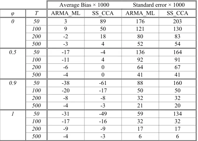
Table 1. Average bias and standard error for the estimates of φaccording to the ARMA(1,1)_ML and

SS(1)_CCA procedures, calculated in a 1000-replicate series of DGP1 with θ = .9

In Table 1 we show some representative results for the estimation of φwith high values of θ(θ = 0.9). The same information can be graphically seen in Figure 1. Except for T = 50 or φ = 0, the estimates provided by CCA are very close to those provided by ML. However, when T = 50, the CCA estimates show a remarkably greater dispersion than the ML estimates.

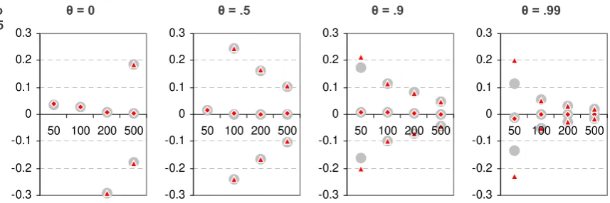
In Figure 2 we can see some representative results for the estimation of the moving-average parameter θ. As the value of θ approaches the unit circle, the estimates provided by CCA show an increasing bias, while the ML estimates do not. The dispersion of the CCA estimates is also higher than that of the ML estimates, especially for low sample sizes.

θ φ = 0 φ = .5 φ = .9 φ = 1

.9

-0.3 -0.2 -0.1 0 0.1 0.2 0.3

50 100 200 500

-0.3 -0.2 -0.1 0 0.1 0.2 0.3

50 100 200 500

-0.3 -0.2 -0.1 0 0.1 0.2 0.3

50 100 200 500

-0.3 -0.2 -0.1 0 0.1 0.2 0.3

50 100 200 500

φ θ = 0 θ = .5 θ = .9 θ = .99 .5 -0.3 -0.2 -0.1 0 0.1 0.2 0.3

50 100 200 500

-0.3 -0.2 -0.1 0 0.1 0.2 0.3

50 100 200 500

-0.3 -0.2 -0.1 0 0.1 0.2 0.3

50 100 200 500

-0.3 -0.2 -0.1 0 0.1 0.2 0.3

50 100 200 500

Figure 2. Average error and +/- 2 standard error bands for the estimation of θ. With φ = .5 and T = {50, 100, 200, 500}. The grey large dots correspond to the ARMA(1,1) prediction-error (ML) estimates and the small red diamonds (average) and triangles (error bands) correspond to the SS(1) CCA estimates. Values out of the range of the figures are not represented.

Note that the different precision in the estimation of the system parameters is not

associated to the different representations (SS or ARMA), but to the different estimation algorithms (ML or CCA). The SS(1) CCA estimates can be further “refined” through a PEM method: the PEM iterative process would begin with the parameter values

provided by CCA. In Figure 3 we can see how the properties of the estimates provided by the SS(1) models are basically the same as those corresponding to the ARMA(1,1) models when the estimation is made using a prediction-error (equivalent to ML) method in both cases. There are still some differences in variability when T = 50, which are probably due to the different algorithms used to find initial estimates of the parameters for the prediction-error search: CCA in the SS case and the default instrumental

variables method of the MATLAB “armax” command in the ARMA case (Ljung 2006).

φ θ = 0 θ = .5 θ = .9 θ = .99

.5 -0.3 -0.2 -0.1 0 0.1 0.2 0.3

50 100 200 500

-0.3 -0.2 -0.1 0 0.1 0.2 0.3

50 100 200 500

-0.3 -0.2 -0.1 0 0.1 0.2 0.3

50 100 200 500

-0.3 -0.2 -0.1 0 0.1 0.2 0.3

50 100 200 500

Figure 3. Average error and +/- 2 standard error bands for the estimation of θ. With φ = .5 and T = {50, 100, 200, 500}. The grey large dots correspond to the ARMA(1,1) prediction-error (ML) estimates and the small red diamonds (average) and triangles (error bands) correspond to the SS(1) prediction-error (ML) estimates, with an initial CCA estimate for the prediction-error search. Values out of the range of the figures are not represented.

φ θ = 0 θ = .5 θ = .9 θ = .99 .5

-1 -0.5 0 0.5 1

50 100 200 500

-1 -0.5 0 0.5 1

50 100 200 500

-1 -0.5 0 0.5 1

50 100 200 500

-1 -0.5 0 0.5 1

50 100 200 500

Figure 4. Average error and +/- 2 standard error bands for the estimation of σ2. With φ = .5 and T = {50, 100, 200, 500}. The grey large dots correspond to the ARMA(1,1) prediction-error (ML) estimates and the small red diamonds (average) and triangles (error bands) correspond to the SS(1) CCA estimates. Values out of the range of the figures are not represented.

θ φ = 0 φ = .5 φ = .9 φ = 1

.9

-1 -0.5 0 0.5 1

50 100 200 500

-1 -0.5 0 0.5 1

50 100 200 500

-1 -0.5 0 0.5 1

50 100 200 500

-1 -0.5 0 0.5 1

50 100 200 500

Figure 5. Average error and +/- 2 standard error bands for the estimation of σ2. With θ = .9 and T = {50, 100, 200, 500}. The grey large dots correspond to the ARMA(1,1) prediction-error (ML) estimates and the small red diamonds (average) and triangles (error bands) correspond to the SS(1) CCA estimates. Values out of the range of the figures are not represented.

In brief, in these experiments, provided that the sample size is 100 or greater, the CCA algorithm we are considering recovers rather well the autoregressive parameter of the ARMA(1,1) model, but not so well the moving-average parameter, especially when its value is close to 1 (close to the unit circle).

3.2.2 Forecasting

Following the indicated methodology, for each considered combination of the values of (φ, θ, T) we generate 1000 time series. Then, for each time series and for each system-identification method we estimate a model and calculate the quality-of-prediction indicator (MSPEmethod) for the one-step ahead prediction error in the last 10 observations

(recalculating the models as the new observations are incorporated in the time series). Then we compare the values MSPEmethod for the different system-identification

methods.

We start by comparing the predictive performance of the AR models estimated by least squares (LS) with the predictive performance of the SS models estimated by the

subspace CCA algorithm. The relative performance of the different methods showed little dependence on the considered values of φ, so here we present representative results corresponding to φ = .9.

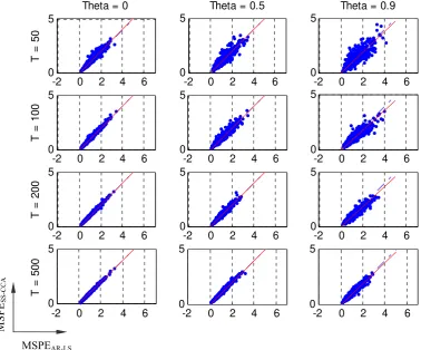
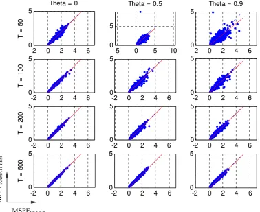
In Figure 6 we show, for different values of T and θ, plots of the associated 1000 points (MSPEAR-LS , MSPESS-CCA). Points below the 45º line (defined by the equation

MSPESS-CCA = MSPEAR-LS) correspond to MSPESS-CCA < MSPEAR-LS, so that the

associated sample was forecasted with less MSPE by the SS-CCA models than by the AR-LS models.

The regression line for a projection of MSPESS-CCA on MSPEAR-LS has also been

-2 0 2 4 6 0

5

Theta = 0

T =

5

0

-2 0 2 4 6

0 5

Theta = 0.5

-2 0 2 4 6

0 5

Theta = 0.9

-2 0 2 4 6

0 5

T =

1

0

0

-2 0 2 4 6

0 5

-2 0 2 4 6

0 5

-2 0 2 4 6

0 5

T =

2

0

0

-2 0 2 4 6

0 5

-2 0 2 4 6

0 5

-2 0 2 4 6

0 5

T =

5

0

0

-2 0 2 4 6

0 5

-2 0 2 4 6

0 5

Figure 6. MSPE of the forecasts of SS-CCA models vs. AR-LS models in a 1000-replicate series of

DGP1 with φ = .9

θ

T 0 0.5 0.9

50 1.02 1.01 0.94

100 1.01 0.99 0.90

200 1.00 1.00 0.92

500 1.00 1.00 0.95

Table 2. Slopesof the regressions of MSPESS-CCA on MSPEAR-LS calculatedin a 1000-replicate series of

DGP1 with φ = .9

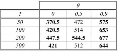
In Table 3 we show the number of samples in which the SS-CCA models “beat” the AR-LS models, calculated as the number of samples satisfying MSPESS-CCA < MSPE AR-LS plus half the number of samples satisfying MSPESS-CCA = MSPEAR-LS .3

With the data in Table 3 we can conduct a binomial statistical test (Siegel and Castellan

3

The incidence of cases MSPEmethod1 = MSPEmethod2 was very low for almost every pair of methods: less

than 5 cases out of 1000 and about 0.1% on average. Only when the methods were SS(1)-ML and ARMA(1,1)-ML would the number of equalities rise remarkably, getting occasionally to even more than 10%.

MSPEAR-LS

MSP

1988; Diebold and Mariano 2002). Using as null hypothesis that the SS-CCA models and the AR-LS models are equally likely to make the best predictions (smaller MSPE) in a sample, i.e. equally likely to “beat” each other in a forecasting tournament, the number of samples in which the SS-CCA models beat the AR-LS models out of a series of N samples should follow a binomial distribution such that the probability of having x

samples in which SS-CCA models beat AR-LS models is

P(x out of N) = _⎟⎟

⎠ ⎞ ⎜⎜ ⎝ ⎛

x N

(½)x (1- ½ )N-x

For a series of 1000 samples we have P(459 ≤x≤ 541) = 0.991, and P(448 ≤x≤ 552) = 0.999. So, for values of x outside the range [459, 541] we can reject (with error α < 0.01) the null hypothesis that both models (AR and CCA) are equally likely to beat each other, and accept that one of the methods is likely to make forecasts with less MSPE than the other.

θ

T 0 0.5 0.9

50 370.5 472 575

100 420.5 514 653

200 447.5 544.5 677

500 421 512 644

Table 3. Number of samples in which MSPESS-CCA < MSPEAR-LS , plus half the number of samples in

which MSPESS-CCA = MSPEAR-LS, out of a 1000-replicate series. Significant values for a binomial test (H0

: P(MSPESS-CCA < MSPEAR-LS) = P(MSPEAR-LS < MSPESS-CCA); α < 0.01, two-sided test) are shown in

bold.

In Table 3 we can see that when the MA component θ is 0, there are significant forecasting differences in favour of the AR-LS models, but when the MA component θ is .9, there are significant forecasting differences in favour of the SS-CCA models, and, in this last case, for sample sizes 100, 200 and 500, the differences are remarkable.

In Table 4 we can see the per cent increase (decrease for negative values) in MSPE of SS-CCA models with respect to AR-LS models. We can use a test for the equality of “prediction accuracy” based on Diebold and Mariano (2002): as each one of the 1000 generated samples is independent of the others, we can assume that the values di =

(MSPESS-CCA - MSPEAR-LS)i , with i = 1, 2, …, 1000, come from i.i.d. variables (this is

for each combination of values of the parameters). Then, to test the null hypothesis E(MSPESS-CCA)i = E(MSPEAR-LS)i or, equivalently, E(di) = 0, we can use the statistic

S =

) ( _i

i

d std

d

N

where N is the number of samples (1000), d_i is the sample average and std(di) is the

approach a standard normal distribution. Significant values for this test with α = 0.01 (|S| > 2.58) are shown in bold in Table 4.

Our results show that, for θ = 0 (when an AR is a right specification), the AR-LS models are likely to improve the forecasts made by the SS-CCA models (Table 3), but both forecasts show in this case a similar MSPE (Figure 6) and there is little global difference between them (Table 4). On the other hand, for θ = 0.9 (now an AR is not a right specification and the MA value is close to the unit circle), the SS-CCA models are likely to improve the forecasts made by the AR-LS models (Table 3), and there are greater differences in MSPE (7% reduction in some cases; Figure 6 and Table 4, right column).

θ

T 0 0.5 0.9

50 2% 3% -3%

100 1% 0% -7%

200 0% 0% -7%

500 0% 0% -4%

θ

T 0 0.5 0.9

50 -6,01 -4,31 3,79

100 -4,95 -0,55 12,00

200 -1,87 -0,35 13,24

500 -2,60 1,00 10,35

Table 4. Left: total increase in MSPESS-CCA with respect to MSPEAR-LS out of a 1000-replicate series of

DGP1 with φ = .9. Right: corresponding values of the statistic S. Significant values (α = 0.01) are shown

in bold.

These results are in favour of using SS-CCA models as an alternative or complement to VAR models for stochastic time series, given that both types of models can be obtained very quickly by non-iterative methods. It would also be interesting to know what can be gained by using other, more involved, estimation methods, or by imposing the right specification for the studied process. We will now try to give an answer to the following questions in relation to our simulated ARMA(1,1) process:

Question 1: How much can be gained by using an ARMA(1,1)-ML model (i.e. the right specification when θ≠ 0) instead of an AR-LS model (specified according to AIC)?

Question 2: How much can be gained by using an ARMA(1,1)-ML model (i.e. the right specification when θ≠ 0) instead of a SS-CCA model?

Question 3: How much can be gained by refining the obtained SS-CCA models through a prediction-error (ML) method?

Question 4: Are there forecasting differences between SS(1)-ML models (i.e. SS models with the right specification and a ML estimation) and ARMA(1,1)-ML models (i.e. ARMA models with the right specification and ML estimation)?

Question 1: How much can be gained by using an ARMA(1,1)-ML model (the right

-2 0 2 4 6 0

5

Theta = 0

T =

5

0

-5 0 5 10

0 5

Theta = 0.5

-2 0 2 4 6

0 5

Theta = 0.9

-2 0 2 4 6

0 5

T =

1

0

0

-2 0 2 4 6

0 5

-2 0 2 4 6

0 5

-2 0 2 4 6

0 2 4

T =

2

0

0

-2 0 2 4 6

0 5

-2 0 2 4 6

0 5

-2 0 2 4 6

0 5

T =

5

0

0

-2 0 2 4 6

0 5

-2 0 2 4 6

0 5

Figure 7. MSPE of the forecasts of ARMA11-ML models vs AR-LS models in a 1000-replicate series of

DGP1 with φ = .9

θ

T 0 0.5 0.9

50 1.01 0.94 0.79

100 1.00 0.96 0.84

200 1.00 0.98 0.89

500 1.00 0.99 0.94

Table 5. Slopesof the regressions of MSPEARMA11-ML on MSPEAR-LS calculatedin a 1000-replicate series

of DGP1 with φ = .9

θ

T 0 0.5 0.9

50 370.5 472 575

100 420.5 514 653

200 447.5 544.5 677

500 421 512 644

Table 6. Number of samples in which MSPEARMA11-ML < MSPEAR-LS , plus half the number of samples in

which MSPEARMA11-ML = MSPEAR-LS, out of a 1000-replicate series. Significant values for an

equal-forecasting-accuracy binomial test (α < 0.01, two-sided test) are shown in bold.

MSPEAR-LS

MSP

EARMA11-P

E

θ

T 0 0.5 0.9

50 1% -5% -17%

100 0% -3% -13%

200 0% -2% -9%

500 0% -1% -5%

θ

T 0 0.5 0.9

50 4,22 -5,04 -18,97

100 1,91 -7,40 -18,46

200 0,78 -6,89 -15,20

500 1,64 -6,51 -12,47

Table 7. Left: total increase in MSPEARMA11-ML with respect to MSPEAR-LS out of a 1000-replicate series

of DGP1 with φ = .9. Right: corresponding values of the statistic S. Significant values (α = 0.01) are

shown in bold.

Our results show that, for θ = 0 (when an AR is a right specification), the AR-LS models are likely to improve the forecasts made by the ARMA(1,1)-ML models (Table 6), but the differences in MSPE are then small (Table 7). For every other case there is an advantage of the ARMA(1,1)-ML models over the AR-LS models (Figure 5, Table 5). This advantage grows with θ (within the considered values) and can get very remarkable for θ = 0.9. The advantage of ARMA(1,1)-ML over AR-LS also seems to decrease as the sample size grows.

Question 2: How much can be gained by using an ARMA(1,1)-ML model (the right

specification when θ≠ 0) instead of a SS-CCA model?

-2 0 2 4 6

0 5

Theta = 0

T =

5

0

-5 0 5 10

0 5

Theta = 0.5

-2 0 2 4 6

0 5

Theta = 0.9

-2 0 2 4 6

0 5 T = 1 0 0

-2 0 2 4 6

0 5

-2 0 2 4 6

0 5

-2 0 2 4 6

0 5 T = 2 0 0

-2 0 2 4 6

0 5

-2 0 2 4 6

0 5

-2 0 2 4 6

0 5 T = 5 0 0

-2 0 2 4 6

0 5

-2 0 2 4 6

0 5

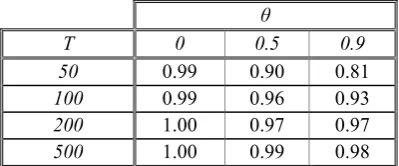
Figure 8. MSPE of the forecasts of ARMA11-ML models vs SS-CCA models in a 1000-replicate series

of DGP1 with φ = .9

MSPESS-CCA

MSP

EARMA11-P

E

θ

T 0 0.5 0.9

50 0.99 0.90 0.81

100 0.99 0.96 0.93

200 1.00 0.97 0.97

500 1.00 0.99 0.98

Table 8. Slopesof the regressions of MSPEARMA11-ML on MSPESS-CCA calculatedin a 1000-replicate series

of DGP1 with φ = .9

θ

T 0 0.5 0.9

50 495 641 740

100 496.5 574 657

200 508 597.5 595

500 485.5 567 576

Table 9. Number of samples in which MSPEARMA11-ML < MSPESS-CCA , plus half the number of samples in

which MSPEARMA11-ML = MSPESS-CCA, out of a 1000-replicate series of DGP1 with φ = .9. Significant

values for a binomial test (H0 : P(MSPEARMA11-ML < MSPESS-CCA) = P(MSPEARMA11-ML > MSPESS-CCA); α

< 0.01, two-sided test) are shown in bold.

θ

T 0 0.5 0.9

50 -1% -7% -14%

100 -1% -3% -6%

200 0% -2% -2%

500 0% -1% -1%

θ

T 0 0.5 0.9

50 -2,42 -7,30 -14,93

100 -3,63 -7,14 -10,96

200 -1,32 -6,98 -6,25

500 -1,59 -5,73 -5,28

Table 10. Left: total increase in MSPEARMA11-ML with respect to MSPESS-CCA out of a 1000-replicate series

of DGP1 with φ = .9. Right: corresponding values of the statistic S. Significant values (α = 0.01) are

shown in bold.

We find that, but for θ = 0, the ARMA(1,1)-ML models are likely to improve the forecasts made by the SS-CCA models (Table 9). The advantage of ARMA(1,1)-ML over SS-CCA decreases as the sample size grows (Table 8 and Table 10). The greatest reductions in MSPEARMA11-ML with respect to MSPESS-CCAare obtained for small sample

sizes (T = 50) and for θ = .9 (Table 10). Note that, when θ = .9 (large MA component), the reductions in MSPE obtained by ARMA(1,1)-ML models compared to SS-CCA models (Table 10) are not as large as when compared to AR-LS models (Table 7).

Question 3: How much can be gained by refining the obtained SS-CCA models through

a prediction-error (maximum likelihood) method?

numerical search for the parameter values that minimise the sample likelihood function (Gaussian innovations).

-2 0 2 4 6

0 5

Theta = 0

T =

5

0

-2 0 2 4 6

0 5

Theta = 0.5

-2 0 2 4 6

0 5

Theta = 0.9

-2 0 2 4 6

0 5

T =

1

0

0

-2 0 2 4 6

0 5

-2 0 2 4 6

0 5

-2 0 2 4 6

0 5

T =

2

0

0

-2 0 2 4 6

0 5

-2 0 2 4 6

0 5

-2 0 2 4 6

0 5

T =

5

0

0

-2 0 2 4 6

0 5

-2 0 2 4 6

0 5

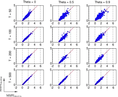
Figure 9. MSPE of the forecasts of SS-ML models vs SS-CCA models in a 1000-replicate series of

DGP1 with φ = .9

θ

T 0 0.5 0.9

50 1.00 0.96 0.94

100 0.99 0.98 0.97

200 1.00 0.98 0.98

500 1.00 0.99 0.99

Table 11. Slopesof the regressions of MSPESS-ML on MSPESS-CCA calculatedin a 1000-replicate series of

DGP1 with φ = .9

MSPESS-CCA

MSP

θ

T 0 0.5 0.9

50 487 557 592

100 485 550 583

200 510.5 579 576

500 479 566 563

Table 12. Number of samples in which MSPESS-ML < MSPESS-CCA , plus half the number of samples in

which MSPESS-ML = MSPESS-CCA, out of a 1000-replicate series of DGP1 with φ = .9. Significant values

for a binomial test (H0 : P(MSPESS-ML < MSPESS-CCA) = P(MSPESS-ML > MSPESS-CCA); α < 0.01, two-sided

test) are shown in bold.

θ

T 0 0.5 0.9

50 0% -3% -4%

100 -1% -2% -2%

200 0% -2% -1%

500 0% -1% -1%

θ

T 0 0.5 0.9

50 -0,55 -4,64 -4,91

100 -3,14 -3,89 -3,72

200 -0,59 -4,78 -3,05

500 -1,23 -5,61 -2,96

Table 13. Left: total increase in MSPESS-ML with respect to MSPESS-CCA out of a 1000-replicate series of

DGP1 with φ = .9. Right: corresponding values of the statistic S. Significant values (α = 0.01) are shown

in bold.

In brief, refining the CCA estimates through a prediction-error method (which for Gaussian innovations and a quadratic loss function is equivalent to maximum likelihood) will do no harm, and when the MA component θ is not null it is likely to provide forecasts with less MSPE (Table 12). Note however that the gains in MSPE that we obtained are usually moderate (Table 13), especially for large sample sizes (T = 200, 500). The gains in MSPE obtained by ARMA(1,1)-ML models are larger than those obtained by SS-ML models, but note that in the first case we are imposing the right specification, while in the second case the SS-ML models are using the system order estimated by the CCA algorithm (Appendix II).

Question 4: Are there forecasting differences between SS(1)-ML models (SS models

-2 0 2 4 6 0

5

Theta = 0

T =

5

0

-5 0 5 10

0 5

Theta = 0.5

-2 0 2 4 6

0 5

Theta = 0.9

-2 0 2 4 6

0 5

T =

1

0

0

-2 0 2 4 6

0 5

-2 0 2 4 6

0 5

-2 0 2 4 6

0 5

T =

2

0

0

-2 0 2 4 6

0 5

-2 0 2 4 6

0 5

-2 0 2 4 6

0 5

T =

5

0

0

-2 0 2 4 6

0 5

-2 0 2 4 6

0 5

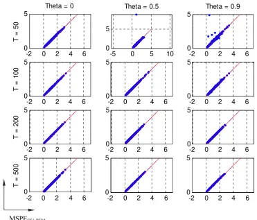
Figure 10. MSPE of the forecasts of ARMA11-ML models vs SS1-ML models in a 1000-replicate series

of DGP1 with φ = .9

θ

T 0 0.5 0.9

50 1.00 1.01 1.00

100 1.00 1.00 1.00

200 1.00 1.00 1.00

500 1.00 1.00 1.00

Table 14. Slopesof the regressions of MSPEARMA11-ML on MSPESS1-ML calculatedin a 1000-replicate

series of DGP1 with φ = .9

θ

T 0 0.5 0.9

50 505 489 484.5

100 496.5 507.5 518

200 491 507 487.5

500 475.5 485.5 488

Table 15. Number of samples in which MSPEARMA11-ML < MSPESS1-ML , plus half the number of samples

in which MSPEARMA11-ML = MSPESS1-ML, out of a 1000-replicate series of DGP1 with φ = .9. Significant

values for a binomial test (H0 : P(MSPEARMA11-ML < MSPESS1-ML) = P(MSPEARMA11-ML > MSPESS1-ML); α

< 0.01, two-sided test) are shown in bold. MSPESS1-PEM

MSP

EARMA11-P

E

θ

T 0 0.5 0.9

50 0% 1% 1%

100 0% 0% 0%

200 0% 0% 0%

500 0% 0% 0%

θ

T 0 0.5 0.9

50 0,40 0,97 1,37

100 1,06 -0,30 0,59

200 -0,07 -0,16 -0,95

500 0,62 0,14 -0,93

Table 16. Left: total increase in MSPEARMA11-ML with respect to MSPESS1-ML out of a 1000-replicate series

of DGP1 with φ = .9. Right: corresponding values of the statistic S. Significant values (α = 0.01) are

shown in bold.

The MSPE provided by SS(1)-ML and ARMA(1,1)-ML models is basically the same, as can be checked graphically on Figure 10 (note the concentration of points around the 45º line) and on the associated tables (Table 14, Table 15 and Table 16).

Summary of results for DGP1

To summarize the results of our simulations with the univariate ARMA(1,1) process DGP1:

- The CCA state space models provided better forecasts than the AR models when the MA component was large (θ = .9) (see rightmost column of Table 2, Table 3 and Table 4).

- For a large MA component (θ = .9), a correct ARMA(1,1) specification would reduce considerably and significantly the MSPE of the AR approximations (see rightmost column of Table 6 and Table 7). It would also reduce considerably and significantly the MSPE of the CCA models (Table 9 and Table 10).

- There was margin to improve the CCA models through a PEM (maximum

likelihood) method. The reductions in MSPE obtained by the refined models were in general statistically significant (Table 12 and Table 13), though moderate (less than 5 % reduction in MSPE).

- When the right specification was imposed, both the SS(1) and ARMA(1,1) models estimated by PEM (maximum likelihood) provided basically the same predictive performance.

3.3 Data Generating Process 2

Data generating process 2 (DGP2) is a bivariate cointegrated process defined by the following equations:

y2,t = γ + βy1,t + (1 + θ2 L) e2,t

where L is the lag operator and [e1,te2,t]’ is Gaussian white noise N (0, Ω) with

⎥ ⎦ ⎤ ⎢ ⎣ ⎡ = Ω 1 2 ρσ ρσ σ

DGP2 admits the following VARMA formulation (including the constant term γ):

⎥ ⎦ ⎤ ⎢ ⎣ ⎡ ⎥ ⎦ ⎤ ⎢ ⎣ ⎡ − + ⎥ ⎦ ⎤ ⎢ ⎣ ⎡ + ⎥ ⎦ ⎤ ⎢ ⎣ ⎡ = ⎥ ⎦ ⎤ ⎢ ⎣ ⎡ ⎥ ⎦ ⎤ ⎢ ⎣ ⎡ − ⎥ ⎦ ⎤ ⎢ ⎣ ⎡ − − − − 1 , 2 1 , 1 2 2 1 1 , 2 , 1 1 , 2 1 , 1 , 2 , 1 ) ( 0 0 0 0 1 t t t t t t t t u u u u y y y y θ θ θ β θ γ β

where _⎥

⎦ ⎤ ⎢ ⎣ ⎡ ⎥ ⎦ ⎤ ⎢ ⎣ ⎡ = ⎥ ⎦ ⎤ ⎢ ⎣ ⎡ t t t t e e u u , 2 , 1 , 2 , 1 1 0 1 β

Searching for a variety of statistical properties in the generated processes we selected the parameter space θ1 = {.5, .9} ; θ2 = {.5, .9} ; β = 1 ; ρ = {0, .8} ; σ = {1, 2}; γ = 50. For different sample sizes T = {100, 200, 400, 800} and for every combination of the values (T, θ1, θ2, β, φ, σ), we generate 1000 samples from which we obtain (1000 pairs of) results for the one-step-ahead quality of prediction indicators (MSPEVAR,

MSPECCA), measured for 10 new observations of every sample and recalculating the

models as the new observations are included.

Note that for DGP2 the cointegrating relation is

y2,t - βy1,t = γ + (1 + θ2 L) e2,t

so there is a constant term (γ) in the cointegrating relation.

The VAR or vector error-correction (VEC) models are calculated by Johansen’s procedure adapted for the case of constant terms in the cointegrating relations and no deterministic trends, as described in Appendix I. The correct number of stochastic common trends (i.e. one) has been imposed for Johansen’s models.

For the subspace models, we start by eliminating the effect of the constant term γ, centring the data (subtracting the average values); thus, the following relation is obtained:

(y2,t - y2,T ) - β (y1,t - y1,T ) = e2,t + θ2e2,t-1 – (e2,T + θ2 e2,T−1 )

where xT stands for the sample average of variable x up to time T.

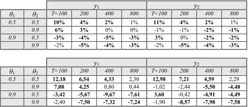
significant advantages of the CCA models over the VEC models are obtained for

sample sizes greater than 100 and for θ1 = .9. In the case of y2,t, significant advantages of

the CCA models over the VEC models are obtained for sample sizes greater than 100 and for (θ2 = .9, σ = 1 ) or (θ1 = .9, σ = 2). On the other hand, significant advantages of the VEC models over the CCA models are usually obtained when forecasting with sample size 100 or 200 and using the small values of θj.

0 2 4 0

2 4

T = 100

T h et a1 = 0 .5 T h et a2 = 0 .5

0 2 4 0 2 4 T he ta1 = 0. 5 T he ta2 = 0. 9

0 2 4 0 2 4 T h et a1 = 0. 9 T h et a2 = 0. 5

0 2 4 0 2 4 T h et a1 = 0. 9 T h et a2 = 0. 9

0 1 2 3 0

1 2 3

T = 200

0 1 2 3 0

1 2 3

0 2 4 0

2 4

0 1 2 3 0

1 2 3

0 1 2 3 0

1 2 3

T = 400

0 2 4 0

2 4

0 2 4 0

2 4

0 1 2 3 0

1 2 3

0 1 2 3 0

1 2 3

T = 800

0 1 2 3 0

1 2 3

0 1 2 3 0

1 2 3

0 1 2 3 0

1 2 3

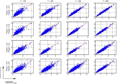
Figure 11. MSPECCA and MSPEVEC for y1,t in a 1000-replicate series of DGP2 with σ = 1 and ρ = .8.

y1 y2

θ1 θ2 T=100 200 400 800 T=100 200 400 800

0.5 0.5 359 441 454 482 345 434 458 468

0.9 436 452 498 511.5 548 519.5 571 565

0.9 0.5 549 578 618 591 441 524 551 572

0.9 539.5 605 607 598 539 625 607 609

Table 17. Number of samples in which MSPECCA < MSPEVEC , plus half the number of samples in which

MSPECCA = MSPEVEC, out of a 1000-replicate series of DGP2 with β = 1, σ = 1 and ρ = .8. Significant

values for a binomial test (H0 : P(MSPECCA < MSPEVEC) = P(MSPECCA > MSPEVEC); α = 0.01, two-sided

test) are shown in bold.

MSPEVEC

MSP

y1 y2

θ1 θ2 T=100 200 400 800 T=100 200 400 800

0.5 0.5 10% 4% 2% 1% 11% 4% 2% 1%

0.9 6% 3% 0% 0% -1% -1% -2% -1%

0.9 0.5 -3% -4% -5% -3% 3% 0% -2% -2%

0.9 -2% -5% -4% -3% -2% -5% -4% -3%

y1 y2

θ1 θ2 T=100 200 400 800 T=100 200 400 800

0.5 0.5 12,18 6,54 4,33 2,30 12,98 7,21 4,59 2,29

0.9 7,08 4,25 0,80 0,44 -1,02 -2,44 -5,50 -4,48

0.9 0.5 -3,42 -5,67 -9,67 -7,61 3,60 -0,42 -4,91 -4,49

0.9 -2,40 -7,50 -7,32 -7,24 -1,90 -8,57 -7,98 -7,58

Table 18. Top table: total increase in MSPECCA with respect to MSPEVEC out of a 1000-replicate series of

DGP2 with β = 1, σ = 1 and ρ = .8. Bottom table: corresponding values of the statistic S. Significant

values (α = 0.01) are shown in bold.

Table 19 shows some results corresponding to the Adapted Canonical Correlation Analysis (ACCA) models of Bauer and Wagner (2002). Although, within the considered algorithms, consistent estimation of all system parameters of VARMA cointegrated systems has only been proven for the ACCA algorithm, in our simulations, the ACCA models did not show predictive advantages over the CCA models (the ACCA models showed similar performance to the CCA models; they were better in some occasions but worse in some others).

Augmenting the prediction horizon usually involves gradual little changes in the tournament results. In general, as in Bauer and Wagner (2003), we found a relative improvement in the performance of Johansen’s model as the prediction horizon grows, probably because this model imposes a value of exactly 1 for the non stationary roots (which is the right value for our simulated processes). However, the unit root

restrictions can also be considered in the subspace model through a reduced-rank regression in the estimation of the state transition matrix (Reinsel and Velu 1998; Bauer and Wagner 2002), imposing that the rank of (A - In ) must be (n - c), where n is the

y1 y2

θ1 θ2 T=100 200 400 800 T=100 200 400 800

0.5 0.5 16% 7% 3% 1% 5% 3% 2% 1%

0.9 27% 18% 12% 7% 4% 2% 1% 0%

0.9 0.5 26% 16% 8% 5% 7% 4% 1% 1%

0.9 24% 15% 10% 7% 3% 0% 0% 0%

y1 y2

θ1 θ2 T=100 200 400 800 T=100 200 400 800

0.5 0.5 15,45 11,30 7,84 5,25 8,30 7,53 5,64 3,16

0.9 20,26 19,39 17,49 13,00 5,12 4,13 2,51 0,79

0.9 0.5 18,48 16,10 11,77 9,33 9,60 6,81 3,34 1,87

0.9 16,48 14,84 13,32 11,73 3,61 -0,43 -0,20 -0,68

Table 19. Top table: total increase in MSPEACCA with respect to MSPEVEC out of a 1000-replicate series

of DGP2 with β = 1, σ = 1 and ρ = .8. Bottom table: corresponding values of the statistic S. Significant

values (α = 0.01) are shown in bold.

Summary of results for DGP2

DGP2 is a VARMA bivariate cointegrated process used to compare the forecasting accuracy of Johansen’s VEC models with that of SS CCA models. Our results show that the MA components have a large influence on the relative finite-sample performance of both methods. In our experiments, large values (close to 1) of the MA components usually led to relative advantages for the SS CCA models.

4. A practical case

In this section we compare, for two cointegrated series of real data, the point and density forecasts made by CCA models with those made by Johansen’s VAR models.

We take a series of 4,805 crude oil daily prices between January 1986 and March 2005, as well as the corresponding “oil future contract” prices. The data is freely provided by the U.S. Energy Information Administration in their web page. The spot prices

correspond to “Cushing, OK WTI Spot Price FOB ($/bbl)” and the future prices to “Cushing, Ok Crude Oil Future Contract 4 ($/bbl)”. Instead of working directly with prices, whose variations have a lower bound and are expected to be proportional to the price level, we take the logarithms of the original data: y1= log(spot), y2= log(future).

Jan 19862.2 March 2005 2.4

2.6 2.8 3 3.2 3.4 3.6 3.8 4 4.2

Figure 12. The studied sample: log(spot) and log(future).

The autocorrelogram and partial autocorrelogram for the series log(spot) and log(future)

are shown in Figure 13.

0 10 20 30

-0.5 0 0.5 1

Au

to

c

o

rr

e

la

ti

o

n

log(spot)

0 10 20 30

-0.5 0 0.5 1

log(future)

0 10 20 30

-0.5 0 0.5 1

Lag

P

a

rt

ia

l A

u

to

c

o

rrel

a

ti

o

n

s log(spot)

0 10 20 30

-0.5 0 0.5 1

Lag log(future)

Figure 13. Autocorrelogram and partial autocorrelogram for the series log(spot)-left- and log(future)-right-.