A Simulated Annealing approach for solving Minimum
Manhattan Network Problem
S. M. Ferdous
Ahsanullah University of Science and Technology(AUST) Dhaka
Anindya Das
Iowa State University, AmesIowa
ABSTRACT
In this paper we address the Minimum Manhattan Network (MMN) problem. It is an important geometric problem with vast applications. As it is an NP-complete discrete combina-torial optimization problem we employ a simple metaheuris-tic namely Simulated Annealing. We have also developed benchmark datasets and tested our algorithm with the dataset.
General Terms:
Experimental Algorithms, Stochastic Approach
Keywords:
Combinatorial Optimization, Metaheuristics, Simulated Anneal-ing, Network Length
1. INTRODUCTION
Finding minimum network length is an important problem in com-puter science. In this paper we address the problem of finding minimum network length inManhattanmetric. Given two points p, q∈R2, arectilinear pathis achieved between these two points if all the line segments along the path is either vertical or horizontal. To a find aManhattanpath betweenpandqtwo properties must be satisfied:
—The path betweenpandqmust berectilinear.
—The length of the path is exactly equals todist(p, q) =kp.x− q.xk+kp.y−q.yk.
In MMN problem, we are given a setT ofnpoints inR2. A
net-workMis said to be manhattan network onT, if for allp, q∈T, there exist at least one Manhattan path betweenpandqwith all its edge segment onM. Minimum Manhattan Network problem is to find the Manhattan NetworkMwith minimum network length.
MMN has vast applications in geometric network design as well as in VLSI circuit design, where the (rectilinear) characteristics of Manhattan networks adapt well to reality. An important example is computer chip manufacturing where all the circuit paths are usually rectilinear paths. Furthermore, the MMN problem has its applica-tions in city planning, network layout and distributed algorithms [9].
MMN has its application in the field of computational biology. In [14], the author present a solution to the problem of designing effi-cient search spaces for pair hidden Markov models that align bio-logical sequences using Manhattan networks.
2. LITERATURE REVIEW
The MMN problem has various applications already discussed in the previous section. Therefore, researchers started to work with this problem. Gudmundsson et al. [8] first published anO(n3)time
4-approximation algorithm. Moreover, they proposed anO(nlgn) time8-approximation algorithm and also discussed the problem of determining the complexity class of this problem.
Gudmundsson et al. [8] conjectured that there could be a 2-approximation algorithm. Kato et al. [11] proved them right by pro-viding anO(n3)time2-approximation algorithm, although using
a different approach. The key idea provided by them is to deter-mine efficiently whether a graph is a Manhattan Network or not. A naive approach is to check whether Manhattan path exists for all O(n2)pairs of nodes, but they proved that it is sufficient to
check onlyO(n)specific pair of points. Using similar idea as [11], Benkert et al. [1] proposed a3-approximation algorithm which runs inO(nlgn)time and takes linear space.
Benkert et al. [2] also proposed a mixed integer programming for-mulation. Chepoi et al. [4] used the idea of Pareto front and strip-staircase decomposition to derive a rounding2-approximation al-gorithm based on an LP-formulation of the problem. Later, Guo et al. [9] proposed a2-approximation algorithm based on dynamic programming which runs inO(n2)time. They also proposed
an-other approximation algorithm with same approximation ratio, but with a better running time ofO(nlgn)using a simple greedy strat-egy [10]. Seibert et al. [15] provided a1.5-approximation algo-rithm.
First approximation algorithm for Generalized Minimum Manhat-tan Network was proposed by Das et al. [6]. For an arbitrary di-mensiond, they proposed an algorithm with approximation ratio O(lgd+1n).
3. BASICS OF SIMULATED ANNEALING (SA)
Simulated Annealing (SA) is a generic probabilistic algorithm and it is sometimes commonly said to be the oldest among the meta-heuristics. It is also one of the first algorithms that had an explicit strategy to escape from local minima. The name and inspiration come from annealing in metallurgy, a technique that involve heat-ing and controlled coolheat-ing of a material. Heatheat-ing and coolheat-ing the material affects both the temperature and the thermodynamic free energy. While the same amount of cooling brings the same amount of decrease in temperature it will bring a bigger or smaller decrease in the thermodynamic free energy depending on the rate that it oc-curs, with a slower rate producing a bigger decrease.
This notion of slow cooling is implemented in the Simulated An-nealing algorithm as a slow decrease in the probability of accepting worse solutions as it explores the solution space. SA was first pre-sented as a search algorithm for Combinatorial Optimization prob-lems in [7, 12] . The basic idea is to permit moves that result in solutions of worse quality than the current solution (uphill moves) to escape from local minima. The probability of doing such a move is decreased during the search which is controlled by the tempera-ture parameter. The high level algorithm is described in Algorithm (1).
Algorithm 1Generic SA [3]
s←GenerateInitialSolution() T ←T0
whiletermination condition not metdo
s0←PickAtRandom(Neighbor(s))
iff(s)< f(s0) then
s←s0 else
Accepts0
as new solution with probabilityp(T, s0, s) end if
Update(T)
end while
4. OUR APPROACH: SIMULATED ANNEALING FOR MMN
In this section, we will describe the SA implementation for MMN in details. The high-level pseudocode for solving MMN by SA is shown in Algorithm (2).
The algorithm starts with initializing a set of parameters. After reading the dataset it starts with generating an initial solution(s). Then at each iteration it selects a new solution(s0) by tweaking the previous one and it is accepted as new current solution depending onsize(s),size(s0)andT wheresize(S)is the fitness(the man-hattan network size) of solutionSandTis the temperature param-eter. As it is described in [3], we will use the Boltzman distribution computed asexp−(size(s
0)−size(s))
T to find the probability of
select-ing a worse solution (p(T, s0, s)). The temperate,T is decreased at each iteration using the equationTi=α×Ti−1, whereα∈[0,1].
Algorithm 2MMNSA
Initializer,c,itLimit,T,α. Read Dataset
manP aths←GENERATESOLUTION(n,m,nN odes)
whileitCounter < itLimitdo
newM anP ath←TWEAK(manP aths)
ifsize(newM anP aths)< size(manP aths)then
manP aths←newM anP aths
else
manP aths ← newM anP aths with probability p(T, manP aths, newM anP aths)
end if
T←α×T
end while
4.1 Generating a solution
For each pair of nodes in the grid, we construct a probabilistic man-hattan path. The manman-hattan network is constructed from all the in-dividual manhattan paths.
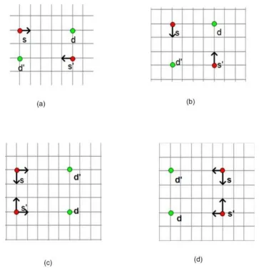
We have developed a stochastic approach to construct a manhattan path between two nodes which will be called source and destination nodes henceforth. The algorithm is iterative in nature. Starting from the source node at each step the algorithm chooses afeasible grid edgerandomly from a uniform distribution. Then the source node is updated to the other end of the chosen edge. The procedure is continued until the source becomes destination. From a source node it is necessary to detect the feasible grid edges. Thefeasible set of edgesfrom a particular source node depend on the orientation of the source and destination nodes. The possible orientation and the feasible edgesare shown in Figure (1). The detailed pseudocode of generating a solution is shown in Algorithm (3)
Algorithm 3Generate a Solution
functionGENERATESOLUTION(r,c,nN odes)
manP ath←a vector of edges manP aths←a vector ofmanP ath
foreach pair of nodes(x, y)and(x0, y0)do
source←(x, y) destination←(x0, y0)
manP ath ← CONSTRUCTMAN
-PATH(source,destination) add(manpaths,manpath)
end for
returnmanP aths
end function
functionCONSTRUCTMANPATH(source,destination)
manP ath←φ
whilesource6=destinationdo
E←feasible grid edges fromsource. e←randomly select an edge fromE. source←Other end point of e. manP ath←append(manPath,e)
end while
returnmanP ath
end function
Fig. 1. Feasible grid edges for different source and destination orientation ((s,d) and (s’,d’)). The bold arrows are the allowed edges from the source node. (a)-(b): Orientations where one edge is feasible. (c)-(d): Orientations where two edges are feasible.
4.2 Tweaking a solution
Tweaking is the process of generating new solutions given any valid solution. To get a new solution we randomly select a pair of nodes. Then we reconstruct the manhattan path between these two nodes. The detailed pseudocode is given in Algorithm (4).
Algorithm 4Tweak a Solution
functionTWEAKSOLUTION(oldM anP ath)
a, b←random2points from the nodes newM anP ath←CONSTRUCTMANPATH(a,b)
newM anP aths←update(oldM anP aths,newM anP ath)
end function
5. EXPERIMENTS
We have conducted our experiments in a computer with Intel Core 2Quad CPU2.33GHz. The available RAM was 4.00GB. The
operating system was Windows7. The programming environment was Matlab.
5.1 Datasets
To our best knowledge, there are not any benchmark dataset for MMN. Here we introduced a random set of data. We set the grid size (r×c) as20×20, i.e. both the number of rows and columns are20. We divide the datasets into four groups. Each group contain 10test cases. Forgroup1each test case contain10points.25,50 and 100points are considered in the each test cases ofgroup2, group3andgroup4respectively.
5.2 Results
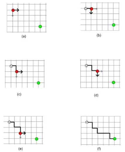
Fig. 2. Generating a solution. (a): feasible grid edges (arrowed) from the source node. Bold arrow is the selected edge. (b): update source according the selected grid edge. (c) - (e): continue selection of feasible grid edges and updating source. (f): Final Manhattan Path
6. CONCLUSION
In this paper we have developed a metaheuristic technique namely Simulated Annealing for solving the MMN problem. We have also developed several benchmark data sets. With these we have re-ported our findings and results. Future research might be in
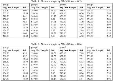
Table 1. Network length by MMNSA (α= 0.2)
group1 group2 group3 group4
Avg. Net. Length Std Avg. Net. Length Std Avg. Net. Length Std Avg. Net. Length Std
201.80 9.04 543.60 18.22 638.30 8.04 758.20 1.32
205.60 15.58 556.50 7.82 661.10 6.76 756.50 2.80
210.50 9.41 563.40 11.77 650.20 9.84 753.10 2.18
251.10 9.87 552.10 8.27 705.50 6.55 754.80 2.86
304.20 7.64 516.20 14.86 739.40 4.30 752.00 3.23
205.10 10.95 523.50 17.60 724.90 6.98 748.60 2.99
216.80 11.73 515.20 13.93 699.70 4.50 739.40 5.02
174.20 11.55 479.30 7.62 712.40 7.09 753.20 2.53
210.70 6.60 442.10 10.20 718.10 5.43 756.20 1.93
228.00 11.43 542.80 7.98 679.90 6.90 753.50 2.42
Table 2. Network length by MMNSA (α= 0.5)
group1 group2 group3 group4
Avg. Net. Length Std Avg. Net. Length Std Avg. Net. Length Std Avg. Net. Length Std
200.30 8.35 538.60 10.30 635.10 7.88 757.80 1.23
206.60 8.37 552.30 10.57 657.50 7.71 755.90 3.11
205.90 12.65 554.50 12.89 654.30 7.51 753.20 2.30
256.40 13.79 554.50 14.52 707.40 6.13 756.30 1.34
307.00 7.83 519.40 13.72 738.50 3.57 753.00 2.83
194.50 9.74 515.80 14.95 721.30 7.56 750.10 3.98
208.20 5.71 514.20 9.80 698.80 6.01 738.70 4.27
164.80 11.09 477.50 7.95 713.40 8.26 752.40 2.95
208.50 4.40 439.50 14.28 718.60 5.58 756.30 1.16
224.80 13.89 537.80 10.14 679.50 5.91 752.60 2.95
7. REFERENCES
[1] Marc Benkert, Alexander Wolff, and Florian Widmann. The minimum manhattan network problem: A fast factor-3 ap-proximation. InProceedings of the 2004 Japanese Confer-ence on Discrete and Computational Geometry, JCDCG’04, pages 16–28, Berlin, Heidelberg, 2005. Springer-Verlag. [2] Marc Benkert, Alexander Wolff, Florian Widmann, and
Takeshi Shirabe. The minimum manhattan network problem: Approximations and exact solutions.Comput. Geom. Theory Appl., 35(3):188–208, October 2006.
[3] Christian Blum and Andrea Roli. Metaheuristics in combi-natorial optimization: Overview and conceptual comparison. ACM Comput. Surv., 35(3):268–308, September 2003. [4] Victor Chepoi, Karim Nouioua, and Yann Vax`es. A rounding
algorithm for approximating minimum manhattan networks. Theor. Comput. Sci., 390(1):56–69, January 2008.
[5] Francis Y.L. Chin, Zeyu Guo, and He Sun. Minimum man-hattan network is np-complete. InProceedings of the Twenty-fifth Annual Symposium on Computational Geometry, SCG ’09, pages 393–402, New York, NY, USA, 2009. ACM. [6] Aparna Das, Krzysztof Fleszar, Stephen G. Kobourov,
Joachim Spoerhase, Sankar Veeramoni, and Alexander Wolff. Polylogarithmic approximation for generalized minimum manhattan networks.CoRR, 2012.
[7] V. ern. Thermodynamical approach to the traveling salesman problem: An efficient simulation algorithm.Journal of Opti-mization Theory and Applications, 45(1):41–51, 1985. [8] Joachim Gudmundsson, Christos Levcopoulos, and Giri
Narasimhan. Approximating a minimum manhattan network. Nordic J. of Computing, 8(2):219–232, June 2001.
[9] Zeyu Guo, He Sun, and Hong Zhu. A fast 2-approximation algorithm for the minimum manhattan network problem. In Rudolf Fleischer and Jinhui Xu, editors,Algorithmic Aspects in Information and Management, volume 5034 of Lecture Notes in Computer Science, pages 212–223. Springer Berlin Heidelberg, 2008.
[10] Zeyu Guo, He Sun, and Hong Zhu. Greedy construction of 2-approximation minimum manhattan network. InProceedings of the 19th International Symposium on Algorithms and Com-putation, ISAAC ’08, pages 4–15, Berlin, Heidelberg, 2008. Springer-Verlag.
[11] Ryo Kato, Keiko Imai, and Takao Asano. An improved algo-rithm for the minimum manhattan network problem. In Pro-ceedings of the 13th International Symposium on Algorithms and Computation, ISAAC ’02, pages 344–356, London, UK, UK, 2002. Springer-Verlag.
[12] S. Kirkpatrick, C. D. Gelatt, and M. P. Vecchi. Optimiza-tion by simulated annealing.SCIENCE, 220(4598):671–680, 1983.
[13] Xavier Muoz, Sebastian Seibert, and Walter Unger. The min-imal manhattan network problem in three dimensions. In Sandip Das and Ryuhei Uehara, editors, WALCOM: Algo-rithms and Computation, volume 5431 ofLecture Notes in Computer Science, pages 369–380. Springer Berlin Heidel-berg, 2009.
[14] Lior Pachter and Fumei Lam. Picking alignments from (steiner) trees. In Proceedings of the Sixth Annual Interna-tional Conference on ComputaInterna-tional Biology, RECOMB ’02, pages 246–253, New York, NY, USA, 2002. ACM.
Table 3. Network length by MMNSA (α= 0.8)
group1 group2 group3 group4
Avg. Net. Length Std Avg. Net. Length Std Avg. Net. Length Std Avg. Net. Length Std
202.50 5.21 539.50 7.72 638.70 9.18 758.40 1.26
210.70 9.74 544.60 9.94 661.30 6.96 757.00 1.70
207.70 17.47 567.10 7.29 650.90 8.18 755.20 2.39
252.70 6.18 548.30 15.31 707.50 1.72 756.60 1.90
304.90 9.95 512.30 13.97 735.60 3.92 754.10 2.60
205.10 10.40 517.70 11.42 725.50 5.21 748.90 2.38
213.00 9.09 512.30 15.04 701.30 4.52 740.50 3.66
175.60 8.09 468.90 12.41 717.00 5.85 753.00 1.56
214.30 11.55 437.20 13.21 714.10 6.40 755.70 2.21
226.90 8.57 539.00 11.37 679.00 8.96 751.60 2.67