Online Adaboost based parameterized methods for dynamic distributed network intrusion detection

BIROn - Birkbeck Institutional Research Online

Weiming, H. and Jun, G. and Yanguo, W. and Ou, W. and Maybank,

Stephen (2014) Online Adaboost-based parameterized methods for dynamic

distributed network intrusion detection. IEEE Transactions on Cybernetics

44 (1), pp. 66-82. ISSN 2168-2267.

Downloaded from:

Usage Guidelines:

Please refer to usage guidelines at or alternatively

Online Adaboost-Based Parameterized Methods for Dynamic

Distributed Network Intrusion Detection

Weiming Hu, Jun Gao, Yanguo Wang, and Ou Wu

(National Laboratory of Pattern Recognition, Institute of Automation, Chinese Academy of Sciences, Beijing 100190) {wmhu, jgao, ygwang, wuou}@nlpr.ia.ac.cn

Stephen Maybank

(Department of Computer Science and Information Systems, Birkbeck College, Malet Street, London WC1E 7HX) [email protected]

Abstract: Current network intrusion detection systems (NIDS) lack the adaptability to the frequently changing

network environments. Furthermore, intrusion detection in the new distributed architectures is now a major

requirement. In this paper, we propose two online Adaboost-based intrusion detection algorithms. In the first

algorithm, a traditional online Adaboost process is used where decision stumps are used as weak classifiers. In

the second algorithm, an improved online Adaboost process is proposed, and online GMMs are used as weak

classifiers. We further propose a distributed intrusion detection framework, in which a local parameterized

detection model is constructed in each node using the online Adaboost algorithm. A global detection model is

constructed in each node by combining the local parametric models using a small number of samples in the node.

This combination is achieved using an algorithm based on particle swarm optimization (PSO) and support vector

machines (SVM). The global model in each node is used to detect intrusions. Experimental results show that the

improved online Adaboost process with GMMs obtains a higher detection rate and a lower false alarm rate than

the traditional online Adaboost process which uses decision stumps. Both the algorithms outperform existing

intrusion detection algorithms. It is also shown that our PSO and SVM-based algorithm effectively combines the

local detection models into the global model in each node: the global model in a node can handle the intrusion

types which are found in other nodes, without sharing the samples of these intrusion types.

Index terms: Network intrusions, Dynamic distributed detection, Online Adaboost learning, Parameterized

model

1. Introduction

Network attack detection is one of the most important problems in network information security. Currently

there are mainly firewall, NIDS/NIPS (network-based intrusion detection and prevention systems) and UTM

(unified threat management) like devices to detect attacks in network infrastructure. NIDS/NIPS detect and

prevent network behaviors which violate or endanger network security. Basically, firewalls are used to block

certain types of traffic to improve the security. NIDS and firewalls can be linked to block network attacks.UTM

devices combine firewall, NIDS/NIPS and other capabilities onto a single device to detect similar events as

standalone firewalls and NIDS/NIPS devices. Deep Packet Inspection (DPI) [52] adds analysis on the application

layer, and then recognizes various applications and their contents. DPI can incorporate NIDS into firewalls. It

can increase the accuracy of intrusion detection, but it is more time-consuming, in contrast to traditional package

header analysis. This paper focuses on investigation of NIDS.

of attacks to detect intrusions by modeling each type of attack. As typical misuse detection methods, pattern

matching methods search packages for the attack features by utilizing protocol rules and string matching. Pattern

matching methods can effectively detect the well-known intrusions. But they rely on the timely generation of

attack signatures, and fail to detect novel and unknown attacks. In the case of rapid proliferation of novel and

unknown attacks, any defense based on signatures of known attacks becomes impossible. Moreover, the

increasing diversity of attacks obstructs modeling signatures.

Machine learning deals with automatically inferring and generalizing dependencies from data to allow

extrapolation of dependencies to unseen data. Machine learning methods for intrusion detection model both

attack data and normal network data, and allow for detection of unknown attacks using the network features [60].

This paper focuses on machine learning-based NIDS. The machine learning-based intrusion detection methods

can be classified as statistics-based, data mining-based, and classification-based. All the three classes of methods

first extract low level features and then learn rules or models which are used to detect intrusions. A brief review

of each class of methods is given below.

1) Statistics-based methods construct statistical models of network connections to determine whether a new

connection is an attack. For instance, Denning [1] construct statistical profiles for normal behaviors. The profiles

are used to detect anomalous behaviors which are treated as attacks. Caberera et al. [2] adopt the Kolmogorov-Smirnov test to compare observation network signals with normal behavior signals, assuming that

the number of observed events in a time segment obeys the Poisson distribution. Li and Manikopoulos [22]

extract several representative parameters of network flows, and model these parameters using a hyperbolic

distribution. Peng et al. [23] use a nonparametric cumulative sum algorithm to analyze the statistics of network data, and further detect anomalies on the network.

2) Data mining-based methods mine rules which are used to determine whether a new connection is an

attack. For instance, Lee et al. [3] characterize normal network behaviors using association rules and frequent episode rules [24]. Deviations from these rules indicate intrusions on the network. Zhang et al. [40] use the random forest algorithm to automatically build patterns of attacks. Otey et al. [4] propose an algorithm for mining frequent itemsets (groups of attribute value pairs) to combine categorical and continuous attributes of

data. The algorithm is extended to handle dynamic and streaming data sets. Zanero and Savaresi [25] first use

unsupervised clustering to reduce the network packet payload to a tractable size, and then a traditional anomaly

detection algorithm is applied to intrusion detection. Mabu et al. [49] detect intrusions by mining fuzzy class association rules using genetic network programming. Panigrahi and Sural [51] detect intrusions using fuzzy

logic, which combines evidence from a user’s current and past behaviors.

3) Classification-based methods construct a classifier which is used to classify new connections as either

attacks or normal connections. For instance, Mukkamala et al. [30] use the support vector machine (SVM) to distinguish between normal network behaviors and attacks, and further identify important features for intrusion

detection. Mill and Inoue [31] propose the TreeSVM and ArraySVM algorithms for reducing the inefficiencies

which arise when a sequential minimal optimization algorithm for intrusion detection is learnt from a large set of

an algorithm for intrusion detection based on the Kohonen self organizing feature map (SOM). Specific attention

is given to a direct labeling of SOM nodes with the connection type. Bivens et al. [26] propose an intrusion detection method in which SOMs are used for data clustering and multi-layer perceptron (MLP) neural networks

are used for detection. Hierarchical neural networks [28], evolutionary neural networks [29], and MLP neural

networks [27], have been applied to distinguish between attacks and normal network behaviors. Hu and

Heywood [6] combine SVM with SOM to detect network intrusions. Khor et al. [55] propose a dichotomization algorithm in which rare categories are separated from the training data and cascaded classifiers are trained to

handle both the rare categories and other categories. Xian et al. [32] combine the fuzzy K-means algorithm with the clonal selection algorithm to detect intrusions. Jiang et al. [33] use an incremental version of the K-means algorithm to detect intrusions. Hoglund et al. [34] extract features describing network behaviors from audit data, and use the SOM to detect intrusions. Sarasamma et al. [18] propose a hierarchical SOM which selects different feature subset combinations that are used in different layers of the SOM to detect intrusions. Song et al. [35] propose a hierarchical random subset selection-dynamic subset selection (RSS-DSS) algorithm to detect

intrusions. Lee et al. [8] propose an adaptive intrusion detection algorithm which combines the adaptive resonance theory with the concept vector and the Mecer-Kernel. Jirapummin et al. [21] employ a hybrid neural network model to detect TCP SYN flooding and port scan attacks. Eskin et al. [20] use a k-nearest neighbor (k-NN)-based algorithm and a SVM-based algorithm to detect anomalies.

Although there is much work on intrusion detection, several issues are still open and require further

research, for example:

 Network environments and the intrusion training data change rapidly over time, as new types of attack

emerge. In addition, the size of the training data increases over time and can become very large. Most

existing algorithms for training intrusion detectors are offline. The intrusion detector must be retrained

periodically in batch mode in order to keep up with the changes in the network. This retraining is time

consuming. Online training is more suitable for dynamic intrusion detectors. New data are used to update

the detector and are then discarded. The key issue in online training is to maintain the accuracy of the

intrusion detector.

 There are various types of attributes for network connection data, including both categorical and

continuous ones, and the value ranges for different attributes differ greatly — from {0, 1} to describe the

normal or error status of a connection, to [0, 107] to specify the number of data bytes sent from source to

destination. The combination of data with different attributes without loss of information is crucial to

maintain the accuracy of intrusion detectors.

 In traditional centralized intrusion detection, in which all the network data are sent to a central site for

processing, the raw data communications occupy considerable network bandwidth. There is a

computational burden in the central site and the privacy of the data obtained from the local nodes cannot

be protected. Distributed detection [36], which shares local intrusion detection models learned in local

nodes, can reduce data communications, distribute the computational burden, and protect privacy. Otey

limitation is that many raw network data still need to be shared among distributed nodes. There is a

requirement for a distributed intrusion detection algorithm to make only a small number of

communications between local nodes.

In this paper, we address the above challenges, and propose a classification-based framework for the

dynamic distributed network intrusion detection using the online Adaboost algorithm [58]. The Adaboost

algorithm is one of the most popular machine learning algorithms. Its theoretical basis is sound, and its

implementation is simple. Moreover, the AdaBoost algorithm corrects the misclassifications made by weak

classifiers and it is less susceptible to over-fitting than most learning algorithms. Recognition performances

of the Adaboost-based classifiers are generally encouraging. In our framework, a hybrid of online weak

classifiers and an online Adaboost process results in a parameterized local model at each node for intrusion

detection. The parametric models for all the nodes are combined into a global intrusion detector in each

node using a small number of samples, and the combination is achieved using an algorithm based on

particle swarm optimization (PSO) and SVMs. The global model in a node can handle the attack types

which are found in other nodes, without sharing the samples of these attack types. Our framework is

original in the following ways:

 In the Adaboost classifier, the weak classifiers are constructed for each individual feature

component, both for continuous and categorical ones, in such a way that the relations between these

features can be naturally handled, without any forced conversions between continuous features and

categorical features.

 New algorithms are designed for local intrusion detection. The traditional online Adaboost process

and a newly proposed online Adaboost process are applied, to construct local intrusion detectors.

The weak classifiers used by the traditional Adaboost process are decision stumps. The new

Adaboost process uses online Gaussian Mixture Models (GMM) as weak classifiers. In both cases

the local intrusion detectors can be updated online. The parameters in the weak classifiers and the

strong classifier construct a parametric local model.

 The local parametric models for intrusion detection are shared between the nodes of the network.

The volume of communications is very small and it is not necessary to share the private raw data

from which the local models are learnt.

 We propose a PSO and SVM-based algorithm for combining the local models into a global detector

in each node. The global detector which obtains information from other nodes obtains more

accurate detection results than the local detector.

The remainder of this paper is organized as follows. Section 2 introduces the distributed intrusion detection

framework. Section 3 describes the online Adaboost-based local intrusion detection models. Section 4 presents

the method for constructing the global detection models. Section 5 shows the experimental results. Section 6

summarizes the paper.

2. Overview of Our Framework

detection model according to its own data. By combining all the local models, at each node, a global model is

trained using a small number of the samples in the node, without sharing any of the original training data

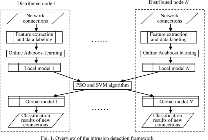
between nodes. The global model is used to detect intrusions at the node. Fig. 1 gives an overview of our

[image:6.595.139.498.140.382.2]

framework which consists of the modules of data preprocessing, local models, and global models.

Fig. 1. Overview of the intrusion detection framework

1) Data preprocessing: For each network connection, three groups of features [9] which are commonly

used for intrusion detection are extracted: basic features of individual TCP (transmission control protocol)

connections, content features within a connection suggested by domain knowledge, and traffic features computed

using a two-second time window [14]. The extracted feature values from a network connection form a vector x = (x1, x2, …, xD), where D is the number of feature components. There are continuous and categorical features,

and the value ranges of the features may differ greatly from each other. The framework for constructing these

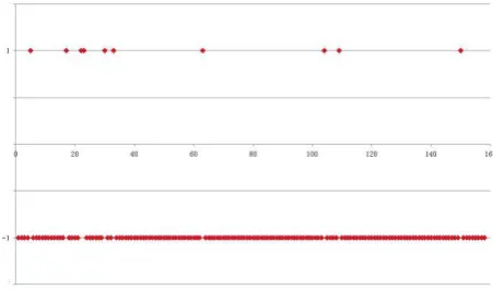
features can be found in [9]. A set of data is labeled for training purposes. There are many types of attacks on the

Internet. The attack samples are labeled as “-1”, “-2”, ... depending on the attack type, and the normal samples

are all labeled as “+1”.

2) Local models: The construction of a local detection model at each node includes the design of weak

classifiers and Adaboost-based training. Each individual feature component corresponds to a weak classifier. In

this way, the mixed attribute data for the network connections can be handled naturally, and full use can be made

of the information in each feature. The Adaboost training is implemented using only the local training samples at

each node. After training, each node contains a parametric model which consists of the parameters of the weak

classifiers and the ensemble weights.

3) Global models: By sharing all the local parametric models, a global model is constructed using the PSO

and SVM-based algorithm in each node. The global model in each node fuses the information learned from all

the local nodes using a small number of training samples in the node. Feature vectors of new network

connections to the node are input to the global classifier, and classified as either normal or attacks. The results of

the global model in the node are used to update the local model in the node and the updated model is then shared

Online Adaboost learning

Local model 1 Network connections

Classification results of new connections

Global model 1 Feature extraction

and data labeling

Distributed node 1 Distributed node N

Online Adaboost learning

Local model N

Network connections

Global model N

Feature extraction and data labeling

Classification results of new connections

……

……

by other nodes.

3. Local Detection Models

The classical Adaboost algorithm [37] carries out the training task in batch mode. A number of weak

classifiers are constructed using a training set. Weights, which indicate the importance of the training samples,

are derived from the classification errors of the weak classifiers. The final strong classifier is an ensemble of

weak classifiers. The classification error of the final strong classifier converges to 0. However, the Adaboost

algorithm based on offline learning is not suitable for networks. We apply online versions of Adaboost to

construct the local intrusion detection models. It is proved in [38] that the strong classifier obtained by the online

Adaboost converges to the strong classifier obtained by the offline Adaboost as the number of training samples

increases.

In the following, we first introduce the weak classifiers for intrusion detection, and then describe the online

Adaboost-based intrusion detection algorithms.

3.1. Weak classifiers

Weak classifiers which can be updated online match the requirement of dynamic intrusion detection. We

consider two types of weak classifier. The first type consists of decision stumps for classifying attacks and

normal behaviors. The second type consists of online GMMs which model a distribution of values of each

feature component for each attack type.

3.1.1. Decision stumps

A decision stump is a decision tree with a root node and two leaf nodes. A decision stump is constructed for

each feature component of the network connection data.

For a categorical feature f, the set of attribute values

C

f is divided into two subsets

C

_if and

C

_nf with

no intersection, and the decision stump takes the form:

1 ( )

1

f f n

f f

f i

x C

h x

x C

 



 _{ }



(1)

where

x

_f is the attribute value of x on the feature f. The subsets

C

_if and

C

_nf are determined using the

training samples: for an attribute value z on a feature f, all the training samples whose attribute values on f are equal to z are found; if the number of attack samples in these samples is more than the number of normal

samples, then z is assigned to

C

_if , otherwise, z is assigned to

C

_nf . In this way, the false alarm rate for the

training samples is minimized.

For a continuous feature f, the range of attribute values is split by a threshold v, and the decision stump takes the form:

1

( )

1

f f

f

x

v

h x

x

v





 

_



. (2)

The above design of weak classifiers for intrusion detection has the following advantages:

 The decision stumps operate on individual feature components. This first deals naturally with

combination of information from categorical attributes and from continuous attributes, and second deals

with the large variations in value ranges for the different feature components.

 There is only one comparison operation in a decision stump. The computation complexity for

constructing the decision stumps is very low, and online updating of decision stumps can be easily

implemented when new training samples are obtained.

The limitation of the above design of weak classifiers is that the decision stumps do not take into account the

different types of attacks. This may influence the performance of the Adaboost method.

3.1.2. Online GMM

For the samples of each attack type or the normal samples, we use a GMM to model the data on each

feature component. Let

c

   



1, 1, 2,

,



M



be a sample label, where “+1” represents the normal

samples and “-1, -2,…-M” represents different types of attacks where M is the number of attack types. The

GMM model



c_j on the jth feature component for the samples with label

c

is represented as:



( ),

( ),

( )



K₁

c c c c

j j

i

j

i

j

i

_i













(3)

where K is the number of GMM components indexed by i, and



,



and



represent the weight, mean and

standard deviation for the corresponding component. Then, the weak classifier on the jth feature is constructed as:

1 1

1 ( | ) ( | ) 1, 2,..., ( )

1

c

j j

j

if p x p x for c M

h x M

otherwise







 _{    }      (4)

where “1/M”is used to weight the probabilities for attack types in order to balance the importance of the attack samples and the normal samples. In this way, the sum of the weights for all the types of attack samples is equal

to the weight of normal samples, and then the false alarm rate is reduced for the final ensemble classifier.

The traditional way for estimating the parameter vectors



c_j, using the K-means clustering and the

expectation-maximization (EM) algorithm [41], from the training samples, is time-consuming and is not suitable

for online learning. In this paper, we use the online EM-based algorithm [44] to estimate these parameters. Given

a new sample

_{( , )}

_{x y}

where x is the feature vector of the sample and

y

  

{1, 1, 2 }

, the parameter vectors

y j



are updated using the following steps:

Step 1: Update the number

N i

y_j

( )

of the training samples belonging to the ith component of the GMM

( ) ( ) ( )

y y

j j i

N i N i   x (6)

where the binary function



_i

( )

x

determines whether (x, y) belongs to the ith component, and

the threshold T depends on confidence limits required.

Update



_jy

( )

i

by:

1

( )

( )

( )

y j y j K y j k

N

i

i

N

k









. (7)

Step 2: Calculate the following equation:

1

( ) ( |

( ),

( )) ( )

K

y y y

j j j i

i

i p x

i

i

x















. (8)

where describes the relation between (x, y) and the GMM of



_jy.

If



0

, then go to Step 3; else (



0

means that there is no relation between (x, y) and the

GMM of



_jy), go to Step 5 for setting a new Gaussian component for (x, y).

Step 3: Update the sum

A i

y_j

( )

of the weighted probabilities for all the input training samples belonging

to the ith component by:

( )

i

jy

( ) ( |

i p x

yj

( ),

i

yj

( ))

i

i

( ) /

x













(9)

( )

( )

( )

y y

j j

A i



A i





i

(10)

where



( )

i

is the probability that (x, y) belongs to the ith component of the GMM.

Step 4: Update



_jy

( )

i

and



y_j

( )

i

by:

( )

( )

( )

( )

( )

( )

( )

y j y y

j y j y

j j

A i

i

i

i

i

x

A i

A i















(11)

2

( )

( )

2

(

( )

( )) ( )

₂

( )

( )

(

( ))

( )

( )

y y

j j

y y y

j y j y j

j j

A i

i

A i

i

i

i

i

x

i

A i

A i























. (12)

Exit.

Step 5: Reset a Gaussian component t in y j



by:

arg min(

_jy

( ))

i

t





i

(13)

( )

( ) 1

( )

( ) 1

y y

j j

y y

j j

N t

N t

A t

A t











_

_



(14)

( )

( )

y j y j

t

x

t















_



. (15)

The terms



( ) /

i

A i

yj

( )

in (11) and

(

( )

( )) ( ) /

( )

y y

j j

A i





i



i

A i

in (12) are the learning rates of the algorithm.

They are changed dynamically: getting smaller with the growth of the training samples. This behavior of the

learning rates ensures that the online EM algorithm achieves the balance between the stability needed to keep the

characteristics of the model learned from the previous samples and necessity of adapting the model as new

samples are received.

The computational complexity of the online GMM for one sample is

O K

( )

. While the online GMM,

which can be used to model distributions of each type of attack, has a higher complexity than decision stumps,

the complexity for the online GMM is still very low as K is a small integer. So, the online GMM is suitable in online environments.

3.2. Online ensemble learning

To adapt to online training in which each training sample is used only once for learning the strong classifier,

online Adboost makes the following changes to the offline Adaboost:

● All the weak classifiers are initialized.

● Once a sample is input, a number of weak classifiers are updated using this sample, and the weight of this

sample is changed according to certain criteria such as the weighted false classification rate of the weak

classifiers.

In the following, we first apply the traditional online Adaboost algorithm to intrusion detection, and then we

propose a new and more effective online Adaboost algorithm.

3.2.1. Traditional online Adaboost

Oza [38] proposes an online version of Adaboost, and gives a convergence proof. This online Adaboost

algorithm has been applied to the computer vision field [42]. When a new sample is input to the online Adaboost

algorithm, all the weak classifiers (ensemble members) are updated in the same order [10]. Let

{ }

h

t t_1,...,D be

the weak classifiers. This online Adaboost algorithm is outlined as follows:

Step 1: Initialize the weighted counters



_tsc and



_tsw of “historical” correct and wrong classification

results for the t-th weak classifier

h

_t as:



tsc



0

,

0

sw t





(t=1, 2, …, D).

Step 2: For each new sample (x, y)

Initialize the weight



of the current sample as:





1

. For t = 1, 2, …, D

(a) Randomly sample an integer k from the Poisson distribution:

Poisson

( )



.

(b) Update the weak classifier

h

_t using the sample (x, y) k times

(c) If the weak classifier

h

_t correctly classifies the sample (x, y), i.e.

h x

_t

( )



sign y

( )

,

then

the approximate weighted false classification rate



_t is updated by:

sw t

t sc sw

t t













(16)

the weight of the sample (x, y) is updated by:

1

2(1

_t

)











 

_







(17)

else

sw t



is updated by



_tsw





_tsw





;

t



is updated using (16);

the weight of the sample (x, y) is updated by:

1

2

_t











 







. (18)

(d) The weight



_t for the weak classifier

h

_t is:

1

log

t t t















_

_





. (19)

The weight



_t reflects the importance of feature t for detecting intrusions.

Step 3: The final strong classifier is defined by:

1 1

1

( )

( )

log

( )

D D

t

t t t

t t t

H x

sign



h x

sign



h x



 

















_

_



_

_

_

_

_

_

















. (20)

The differences between the offline Adaboost algorithm and the online Adaboost algorithm are as follows:

 In the offline Adaboost algorithm, the weak classifiers are constructed in one step using all the training

samples. In the online Adaboost algorithm, the weak classifiers are updated gradually as the training

samples are input one by one.

 In the offline Adaboost algorithm, all the sample weights are updated simultaneously according to the

classification results of the optimal weak classifier for the samples. In the above online Adaboost

algorithm, the weight of the current sample changes as the weak classifiers are updated one by one using

the current sample.

 In the offline Adaboost algorithm, the weighted classification error for each weak classifier is calculated

according to its classification results for the whole set of the training samples. In online Adaboost, the

weighted classification error for each weak classifier is estimated using the weak classifier’s

classification results only for the samples which have already been input.

 The number of weak classifiers is not fixed in the offline Adaboost algorithm. In the online Adaboost,

the number of weak classifiers is fixed, and equal to the dimension of the feature vectors.

the offline ensemble classifier. As the number of training samples increases, the accuracy of the online

ensemble classifier gradually increases until it approximates to the accuracy of the offline ensemble

classifier [43].

The limitation of the traditional online Adaboost algorithm is that for each new input sample, all the weak

classifiers are updated in a predefined order. The accuracy of the ensemble classifier depends on this order.

There is a tendency to over-fit to the weak classifiers which are updated first.

3.2.2. A new online Adaboost algorithm

To deal with the limitation of the traditional online Adaboost, our new online Adaboost algorithm selects a

number of weak classifiers according to a certain rule and updates them simultaneously for each input training

sample. Let S and S be, respectively, the numbers of the normal and attack samples which have already

been input. Let  be the number of the samples, each of which is correctly classified by the previous strong

classifier which has been trained before the sample is input. Let



_tsc be the sum of the weights of the input

samples that are correctly classified by the weak classifier

h

_t. Let



_tsw be the sum of the weights of the input

samples that are mistakenly classified by

h

_t. Let

C

_t be the number of the input samples which are correctly

classified by

h

_t. All the parameters S, S, ,



_tsc,



_tsw, and C_t are initialized to 0. For a new sample

( , )

x y

,

y

  

{1, 1, 2, }

, the strong classifier is updated online by the following steps:

Step 1: Update the parameter

S

 or

S

 by:

1 1

1

S S if y

S S else

 

 

   



 

 . (21)

Initialize the weight



of the new sample by:

1 ( ) /

( ) /

if y

S S S

else

S S S





  

  



  



 

 (22)

where



follows the change of

S

 and

S

, in favor of balancing the proportion of the normal samples and the attack samples to ensure that the sum of the weights of the attack

samples equals to the sum of the weights of the normal samples.

Step 2: Calculate the combined classification rate



_t for each weak classifier

h

_t by:

(1 ) ( ) ( ) (1 ) ( ) ( )

sw t

t t t sc sw t

t t

sign y h x



sign y h x



  









     

 (23)

where



is a weight ranging in

(0, 0.5]

. The rate



_t combines the “historical” false

classification rate



_t of

h

_t for the samples input previously and the result of

h

_t for the

current sample (x, y). The rate



_t is more effective than



_t, as it gives

h

_t whose



_t is high

more chance to be updated and then increases the detection rate of

h

_t.

{1,2,... }

min

min

_t

t D









(24)

The weak classifiers

 

1,...,

t t D

h

_ are ranked in the ascending order of



_t and then the weak

classifiers are represented by

1 2

{ ,

,

,

}

D

r r r

h h

h

,

r

_i



{1, 2,

, }

D

.

Step 3: The weak classifies whose combined classification rates



_ri are not larger than

0.5

are selected

from

1 2

{ ,

,

,

}

D

r r r

h h

h

. Each of these selected weak classifiers

h

_ri is updated using (x, y) in the

following way:

Compute the number

P

_i of iterations for

h

_ri by:

( exp(

(

min )))

i i

P



Integer P



 





(25)

where



is an attenuation coefficient and P is a predefined maximum number of

iterations.

Repeat the following steps (a) and (b)

P

_i times in order to update

h

_ri:

(a) Online update

h

_ri using (x, y).

(b) Update the sample weight



,



_tsc, and



_tsw:

If

sign y

( )



h x

_ri

( )

, then

1 1 2 2(1 ) t t sc sc ri ri ri C C              _{ }   _{  }      _  _ 

. (26)

(



is decreased )

If

sign y

( )



h

_ri, then

1 2

2

sw sw ri ri ri































 











. (27)

(



is increased )

Step 4: Update

C

_t,



_tsc and



_tsw for each

h

_t of the weak classifiers whose combined classification

rates are larger than 0.5 (



_t



0.5

):

if

sign y

( )



h x

_t

( )

, then

1 t t sc sc t t C C







    _{ }

 (28)

Step 5: Update the parameter



: If the current sample is correctly classified by the previous strong classifier which has been trained before the current sample (x, y) is input, then

   

1

.

Step 6: Construct the strong ensemble classifier:

Calculate the ensemble weight



_t* of

h

_t by

* _log 1 t _{(1 ) log} t t t C











      _{ }  _{ }   

  . (29)

The



_t* is normalized to



_t by:

* * 1 t t D i i













. (30)

The strong classifier H(x) is defined by:

1

( )

(

( ))

D t t t

H x

sign



h x







. (31)

We explain two points for the above online Adaboost algorithm:

 The attenuation coefficient



controls the number of weak classifiers which are chosen for further

updating. When



is very small,

P

_i is large and all the chosen weak classifiers are updated using the

new sample. When



is very large,

P

_i equals 0 if



_t is large. As a result, for very large



, only the

weak classifiers with the small



_t are updated.

 The ensemble weight



_t, which is calculated from



_t and

log(

C

_t

/



)

, is different from the one in

the traditional Adaboost algorithm. The term

log(

C

_t

/



)

which is called a “contributory factor”

represents the contribution rate of h_t to the strong classifier. It can be used to tune the ensemble

weights to attain better detection performance.

3.3. Adaptable initial sample weights

We use the detection rate and the false alarm rate to evaluate the performance of the algorithm for detecting

network intrusions. It is necessary to pay more attention to the false alarm rate, because in real applications most

network behaviors are normal. A high false alarm rate wastes resources, as each alarm has to be checked. For

Adaboost-based learning algorithms, the detection rate and the false alarm rate depend on the initial weights of

the training samples. So we propose to adjust the initial sample weights in order to balance the detection rate and

the false alarm rate. We introduce a parameter

r



(0,1)

for setting the initial weight



of each training

sample: (1 ) normal intrusion normal normal intrusion intrusion N N

r for normal connections

N

N N

r for network intrusions

N



  _    _  _{ } 

where

N

_normal and

N

_intrusion are approximated using the numbers of normal samples and attack samples

which have been input online to train the classifier. The sums of the weights for the normal samples and the

attack samples are

(

N

_normal



N

_intrusion

)



r

and

(

N

_normal



N

_intrusion

) (1

 

r

)

respectively. Through adjusting

the value of the parameter r, we change the importance of normal samples or attack samples in the training process, and then make a tradeoff between the detection rate and the false alarm rate of the final detector. The

selection of r depends on the proportion of the normal samples in the training data, and the requirements for the detection rate and the false alarm rate in specific applications.

3.4. Local parameterized models

Subsequent to the construction of the weak classifiers and the online Adaboost learning, a local

parameterized detection model



is formed in each node. The local model consists of the parameters



_w of

the weak classifiers and the parameters



_d for constructing the Adaboost strong classifier:





{

 

_w

,

_d

}

. The

parameters for each decision stump-based weak classifier include the subsets

C

_if and

C

_nf for each

categorical feature and the thresholds v for each continuous feature. The parameters for each GMM-based weak

classifier include a set of GMM parameters



_w



{



c_j

|

j



1, 2,..., ;

D

c

  

1, 1, 2,...}

. The parameters of

the strong classifier for the online Adaboost algorithm include a set of ensemble weights

{

|

1, 2,..., }

d t

t

D









for the weak classifiers.

The parameters in the decision stump-based weak classifiers depend on the differences between normal

behaviors and attacks in each component of the feature vectors. The parameters in the GMM-based weak

classifiers depend on the distributions of the different types of attacks and normal behaviors in each component

of the feature vectors. The parameters in the strong classifier depend on the significances of individual feature

components for intrusion detection. The local detection models capture the distribution characteristics of

observed mixed-attribute data in each node. They can be exchanged between the different nodes.

Compared with the non-parametric distributed outlier detection algorithm proposed by Otey et al. [4], where a large amount of statistics about frequent itemsets need to be shared among the nodes, the parametric

models are not only concise to be suitable for information sharing, but also very useful to generate global

intrusion detection models.

4. Global Detection Models

The local parametric detection models are shared among all the nodes, and combined in each node to

produce a global intrusion detector using a small number of samples left in the node (most samples in the node

are removed, in order to adapt to changing network environments). This global intrusion detector is more

accurate than the local detectors which may be only adequate for specific attack types, due to the limited training

data available at each node.

has a better performance than others. Some researchers fuse multi-classifiers by combine the output results of all

the classifiers into a vector, and then using a classifier, such as SVM or ANN, to classify the vectors.

The combination of the local intrusion detection models has two problems. First, there may be large

performance gaps between the local detection models for different types of attacks, especially for new attack

types which have not appeared previously. So, the sum rule may not be the best choice for combining the local

detectors. Second, some of the local models may be similar for a test sample. If the results of the local models

for the test sample are combined into a vector, the dimension of the vector has to be reduced to choose the best

combination of the results from local models.

To solve the above two problems, we combine the particle swarm optimization (PSO) and SVM algorithms,

in each node, to construct the global detection model. The PSO [12, 13] is a population search algorithm which

simulates the social behavior of birds flocking. The SVM is a learning algorithm based on the structural risk

minimization principle from statistical learning theory. It has a good performance even if the set of the training

samples is small. We use the PSO to search for the optimal local models and the SVM is trained using the

samples left in a node. Then, the trained SVM is used as the global model in the node. By combining the

searching ability of the PSO and the learning ability of the SVM for small sample sets, a global detection model

can be constructed effectively in each node.

The state of a particle i used in the PSO for one of the A nodes is defined as

X

_i



( ,

x x

_{1 2}

,

,

x

_A

)

,

{0,1}

j

x



, where “

x

j



1

” means that the j-th local model is chosen, and “

x

j



0

” means the j-th local model

is not chosen. For each particle, a SVM classifier is constructed. Let L be the number of local detection nodes

chosen by the particle state

X

_i. For each network connection sample left in the node, a vector

( , ,

r r

_{1 2}

, )

r

_L

is constructed, where

r

_j is the result of the j-th chosen local detection model for the sample (corresponding to

(20) and (31)):

1

( )

D

j t t

t

r



h x







(33)

where D is the dimension of network connection feature vectors. These results are in the range [-1, 1]. All the vectors corresponding to the small number of samples left in the node, together with the attributions (normal

connections or attacks) of the samples, are used to train the SVM classifier.

Each particle i has a corresponding fitness value which is evaluated by a fitness model

f X

(

_i

)

. Let

(

X

_i

)



be the detection rate of the trained SVM classifier for particle i, where the detection rate is estimated

using another set of samples in the node. The fitness value is evaluated as:

( i) * ( i) (1 ) log

A L

f X X

A

   

   (34)

where



is a weight ranging between 0 and 1.

For each particle i, its individual best state

S

_il which has the maximum fitness value is updated in the n-th

,

if

(

,

) (S )

l

l i n i n i

i l i

X

f X

f

S

S

else





 



(35)

The global best state

S

g in all the particles is updated by:

arg max ( )

l i

g l

i S

S  f S (36)

Each particle in the PSO is associated with a velocity which is modified according to its current best state and

the current best state among all the particles:





, 1 , 1 1( , ) 2 2( , )

l g

i n i n i i n i n

V _ F wV c



S X c



S X (37)

where w is the inertia weight which is negatively correlated with the number of iterations;

c

₁ and

c

₂ are

acceleration constants called the learning rates;



₁ and



₂ are relatively independent random values in the

range [0,1]; and

F

()

is a function which confines the velocity within a reasonable range:

max max

( ) V if V V

F V

V else

 

 

 . (38)

The states of the particles are evolved using the updated velocity :

, 1 , , 1

i n i n i n

X

_



X



V

_ . (39)

In theory, PSO can find the global optimum after sufficiently many iterations. In practice, a local optimum

may be obtained, due to an insufficient number of iterations. PSO has a higher probability of reaching the global

optimum than gradient descent approaches or particle filtering approaches.

The SVM and PSO-based fusion algorithm is outlined as follows:

Step 1: Initialization: The particles

 

_,0

1

i _i

X

 are randomly chosen in the particle space, where is the

number of particles.

S

_il



X

_i,0. A SVM classifier is constructed for each particle, and the

detection rate



(

X

_i,0

)

of the SVM classifier is calculated. The fitness value

f X

(

_i,0

)

is

calculated using (34). The global best state

S

_g is estimated using (36).

n



0

.

Step 2: The velocities

 

_{, 1}

1

i n _i

V

_{ } are updated using (37).

Step 3: The particles’ states



_{, 1}



1

i n _i

X

_{ } are evolved using (39).

Step 4: The SVM classifier is constructed for each particle, and the detection rate



(

X

_{i n, 1}

)

is calculated.

The fitness values

f X

(

_{i n, 1}

)

are calculated using (34). The individual best states

 

1 l i _i

S

 are

update using (35). The global best sate

S

g is updated using (36).

Step 5:

n

 

n

1

. If

(

g

)

f S



max_fintness

or the predefined number of iterations is achieved, then

as the final classifier — the global model in the node; otherwise go to Step 2 for another loop of

evolution.

When certain conditions are met, nodes may transmit their local models to each other. Then, each node can

construct a customized global model using a small set of training samples randomly selected from the

“historical” training samples in the node according to the proportion of various kinds of the network behaviors.

Once local nodes gain their own global models, the global models are used to detect intrusions: for a new

network connection, the vector of the results from the local models chosen by the global best particle is used as

the input to the global model whose result determines whether the current network connection is an attack.

We explain two points:

● A uniform global model can be constructed for all the local nodes. But, besides the parameters of local

models, small sets of samples should be shared through communications between the nodes.

● The computational complexity of the PSO for searching for the optimal local models determines the

scale of network for our global model. The computational complexity of the PSO is

O

(

IA

2



2

)

where I is the number of iterations, and



is the number of the training samples.

5. Experiments

We use the KDD (Knowledge Discovery and Data Mining) CUP 1999 dataset [14, 15, 16, 45] to test our

algorithms. This dataset is still the most trustful and credible public benchmark dataset [53, 54, 55, 56, 57, 58, 59]

for evaluating network intrusion detection algorithms. In the dataset, 41 features including 9 categorical features

and 32 continuous features are extracted for each network connection. Attacks in the dataset fall into four main

categories:

 DOS: denial-of-service;

 R2L: unauthorized access from a remote machine, e.g. guessing password;

 U2R: unauthorized access to local super-user (root) privileges;

 Probe: surveillance and other probing, e.g. port scanning.

Each of the four categories contains some low-grade attack types. The test dataset includes some attack types

that do not exist in the training dataset. The numbers of normal connections and each category of attacks in the

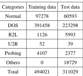
[image:18.595.226.370.613.745.2]

training and test datasets are listed in Table 1.

Table 1. The KDD CUP 1999 data set

Categories Training data Test data Normal 97278 60593

DOS 391458 223298 R2L 1126 5993

U2R 52 39

Probing 4107 2377 Others 0 18729

Total 494021 311029

algorithms: one with decision stumps and the traditional online Adaboost process, and the other with online

GMMs and our proposed online Adaboost process. Then, the performance of our PSO and SVM-based

distributed intrusion detection algorithm is evaluated.

5.1. Local models

For the online local models, the ability to handle mixed features, the effects of parameters on detection

performance, and the ability to learn new types of attacks are estimated in succession. Finally, the performances

of our algorithms are compared with the published performances of the existing algorithms.

1) Handling mixed features

Table 2 shows, respectively, the results of the classifier with decision stumps and the traditional online

Adaboost and the classifier with online GMMs and our online Adaboost, when only continuous features or both

continuous features and categorical features are used respectively, tested on the KDD training and test data sets

respectively. It is seen that the results obtained by using both continuous and categorical features are much more

accurate than the results obtained by only using continuous features. This shows the ability of our algorithms to

[image:19.595.94.498.356.435.2]

handle mixed features in network connection data.

Table 2. The results obtained by using only continuous features or both continuous and categorical features

Algorithms Features Detection Training data Test data rate

False alarm rate

Detection rate

False alarm rate Decision stump +

Traditional online Adaboost

Only Continuous 98.68% 8.35% 90.05% 13.76% Continuous + Categorical 98.93% 2.37% 91.27% 8.38% Online GMM + Our online

Adaboost

Only Continuous 98.79% 7.83% 91.33% 11.34% Continuous + Categorical 99.02% 2.22% 92.66% 2.67%

2) Effects of parameters on detection performance

In the following, we illustrate the effects of important parameters, i.e. the adaptable initial weight parameter

r in (32), the data distribution weight coefficient “1/M” in (4), the parameter



in (23), the parameter



in

[image:19.595.156.440.562.645.2]

(29), and the attenuation coefficient parameter



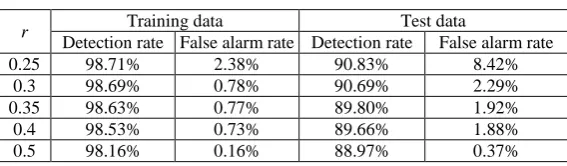
in (25).

Table 3. The results of the algorithm with decision stumps and the traditional online Adaboost when adaptable initial weights are used

r Training data Test data

Detection rate False alarm rate Detection rate False alarm rate 0.25 98.71% 2.38% 90.83% 8.42%

0.3 98.69% 0.78% 90.69% 2.29% 0.35 98.63% 0.77% 89.80% 1.92% 0.4 98.53% 0.73% 89.66% 1.88% 0.5 98.16% 0.16% 88.97% 0.37%

Table 3 shows the results of the algorithm with decision stumps and the traditional online Adaboost when

the adaptable initial weights formulated by (32) are used. When r is increased the detection rate and the false alarm rate are decreased. An appropriate setting of r is 0.3, as with this value of r, the false alarm rate of 2.28% is much smaller than the false alarm rate of 8.42% obtained by choosing r as 0.25, while an acceptable detection rate of 90.69% is still obtained. As shown in Table 2, when an identical initial weight is used for each training

rate of 91.27% is obtained on the test data, but the false alarm rate is 8.38%, which is too high for intrusion

detection. After adaptable initial weights are introduced, although the detection rate is slightly decreased, the

false alarm rate is much decreased, producing more suitable results for intrusion detection. This illustrates that

adjustable initial weights can be used effectively to balance the detection rate and the false alarm rate.

Table 4 shows the results of the algorithm with online GMMs and our online Adaboost when the data

distribution weight “1/M” in (4) and adaptable initial weights are used or not used. It is seen that when the

[image:20.595.112.482.264.373.2]

parameter M is not used, the false alarm rate is 54.15%, which is too high for intrusion detection. When the parameter M is used, the false alarm rate falls to 4.82%. When adaptable initial weights are used (r is set to 0.35) the false alarm rate further falls to 1.02%, while an acceptable detection rate is maintained.

Table 4. The results of our online Adaboost algorithm based on online GMMs with or without adaptable initial weights and the data distribution weight “1/M”

Parameters

Training data Test data

Detection rate False alarm rate Detection rate False alarm rate

Without the data distribution

weight “1/M” 99.86% 48.85% 97.49% 54.15%

With “1/M” and without

adaptable initial weights 99.22% 8.10% 91.74% 4.82% With “1/M” and adaptable

initial weights 98.91% 2.65% 90.65% 1.02%

Parameters



in (23) and



in (29) influence the detection results. Table 5 shows the detection rates

and false-alarm rates of the algorithm with online GMMs and our online Adaboost when





0

or 0.1 and

1





or 0.8. From this table, the following two points are deduced:

 When



is set to 0, the false alarm rate is very high. This is because the weak classifiers are chosen

only according to the false classification rate



_t, without taking into account the current sample.

Adopting the measure



_t of the combined classification rate balances the effects of “historical”

samples and the current sample, and then results in more accurate results.

 When



is set to 1, the detection rate is too low. This is because under this case only



_t is used to

weight the weak classifiers, i.e. every weak classifier is weighted in the same way as in the offline

Adaboost and the traditional online Adaboost. In the online training process, weighting every weak

classifier only using



_t causes over-fitting to some weak classifiers. Namely, the ensemble weights of

weak classifiers based only on



_t are not accurate. Weighting weak classifiers by combining



_t and

[image:20.595.198.397.698.765.2]

“contributory factors” yields the better performance.

Table 5. The results of the algorithm with online GMMs and our online Adaboost when 0or 0.1 and 0.8 or 1

Detection rate False alarm rate

0

   0.8 96.22% 77.66%

0.1

 ,  1 85.36% 0.60%

0.1