Munich Personal RePEc Archive
Information Cycles and Depression in a
Stochastic Money-in-Utility Model
Horii, Ryo and Ono, Yoshiyasu
Tohoku University, Osaka University
18 February 2009
Information Cycles and Depression
in a Stochastic Money-in-Utility Model
∗
Ryo Horii
†and Yoshiyasu Ono
‡Version: February 18, 2009
Abstract
This paper presents a simple model in which the learning behavior of agents generates fluctuations in money demand and possibly causes a prolonged de-pression. We consider a stochastic Money-in-Utility model, where agents re-ceive utility from holding money only when a liquidity shock (e.g., a bank run) occurs. Households update the subjective probability of the shock based on the observation and change their money demand accordingly. In this setting, we first derive a stationary cycles under perfect price adjustment, which is characterized by periods of gradual inflation and sudden sporadic falls of the price level. When the nominal stickiness is introduced, the liquidity shock is followed by a period of low output. We show that the adverse effects of the shocks are largest when they occur in succession in an economy which has enjoyed a long period of stability.
JEL Classifications: E32, E41, D83
Keywords: Bayesian Learning, Money Demand, Hamilton-Jacobi-Bellman Equations, Markov Modulated Poisson Processes, Partial Delay Differential Equations
∗The authors are grateful to Jun-ichi Itaya, Yasutomo Murasawa, and seminar participants at
Hitotsubashi University, Osaka Prefecture University, Okayama University and Vienna University for their helpful comments and suggestions. This research is partially supported by JSPS Grant-in-Aid for Young Scientists (B) 16730097, and is a part of the Osaka University 21st Century COE program, the Ministry of Education, Science, Sports and Culture.
†Correspondence: Graduate School of Economics, Tohoku University, 27-1 Kawauchi, Aoba-ku,
Sendai 980-8576, Japan; Tel/Fax: +81-(0)22-795-4272.
‡Institute of Social and Economic Research, Osaka University, 6-1 Mihogaoka, Ibaraki-shi,
1
Introduction
This paper presents a simple model in which the learning behavior of agents generates
fluctuations in money demand and possibly causes a prolonged depression. It is commonly assumed in monetary macroeconomics models–both in money-in-utility models and cash-in-advance models–that the benefit from holding money is well known beforehand. However, we sometimes find ourselves not very sure about how much money will be needed but hold some just for precaution. For concreteness, suppose that we can do business using checks at normal times, but once some shock to the financial system (e.g., a bank run) occurs transactions cannot be settled without money. We do not know exactly when bank runs occur. Moreover, we do not know the precise probability that bank runs occur but have to learn from past history. In such a situation, the learning process will cause the money demand to fluctuate, which in turn affect other macroeconomic variables especially when prices are not fully flexible.
To examine this information-drivenfluctuation, we introduce a stochastic version of Sidrauski’s (1967) model: agents receive utility from holding money only when a liquidity shock occurs. In the model, the shock is generated by a Markov modulated Poisson process (MMPP), which means that shock follows a usual Poisson process, and the arrival rate changes unobservably between high (a dangerous state) and low (a safer state) according to a Markov Process. We show that if the shock does not occur for a while, agents gradually increase the belief of being in a safer state, reduce the shock probability, and lower money demand, causing inflation. Conversely, when they observe the shock, they strengthen the belief that they are in a dangerous state, increase their subjective probability for meeting with the shock again, and raise money demand, causing deflation.
2000s. As agents become quickly pessimistic, the aggregate money demand jumps up, which can a cause depression if the prices are not fully flexible. Moreover, as in the case of Japan, the recovery from the depression is shown to take a long time when the agents’ pessimistic belief is so strong that it is not easily turned over by the gradually revealed information that no shock occurs.
There exist a number of earlier studies that analyzed the macroeconomic move-ments when an underlying state is only partially observable and information is re-vealed gradually (e.g., Caplin and Leahy 1993; Zeira 1994; Boldrin and Levine 2001; and Andolfatto and Gomme 2003). In particular, Chalkley and Lee (1998) con-sidered unobservable changes in investment opportunities and showed that recovery from a recession is protracted when risk aversion of agents prevents them from acting promptly on receiving good news. Potter (2000) and Nieuwerburgh and Veldkamp (2006) explained slow recovery generated by an endogenous flow of information. If agents have a pessimistic belief, their activities are low, generating less public information, and therefore good news is only slowly revealed. These studies are complementary to this paper in providing alternative explanations of slow recovery,1
but they do not show that negative shocks have the largest effect when the shocks hit an economy that was previously in good condition for a long time. This paper is also related to Farzin, Huisman and Kort (1998), Hassett and Metcalf (1999), Venegas-Mart´ınes (2001), and W¨alde (1999, 2005) in that the analysis includes a continuous-time stochastic optimization with discrete jumps in a state variable, al-though these studies consider the case in which agents know the true arrival rate of jumps.2
The organization of the paper is as follows. After introducing a stochastic Money-in-Utility model in Section 2, we describe the process of the liquidity shock and the evolution of the belief that is updated based on Bayes’ law in section 3. Section 4 presents a benchmark result for the case where the price level is perfectly flexible,
1
In our model, the recovery is slow not because information is scarce in depression but people’s strong beliefs dwarf the significance of new, favorable information. In fact, the flow of information brought by no occurrence of the shock is largest when people are convinced of being in the dangerous state. However, it is also the time when their prior belief is strongest, and hence people only slowly change it.
2Technically speaking, the substantial differences are in that our model have multiple state
and shows the pattern of price movements. The nominal stickiness is introduced in Section 5 to investigate how a depression is triggered and how economy recovers from it. Section 6 concludes the paper. Some mathematical proofs are collated in Appendix.
2
A Stochastic Money-in-Utility Model
This section sets up a stochastic Money-in-Utility model, where money holdings af-fect utility only at random discrete points in time. In the model, time is continuous,3
and the economy is inhabited by a continuum of infinitely lived homogeneous house-holds with measure one. At each date, they gain utility u(ct) from consumption ct, where instantaneous felicity function u(·) is twice differentiable, u0(·) > 0, and
satisfies the Inada conditions. In addition, when a liquidity shock occurs, they expe-rience utility loss v(mt)< 0 according to their real money holding mt. We assume v0(m) >0, which means that the size of utility loss is small when their real money
holdings are large. Function v(·) also satisfies v00(m) <0, lim
m→0mv0(m) >0, and
limm→∞v0(m) = 0. Their expected utilityEUt is therefore given by
EUt=Et
⎡ ⎣Z ∞
t
u(cτ)e−ρ(τ−t)dτ +
X
τ∈S(t,∞)
v(mτ)e−ρ(τ−t)
⎤
⎦, (1)
where ρ is the subjective discount rate and S(t,∞) is the set of future dates at which
the shock occurs. Note that the shock dates S(t,∞) are stochastic and cannot be
exactly anticipated in advance. Therefore, households are willing to hold money at all times for precaution.
We keep the remaining settings as simple as possible. Each household is endowed with one unit of labor at each point time, which is suppled to the labor market inelastically. A representative firm employs nt units of labor and competitively
pro-duces ynt units of goods, where y > 0 is a constant technology parameter and nt
is labor input. Note that, as long as prices are perfectly flexible, nt = 1 holds and
the output will be y. The monetary authority issues a constant amount of nominal money stock, the size of which is normalized to one.4 Goods are perishable and thus
cannot be stored. The households will not borrow or lend among themselves because
3
We use a continuous time model in order to highlight the difference between the change in belief when bad news arrives and when there is no such news. This strategy is similar to Driffill and Miller (1993) and Zeira (1999), but in their models uncertainty eventually vanishes and the economy reaches a steady state since unobservable state is time invariant.
4
they are identical. The firm has no value because of its linear production technology and perfect competition. Therefore, money is the only asset in this economy.
Let pt denote the price of consumption good. Since firms are competitive, the
nominal wage rate is given by the nominal marginal product pty. Then, the nominal
money holding of the household evolves according to
˙
Mt =ptynt−ptct. (2)
The objective of the representative household is to maximize expected utility (1) under budget constraint (2). To solve this problem, they need two sorts of additional information. One is the likelihood of encountering a shock in the future, because it determines the expected benefit of holding money. The next section explains how household estimate and update the likelihood through Bayesian learning. The other required information is the inflation rate, because it determines the real cost of holding money. We later investigate how the evolution pattern of the inflation rate is determined in the market, both for the case of perfectly flexible prices (Section 4) and for the case of sticky prices (Section 5).
3
Learning Process
There are two underlying states with different probabilities of the shock, called states H and L. In state i∈{H, L}, the shock occurs with probability θi per unit of time,
where θH > θL > 0. The household cannot directly observe the current state but
knows that the state evolves according to a Markov process: state H changes to state L with Poisson probability pH per unit of time whereas state L changes to state H
with probabilitypL. We assume that the shock occurs much more frequently in state
H than in state L and that the state change is a rare event when compared to the shock in state H. Formally,
Assumption 1 θH −θL> pH +pL.
By observing whether the shock occurs or not the household continuously revises its subjective shock probability in a Bayesian manner. Let θt ∈{θH,θL} denote the
true shock probability at time t, which is unknown to the household. Using infor-mation available up to time t, it forms a belief that currentθt isθH with probability
λH
t and θL with probabilityλLt. Obviously, λLt +λ
H
t = 1 for all t. (3)
In order to find how the household updates λi
t from t to t +∆t,5 we first
ob-tain the subjective probability that the shock does not occur between t and t+∆t
for given λi
t. It is denoted by Probt £
S(t,t+∆t] =∅
¤
, where Probt[·] is a probability
operator based on information available at t, S(a,b] is the set of dates on which the
shock actually occurs during (a, b], and ∅ the empty set. Since the underlying state is either H or L at time t +∆t, this probability is divided into two components, Probt
£
S(t,t+∆t]=∅ ∩θt+∆t=θH ¤
and Probt £
S(t,t+∆t]=∅ ∩θt+∆t=θL ¤
.
Each of the two components is further divided into two probabilities. The former is the sum of the probability that ‘the state is H at timetand neither the state change nor the shock occurs during the interval’ and the probability that ‘the present state is L and the state changes to H during the interval.’ It is6
Probt £
S(t,t+∆t] =∅ ∩θt+∆t =θH ¤
=¡1−(θH +pH)∆t¢λHt + (p L
∆t)λLt. (4)
Similarly, the latter is Probt
£
S(t,t+∆t]=∅ ∩θt+∆t =θL ¤
=¡1−(θL+pL)∆t¢λLt + (p H
∆t)λHt . (5)
Summing up (4) and (5) yields Probt
£
S(t,t+∆t]=∅
¤
= 1−θe
t∆t, (6)
where θe
t represents the expected (or subjective) probability of the shock per unit of
time at time t,
θe t ≡θ
HλH t +θ
LλL
t. (7)
Let us consider how the representative household updates its belief if it eventually
finds that the shock did not occur during (t, t+∆t]. In this case the information that S(t,t+∆t]=∅is added to its knowledge. Thus, using Bayes’ law wefind updated
subjective probability λi
t+∆t to be λi
t+∆t ≡Probt+∆t £
θt+∆t=θi ¤
= Probt £
θt+∆t=θi|S(t,t+∆t]=∅
¤
= Probt
£
S(t,t+∆t]=∅ ∩θt+∆t=θi ¤
Probt £
S(t,t+∆t]=∅
¤ .
5
Time interval ∆t is taken to be so short that the probability that the liquidity shock and a state change coexist in the interval is negligible.
6
Since the numerator is given by (4) or (5) and the denominator by (6), λH
t+∆t equals7 λHt+∆t =
¡
1−(θH +pH)∆t¢λH
t + (pL∆t)λLt
1−θe t∆t
.
From this equation we derive the time derivative of λH t as
˙
λHt = lim
∆t→0
λH
t+∆t−λHt
∆t = (θ e t −θ
H
−pH)λHt +p L
λLt. (8)
We next consider the case where the shock occurs during (t, t+∆t]. Since Probt
£
S(t,t+∆t]=6 ∅ ∩θt+∆t=θi ¤
=θiλit∆t for i∈{L, H}, (9)
the probability that the shock occurs is Probt
£
S(t,t+∆t]6=∅
¤
=¡θHλHt +θ L
λLt ¢
∆t =θte∆t, (10)
which is consistent with (6). From Bayes’ law dividing (9) by (10) gives the updated subjective probability that θt+∆t = θi under the condition that the shock occurs
during (t, t+∆t]. It is
λit= lim t0→t−
θiλi t0
θe t0
≡ θ iλi
t−
θe t−
, (11)
where subscript t−represents the state just beforet.8 Finally, we obtain the
dynam-ics of subjective probability θe
t. From (3) and (7), λH
t =
θe t −θL θH −θL, λ
L t =
θH −θe t
θH −θL. (12)
Substituting (8) and (12) into the time derivative of (7) yields the time derivative of
θe
t in the case where the shock does not occur at timet,
˙
θte = (θ e t −θ
L
−pL)(θte−θ H
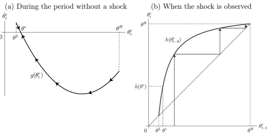
−pH)−pLpH ≡g(θet) for t /∈S(0,∞). (13)
Under Assumption 1, function g(θe
t) has a U-shape, as illustrated in Figure 1(a).
This function satisfies
g(θ)Q0⇐⇒θRθ∗ for any θ ∈£θL,θH¤, where
θ∗ ≡ θ
L+θH +pL+pH −p(θH +pH −θL−pL)2+ 4pLpH
2 ∈(θ
L
,θH). (14)
7λL
t+∆t is analogously obtained. From (3) it equals 1−λHt+∆t.
8Mathematically, θ
t− is the limit ofθτ as τ approachest from the left. θt− is different from θt
(a) During the period without a shock (b) When the shock is observed
Figure 1: Movement of belief through Bayesian learning
Similarly, by substituting (11) and (12) into (7) we obtain the value of θe t as a
function of θe
t− in the case where a shock does occur at time t.
θe t =θ
L+θH − θ
LθH
θe t− ≡
h(θe
t−) for t∈S(0,∞). (15)
As shown in Figure 1(b), function h(θ) satisfies
h(θH) =θH, and θe < h(θe)<θH for all θe∈(θL,θH).
Equations (15) and (13) respectively describe the dynamics ofθe
t with and without
the shock. They jointly show thatθe
t fluctuates within interval ¡
θ∗,θH¤. The liquidity
shock is a rare event, and therefore causes a discrete change in people’s expectation about the present state once it occurs. As function h(θe) is located above the
45-degree line in Figure 2, the more often people observe the shock, the more strongly they believe that they are in state H, and hence θe
t becomes closer to θH.
Conversely, in the absence of the shock people gradually become more and more optimistic and confident that the economy is in state L. Thus, their subjective prob-ability of the shock gradually declines, converging to θ∗.9 However, the U-shape of
function g(θe
t) implies that the speed of adjusting belief is slow when θet is near θH.
Note thatθe
t ≈θH is equivalent toλHt ≈1 from (12), which means that the precision
9θe
t never becomes lower thanθ∗(>θL) since people take into account the possibility that state
of the prior belief is quite high (i.e., people are quite sure that the current state is H). In that case any additional information has only a small impact on the posterior belief.
4
Information Cycles under Perfectly Flexible Prices
Let us examine how the market price evolves when households update their belief in the way explained in the previous section. In this section, we assume that price level ptcan be adjusted instantly so that nt = 1 holds for allt. Note that there is no
steady state in equilibrium at which the price level stays constant for all t because the decisions of household depend on θe
t, which is not constant. Thus, we instead
search for a stationary relationship between θe
t and pt. Specifically, we search for a
function p(·) that satisfies10
pt=p(θet) for allt. (16)
Since we are interested in a monetary equilibrium path in which money has a positive value, we limit our attention to the path of equilibrium price that become neither zero or infinity:11
Assumption 2 p(θe)∈(0,∞) for all θe ∈(θ∗,θH).
If the price level is a function of θe
t holds, the inflation rate can also be written as a
function of θe
t. From (16) and (13), πt≡p˙t/pt =
p0(θe t) p(θe
t)
g(θte)≡π(θ e
t) for t /∈S(0,∞). (17)
However, recall that the belief θe
t jumps when a shock is observed. In that case, pt
may also jump. The following gives the ratio of the price level between before and after the shock.
Πt≡pt/pt−=
p(h(θe t)) p(θe
t)
≡Π(θte) for t ∈S(0,∞). (18)
10
This approach is similar to Lucas (1978).
11To see why this assumption is reasonable, suppose thatp
t0 =∞for some datet0, which means that money has no value at t0. Then, it follows that pt = ∞ for all t ≥ t0 since otherwise an
arbitrage opportunity arises: consumers can obtain an arbitrary amount of money at date t0 at
no cost and then sell money (i.e., purchase goods) at a date in which pt is finite to increase their
expected utility. Since θe
t evolves within (θ∗,θH) recurrently, (16) implies that if p(θ∞) =∞ for
some θ∞∈(θ∗,θH) thenp(θe) =
∞for allθe
∈(θ∗,θH). That is, if there is suchθ∞, thenp t=∞
for alltand therefore money is never demanded. We also rule out the possibility thatp(θe) = 0 for
some θe
Our task is tofind a functionp(θe
t) (and therefore alsoπ(θet) andΠ(θte)) such that,
given these, the household’s optimization leads to the clearance of all markets. In the following, we will proceed in three steps: (i) We consider a dynamic programming problem and obtain a Hamilton-Jacobi-Bellman (HJB) equation, given π(θe
t) and
Π(θe
t). (ii) We obtain the Euler equation from thefirst order and envelope conditions
of the HJB equation. (iii) We substitute the equilibrium conditions to the Euler equation and examine the properties that must be satisfied by function p(θe
t).
When the inflation rate follows (17)-(18) andnt= 1 holds, budget constraint (2)
can be written as
˙
mt=y−π(θet)mt−ct for t /∈S(0,∞), (19)
mt=mt−/Π(θte) for t∈S(0,∞). (20)
The household maximizes the expected utility (1) subject to (19) and (20), and also to the law of motion of thier belief (13) and (15). LetU(θe, m) denote the maximized
value when the current belief and real money holding are θe and m. By considering
a small time interval ∆t, the Bellman equation for this problem can be written as
U(θe, m) = max c
h
u(c)∆t+ (θe∆t)v(m00)
+ 1 1 +ρ∆t
©
(1−θe∆t)U(θe0, m0) + (θe∆t)U(h(θ), m00)ªi, (21)
whereθe0 =θe+g(θe)∆t,m0 =m+ (y−π(θe)m−c)∆t, andm00=m/Π(θe). Observe
that with probability 1−θe∆t there is no shock and the state changes from (θe, m)
to (θe0, m0), whereas with probability θe∆t there is a shock and the state changes to
(h(θe), m00). Taking the limit ∆t → 0 in (21) yields the Hamilton-Jacobi-Bellman
(HJB) equation for the problem:
ρU(θe, m) = max
c h
u(c) +θe¡v(m/Π(θe)) +U(h(θe), m/Π(θe))−U(θe, m)¢ +g(θe)U
θ(θe, m) +
¡
y−π(θe)m
−c¢Um(θe, m) i
.
(22)
Differentiating the right hand side of (22) with respect to c gives the first order condition
u0(ec) = U
m(θe, m), (23)
where ec denotes the optimal amount of consumption. Since θe
t and mt evolves
ac-cording to (13) and (19) during the period of no shock, equation (23) shows that the movement of consumption is characterized by
d dtu
0(ec
t) =g(θte)Umθ+
¡
abbreviating the arguments for U(·,·) functions when they are (θe, m). From the
envelope theorem, (22) can be differentiated with respect to m at c=ecto give (ρ+π(θe) +θe)Um =g(θe)Uθm+
¡
y−π(θe)m−ec¢Umm
+θeΠ(θe)−1¡v0(m/Π(θe) +U
m(h(θe), m/Π(θe)) ¢
. (25)
By substituting (23) and (24) for (25), we can eliminate the value function from it to obtain the Euler equation,
d dtu
0(ec
t) = (ρ+π(θe) +θe)u0(ect)−θe v0(m
t/Π(θe)) +u0(ec00t)
Π(θe) for t /∈S(0,∞), (26)
where ec00
t represents the optimal amount of consumption when a shock is observed
and the state changes to (h(θe
t), m/Π(θte)).
Since all households are symmetric, the equilibrium of goods and money markets implies
ect(=ec00t) = y, mt=p(θet)−1 for all t. (27)
Function p(·) is determined so that the household’s demand for goods and money always satisfies (27). Substituting (27) into (26) yields a condition that must be satisfied for all possible values of θe,
ρ+π(θe) =θeΠ(θe)−1v0(p(h(θe
))−1) +θe¡Π(θe)−1−1¢. (28) The left hand side represents the cost of holding money: the utility loss from post-poning consumption plus the capital loss caused by inflation. In the other side are the expected benefits of holding money: the first term is the expected utility from holding money, whereas the second term represents the expected capital gain by the downward jump in the price level (the upward jump in the value of money) when the liquidity shock occurs. Thus, (28) shows that function p(·) is determined so that the cost and the benefit of holding money are equalized with each other.
From (17), (18) and (28), we obtain a (delay) differential equation for p(·):
p0(θe) = p(θ e) g(θe)π(θ
e), where
π(θe)
≡ −(ρ+θe) +θe p(θ e) p(h(θe))
v0(p(h(θe))−1) +u0(y)
u0(y) .
(29)
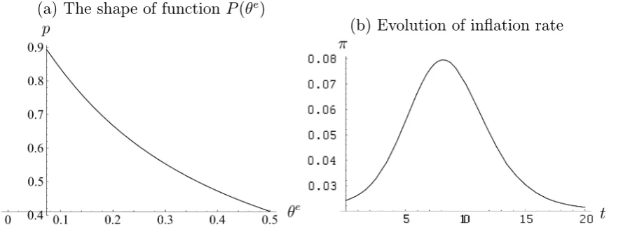
(a) The shape of function P(θe)
[image:13.595.88.533.99.268.2](b) Evolution of inflation rate
Figure 2: Inflation cycles without nominal frictions
Lemma 1 Under Assumption 2 and transversality condition12
lim
T→∞Ete
−ρ(T−t)u0(c
T)mT = 0 for all t, (30)
function π(·) must satisfy limθe→θ∗π(θe) = 0.
proof: in appendix
Intuitively, the inflation rate at the limit (θe
t → θ∗) must be must be equalized to
the growth rate of nominal money supply, which is zero in our model. Note that there exists a non-zero possibility that the liquidity shock does not occur for an arbitrary long time. In that case, if limθe→θ∗π(θe) 6= 0, the real money holding
mt=p−t1 diverges to either infinity (violating the transversality condition) or to zero
(violating the assumption of the monetary equilibrium).
The stationary dynamics of a monetary equilibrium can be calculated from (29) and the boundary condition given by Lemma 1. Figure 2(a) shows the representative shape of function p(·) against θe, which is downward sloping.13 A large value of θe t
means that people anticipates that the liquidity shock occurs with a high probability. In that situation, the marginal benefit of holding money is high. Thus, to clear the market for money, the value of money must be sufficiently high in relative to the value of good, which means a low price level.
During the period without the liquidity shock, θe
t gradually declines and pt
in-creases. Figure 2(b) shows the evolution of inflation rate against time as θe
t moves
12Operator E
t represents the expectation based on the information available to agents at datet.
13In all examples presented in this paper, we specifyu(c) = lnc, v(m) =
−m−1,y= 1,ρ=.05,
θH= 1,θL=.2,pH=.05 andpL=.02. We have con
from θH to θ∗. Inflation accelerates temporarily when the households adjusts their
belief responding to observing no shock for a certain time length, but it gradually falls to the rate of nominal money growth, which is zero in this case, as the economy converges to the most optimistic state. When the liquidity shock occurs, θe
t jumps
up. Then pt jumps down so that the (θet, pt) pair is always on the curve depicted in
panel (a). Thus, the dynamics of the economy is characterized by gradual inflation with sporadic and discrete falls in the price level.
At each event of the liquidity shock, price level must jump down in order to clear the increased liquidity demand induced by the change in people’s belief. However, we rarely observe such a discrete fall in the price level in the aggregate economy; although we do sometimes observe a discrete fall in the prices of certain goods, the aggregated general price level tends to fall only slowly. One explanation for this is the existence of a (downward) nominal stickiness in the price level caused by staggered price adjustments, menu costs, labor unions, moral issues, and the all other factors discussed in the literature. If the price cannot jump downward, our model predicts that the demand for money exceeds the supply, and, by Warlas’ law, a demand shortage occurs in the goods and labor market. The next section investigates this possibility.
5
Possibility of Depression under Sticky Prices
The discrete fall in the price level derived in the previous section implies that the instantaneous rate of inflation must be minus infinity. This section considers a more realistic setting where the price level cannot fall infinitely fast, or equivalently, where the rate of deflation is restricted to be within somefinite bound.14 Let us consider a
model similar to the one analyzed in the previous section, with a only difference in
14This is equivalent to assuming that the nominal wage cannot fall in
that the price level cannot fall faster than a certain rate,15
˙
pt/pt≥ −δ, δ∈(0,∞). (31)
Note that condition (31) breaks the one-for-one relationship between the price level and the belief because pt cannot jump whileθet can. Thus, the state of the economy
cannot be described solely by θe
t; but by the pair of (θet, pt). This economy has two
possibilities at each point in time. The first possibility is that constraint (31) is not binding and full employment obtains (nt = 1 and ct = y). The second possibility
is that (31) is binding, i.e., p˙t/pt = −δ, and unemployment exists (nt < 1 and ct< y). Which one of these possibilities occurs depends on the state of the economy,
summarized by (θe t, pt).
It is natural to guess that, for a given level of θe
t, there is a level of pt at which
the money market clears and full employment obtains. Let us denote this critical level by p(θe
t). Price level pt cannot be below the threshold p(θe) since there is no
upward stickiness in the price level and thus can be adjusted instantly if pt < p(θe).
Similarly to the previous section, we limit our attention to the monetary equilibrium path by assuming that16
Assumption 3 p(θe)∈(0,∞) for all θe ∈(θ∗,θH).
Unemployment occurs when constraint (31) is binding, i.e., when p > p(θe). In
this case, the economy experience deflation at the rate of δ. If (31) is not binding, full employment obtains and the price level evolves so that equilibrium condition
p =p(θe) is maintained. Let us denote by C(θe, p) aggregate demand for goods at
state (θe, p). Then,
C(θe, p) (
=y if p=p(θe),
< y if p > p(θe). (32)
15
To keep the analysis to follow as tractable as possible, we employ a quite simple specification for the sticky price in condition (31). This assumption is motivated by the experience in Japan, where the rate of deflation remained at a few percentage points for nearly ten years after mid 1990s. When we explicitly model a staggered pricing behavior by monopolistically competing firms, the rate of deflation would differ depending on the state of economy. Nonetheless, the most of the main implications will not change because the most crucial assumption is that the price cannot jump. We could also assume a symmetric restriction such asp˙t/pt∈[−δ,δ]. This would make the analysis
a little complicated without changing the final results.
16
We can show that if there is someθ∞∈(θ∗,θH) such thatp(θ∞) =∞thenp
The inflation rate for a given state can be summarized as
π(θe, p) =
⎧ ⎪ ⎨ ⎪ ⎩
p0(θe) p(θe)g(θ
e
) ifp=p(θe), −δ if p > p(θe).
(33)
The representative household maximize (1) under budget constraint (2). Since the demand for goods is C(θe
t, pt) and the production function is ynt, the amount
of employment is determied as nt=C(θet, pt)/y. The budget constraint can thus be
written as
˙
mt=C(θet, pt)−π(θte, pt)mt+ct (34)
as long as pt evolves continuously, and as (20) if pt jumps. Note that, from (31),
price level pt never jumps down. At this point, however, we cannot rule out an
upward jump in pt, which may occur if current price level pt is smaller than the
new market clearing price level after the shock, p(h(θe
t)). Let us denote the value
function of the household by U(θe, p, m), which now depends on the current value
of pbecause it affects the aggregate demand and thus the household’s income. The Bellman equation for this problem is
U(θe, p, m) = max c
h
u(c)∆t+ (θe∆t)v(m00)
+ 1 1 +ρ∆t
©
(1−θe∆t)U(θe0, p0, m0) + (θe∆t)U(h(θe), p00, m00)ªi, (35)
whereθe0 =θe+g(θe)∆t,p0 =p+π(θe, p)p∆t,m0 =m+ (C(θe, p)
−π(θe, p)m+c)∆t, p00 = max{p(h(θ)), p}, andm00 = (p/p00)m. Taking the limit of∆t→0 in (35) yields
the HJB equation,
ρU = max
c h
u(c) +θe¡v(m00) +U(h(θe
), p00, m00)−U¢+g(θe
)Uθ
+π(θe, p)pUp+ ¡
C(θe, p)−π(θe, p)m−c¢Um i
,
(36)
where the arguments of function U(·,·,·) and its partial derivatives are abbreviated when they are (θe, p, m). The first order condition for (36) is u0(ec) = U
m(θe, p, m),
where ec is the optimal amount of consumption. Then, the envelope condition is (ρ+π(θe, p) +θe)U
m =θe(p/p00) ¡
v0(m00) +U
m(h(θe), p00, m00) ¢
+g(θe)U
θm
+π(θe, p)pUpm+ ¡
C(θ, p)−π(θe, p)m−ec¢Umm.
(37)
p(h(θe)) and therefore p00 = p and m00 = m. The following analysis focuses on this
case and we leave for Appendix the analysis of the case of p < p(h(θe)).
Substituting the first order condition, its time derivative, and the conditions for the representative household, ec = C(θe, p) and m = p−1, into (37) yields the Euler
equation,
à ρ−
d
dtu0(C(θ e, p)) u0(C(θe, p))
!
+π(θe, p) =θe v0(p−1) u0(C(θe, p)) +θ
e µ
u0(C(h(θe), p)) u0(C(θe, p)) −1
¶
(38)
for all t /∈ S(0,∞). Equation (38) has an interpretation similar to (28). The cost of
holding money, given by the LHS, is the sum of time preference and inflation. The benefit is the sum of the direct utility gain and the expected capital gain measured in terms of utility when a shock occurs and consumption jumps down.
Functionsp(·) andC(·,·) are determined so that equation (38) holds for all pos-sible pairs of (θe, p). Let us first consider the case in which current price p is at
the market clearing level p(θe). Recall that p = p(θe) implies C(θe, p) = y and π(θe, p) = p0(θe)g(θe)/p(θe) from (32) and (33). Substituting these for (38) gives a
differential equation that determines the form of function p(·):17
p0(θe
) = p(θ
e) g(θ)γp(θ
e
), where
γp(θe) =
−(ρ+θe) +θev0(p(θ
e)−1) +u0(C(h(θe), p(θe)))
u0(y) .
(39)
Function γp(θe) in (39) represents the growth (in
flation) rate of the market clearing price, p˙t/pt. The difference between (29) and (39) lies in the fact that consumption
is adjusted in the occurrence of the liquidity shock when nominal stickiness exists, while adjustment is done fully by the price level when price is completely flexible. A boundary condition for equation (39) is given by the following lemma.
Lemma 2 Under Assumption 3 and transversality condition (30), function γp(·)
must satisfy limθe→θ∗γp(θe) = 0
proof: in appendix
Next, consider the case in which current pricepis above the market clearing level
p(θe). In this case, p > p(θe) implies C(θe, p)< y and π(θe, p) = −δ. Substituting
17Equation (39) holds when p
≥ p(h(θe)). The corresponding expression for γ
p(θe) when p <
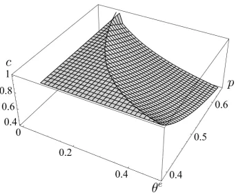
Figure 3: Representative shapes of function C(θe, p) and functionp(θe)
this for (38) gives a partial (delay) differential equation for function C(·,·),
g(θe)Cθ(θe, p)−pδCp(θe, p) =
u0(C(θe, p)) u00(C(θe, p))γu0(θ
e
, p), where
γu0(θe, p) =ρ−δ+θe−θe
v0(p−1) +u0(C(h(θe), p)) u0(C(θe, p)) .
(40)
In (40), γu0(θe, p) represents the rate of change in marginal utility, u˙0/u0. Combined
with the boundary conditionC(θe, p(θe)) =yfor allθe, this partial (delay) differential
equation determines the shape of function C(·,·) for all (θe, p)∈{(θe, p)|p > p(θe))}.
5.1
Numerical Analysis
Since p(·) and C(·,·) are interrelated as described above, they are determined si-multaneously so that they satisfy the system of partial differential equations, (39) and (40), along with two boundary conditions specified above. This problem can be solved numerically by combining a finite difference method and an appropraite iteration method.18 Figure 3 shows a representative shape of function C(·,·) in
18
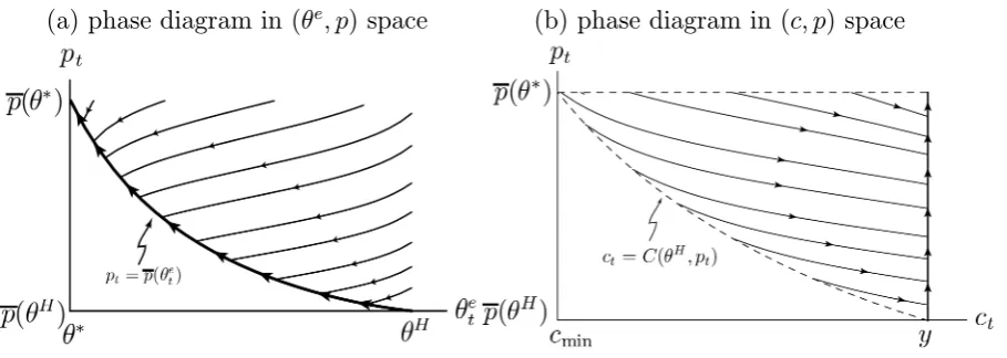
(a) phase diagram in (θe, p) space (b) phase diagram in (c, p) space
Figure 4: Evolution of the economy during the period of no shock.
(θe, p) space, where the solid curve on the edge represents function p(·). Observe
that function p(·) is downward sloping in θe. The reason behind it is the same as
the reason for the similar property of p(·) in the previous section: when θe is large,
people’s liquidity preference is high and thus a low price level (a high relative price of money to goods) is required to equalize the money demand to the money supply. The height of curved surface indicates the value of function C(θe, p) at each state in
region p > p(θe). C(θe, p) is equal to y on the curve of p = p(θe) and gets smaller
as the pair (θe, p) moves to the direction of north-east. That is, a pair of high θe t
and high pt implies a combination of high liquidity preference, a low relative price
of money to goods, and a small supply of real money stock. In that case, the excess demand for money is huge and therefore the aggregate demand for goods (and thus employment) is small.
Figure 4 illustrates the movement of the belief, price and consumption (output) during the period of no shock. For ease of visibility, we present two phase diagrams in (θe, p) spece and in (c, p) space. If the current price level p
t is higher than the
market clearing price level p(θe
t), the price gradually falls and consumption (output)
grows according to
˙
pt pt
=−δ, c˙t= u0(c
t) u00(ct)
"
ρ−δ+θe −θe
t
v0¡p−1
t ¢
+u0(c00
t) u0(ct)
#
, (41)
where c00
t ≡C(h(θe), pt).19 As long as no shock occurs, the pair (θe, pt) follows (41)
until it reaches the market clearing curve pt =p(θet) in a finite time. From that time
19The second equation in (41) is obtained by solving d dtu
0(c
t)/u0(ct) =γu0(θe, p), whereγu0(θe, p)
on, consumption stays constant and the price level rises so that the pair traces the market clearing curve,
˙
pt pt
=−(ρ+θe t) +θte
v0(p−1
t ) +u0(c00t)
u0(y) , ct=y. (42)
As θe approaches θ∗, the price level converges to p∗ ≡ p(θ∗), and inflation rate
converges to zero.
Now let us explain how the economy reacts to the liquidity shocks. In this model, the reaction is both qualitatively and quantitatively different depending on the history and the way the economy is hit by the shocks. To illustrate this point, the following consider three different examples. Figure 5(a) presents the result from a standard impulse-response exercise. In this exercise, it is assumed that there have been no shock for a long time and then the economy is hit by a one-shot liquidity shock. Before the shock, the household has the lowest possible belief θe = θ∗ and
the price level is at the highest, pt = p(θ∗). At the time of the liquidity shock, the
household updates its belief θe to h(θ∗), but p
t cannot jump immediately. Thus, as
illustrated in the left panel, the pair (θe, p
t) jumps horizontally toward east. This
means that the pair is now above the market clearing line (pt=p(θet)), and therefore
consumption and output must fall discretely (see the right panel). After the shock, both θe and p
t gradually falls through learning and deflation. This means that the
pair (θe, p
t) approaches the market clearing curve, and accordingly consumption and
output recover toward the initial level.
As a second example, Figure 5(b) illustrates a situation where the economy is hit regularly by shocks. Observe that, when compared to the case where the shock occurs only once, consumption falls only slightly each time the economy is hit by a shock, and that the recovery after the fall is fairly quick. There are two reasons behind this counter-intuitive result. When shocks occur regularly, the belief of the household is always near the highest level,θH. That is, the household believes almost
surely that the economy is in the dangerous state (state H), and will not change its belief much when another shock is observed. In addition, the price level is already adjusted to this belief and near the lowest level p(θH). Thus, even when θe
t jumps,
the price need not fall significantly. As a result, the recovery process is quick. Figure 5(c) displays the worst possibility as the third example. Similarly to example (a), we assume that there have been no shock for a long time before the economy is hit by a shock (this implies that the economy is initially at θe =θ∗ and
pt = p(θ∗)). However, in this example, the shock is not one-shot, but comes in a
bunch for a short while. By observing the shocks, the belief θe
(a)
(b)
[image:21.595.88.518.98.497.2](c)
Figure 5: Reaction of the economy to liquidity shocks: three examples
again nearly to the highest level θH, while giving little time for the price level to
adjust through deflation. As a result, the pair (θe, p
t) moves to the furthiest position
from the market clearling curve, and consumption (outout) falls nearly to the lowest possible value (cmin). In addition, even after the shock ceases, the recovery process is
slow; it can be seen from the figure that the time path ofct is convex in the phase of
recovery. This is because once the household hold a strong belief that the underlying state is bad (i.e., θe
t ≈θH), the belief cannot be easily overturned by the additional
information that no shock is observed for a while.20 In other words, once agents
become too pessimistic, it takes a long time until the recovery process accerelates.
20
(a) actual shock probability θt (dashed line) and belief θe t.
(b) actual price level pt (dashed curve) and market clearing price pt
[image:22.595.80.514.105.471.2](c) consumption ct
Figure 6: A simulated time path when shock are generated by Markov modulated Poisson process
This pattern of recovery is in contrast to example (a), where the shock is observed only once and may be viewed as a “mere accidient.” (Observe that the time path of
ct during the recovery process is actually concave in example (a)).
So far, we considered three examples where the shocks occur in specific patterns. However, in the actual model economy, the shocks are randomly generated by the Markov modulated Poisson process, as explained in Section 3. Figure 6 which depicts a simulated time path of the economy when shocks are randomly generated. Observe that the price level goes up when the economy stay in the safer fundamental state (state L) for some time. This is in fact dangerous because once the state switches to state H, where many shocks are likely to occur, the market clearing price (pt)
creates a large discrepancy between pt and pt, which translates into a period of
stagnation where consumptionct and thus output stay below the normal level. This
mechanism provides one possible reasion why once a long-time (seemingly) stable economy experiences negative shocks it has to go through a long and deflationary period of depression.
6
Conclusion
This paper presents a theory of economicfluctuations and prolonged depression based on households’ learning behavior. We consider a stochasic version of Money-in-Utility model, where agents recieve utility from money only when liquidity shocks occur, where the true shock probability unobservably changes between high and low. In this setting, we first exmained the way the households update thier belief through Bayesian learning. Second, using Hamilton-Jacobi-Bellman equations, we investigated the evolutions of consumption and money holding of the household who behaves rationally based on his belief about the state of the economy. Third, we derived a stationary cycle under perfect price adjustments in terms of a delay dif-ferential equation and demonstrated that the price level would experience sporadic downward jumps in such a setting. Forth, we extended the model to incorporate nominal stickiness. In this case, the belief and the slow-moving price cannot corre-spond one-to-one, and this discrepancy creates a period of stagnation. The stationary dynamics is given as a solution to a system of partial delay differential equations, which we solved numerically. It is shown that the reaction of the economy to negative shocks depends on the history and the pattern of the realization of the shocks. In particular, a successive occurrence of shocks may cause a depression if the economy has enjoyed a long period of stability before encountering the shocks.
Appendix
A
Analysis of the case of
p < p
(
h
(
θ
e))
Ifpt< p(h(θet)),p00 =p(h(θTe)) andm00=mp/p(h(θte)) in (35), (36) and (37).
e
c=C(θe, p) and m=p−1, into (37) yields the Euler equation,
à ρ−
d
dtu0(C(θ e, p)) u0(C(θe, p))
!
+π(θe, p)
=θe p p(h(θe))
v0(p(h(θe))−1)
u0(C(θe, p)) +θ e
µ p p(h(θe))
u0(y)
u0(C(θe, p))−1
¶ (43)
for allt /∈S(0,∞). Substitutingp=p(θe),C(θe, p) =yandπ(θe, p) =p0(θe)g(θe)/p(θe),
from (32) and (33), for (43) gives the growth rate of pt during the period of full
em-ployment:
γp(θe) =
−(ρ+θe) +θe p(θ e) p(h(θe))
v0(p(h(θe))−1) +u0(y)
u0(y) . (44)
When unemployment exists (i.e., p≥p(θe)), the rate of change in marginal utility is
obtained by substituting π(θe, p) = −δ for (43),
γu0(θe, p) =ρ−δ+θe+θe
p p(h(θe))
v0(p−1) +u0(y)
u0(C(θe, p)) . (45)
B
Proof of Lemmas
Let θns
t,T, cnst,T, pnst,T and mt,Tns denote respectively the values of θT, cT, pT and mT
conditional on that no shock occurs between t and T. Then, the probability that no shock occurs between t and T is given by exp³−RtT θ
ns t dτ
´
.
The transversality condition (TVC) can be written as limT→∞EtVt,T = 0, where Vt,T ≡e−ρ(T−t)u0(cT)mT and Et denotes the expectation taken upon the information
available at t. Since u0(c
T)mT ≥0 for all T, EtVt,T ≥exp
µ −
Z T
t
θtnsdτ ¶
e−ρ(T−t)u0(cns
t,T)mt,T ≡Vt,Tns. (46)
Note that while Vt,T is a random variable, Vt,Tns is a deterministic variable given the
information available at t. From (46), a necessary condition for the TVC is lim
T→∞V ns
t,T ≤0. (47)
Differentiating (46) with respect toT and using equilibrium conditionmns
t,T = 1/pnst,T
yield
dVns t,T/dT Vns
t,T
=−θns
t,T −ρ+
du0(cns t,T)/dT u0(cns
Lemma 1
Without nominal stickiness, cns
t,T =y for allT and thus du0(cnst,T)/dT = 0. From (29),
(dpns
t,T/dT)/pnst,T =π(θnsT ). Substituting these into (48) yields dVns
t,T dT =−θ
ns t,T
p(θns t,T) p(h(θns
t,T))
v0(p(h(θns
t,T))−1) +u0(y)
u0(y) V
ns
t,T. (49)
Using p(θns
t,T) =pnst,T = 1/mnst,T and the definition ofVt,Tnsin (46), equation (49) reduces
todVns
t,T/dT =−exp(− RT
tρ+θ ns
t,vdv)θnst,TZ(h(θt,Tns)), whereZ(θ)≡(v0(p(θ)−1) +u0(y))/p(θ).
Integrating this differential equation with respect to T from t to ∞ and using the fact that Vns
t,t =u0(y)mt give
lim
T→∞V
ns
t,T =u0(y)mt− Z ∞ t exp µ − Z T t
ρ+θnst,vdv ¶
θnst,TZ(h(θ ns
t,T))dT. (50)
Fix a small constant a >0 and define a closed interval A ≡ [h(θ∗), h(θ∗+a)]∈
(θ∗,θH). Note that Assumption 2 implies that Z(θ)
∈ (0,∞) for all θ ∈ (θ∗,θH).
In addition, it is continuous in this interval because (29) implies that p(·) is dif-ferentiable. Thus, there exist finite constants Zmin ≡ minθ∈AZ(θ) ∈ (0,1) and Zmax ≡ maxθ∈AZ(θ) ∈ (0,1). Whenever θte ∈ (θ∗,θ∗ +a), θnst,T ∈ (θ∗,θ∗+a) for all T ≥ t. and therefore there is upper and lower bounds for the second term in the RHS of (50), given by
µ θ∗Z
min
ρ+θ∗+a,
(θ∗+a)Z
max
ρ+θ∗
¶
≡(Imin, Imax)⊂(0,∞). (51)
Now suppose that limθe→θ∗π(θe) < 0. Then as θte converges to θ∗, pt → 0 and
therefore mt → ∞. However, this violates the TVC since conditions (47), (50) and
(51) imply that the TVC requires mt ≤Imax/u0(y) wheneverθet ∈(θ∗,θ∗+a).
Suppose conversely that limθe→θ∗π(θe)<0. Then asθet converges to θ∗, pt→ ∞
and thereforemt→0. For sufficiently smallmt, (50) and (51) imply limT→∞Vt,Tns <0.
SinceVns
t,t =u0(ct)mt>0 andVt,Tnsis continuous inT, there should be a value ofT ≥t
such that Vns
t,T = 0. From the definition of Vt,Tns in (46) this implies thatmnst,T = 0 and
therefore p(θns
t,T) =pnst,T =∞, violating Assumption 2.
Lemma 2
We first derive a contradiction under assumption limθe→θ∗γp(θe)<0. Fix a >0 and
define A = [h(θ∗), h(θ∗ +a)]. Then, from p(θ) ∈ (0,∞) and its continuity, there
exists pmin ≡minθ∈Ap(θ)∈(0,∞). The assumption limθe→θ∗γp(θe)<0 implies that p(θ) → 0 as θ → θ∗. Recall, in addition, that p
pt > p(θ∗). Thus, there is a positive probability that (θte,pt) pair satisfiesθet <θ∗+a
and pt ≤pmin when the liquidity shock does not occur for a sufficiently long while.
Suppose that the current (θe
t, pt) pair satisfies the above inequalities. Then pns
t,T < p(h(θnst,T)) for allT ≥t, which means that the analysis in Appendix A applies.
Substituting the results obtained in Appendix A into (48) yields
dVns t,T/dT Vns t,T = (
−θnst,T −ρ+γu0(θt,Tns) +δ if pnst,T > p(θt,Tns),
−θns
t,T −ρ−γp(θ ns
t,T) ifp ns
t,T =p(θ ns t,T).
(52)
Substituting (44) and (45) into (52) and using pns
t,T = 1/m ns
t,T and the definition of Vns
t,T in it, equation (52) reduces to dV ns
t,T/dT =−exp(− RT
tρ+θ ns
t,vdv)θt,TnsZ(h(θ ns t,T)),
where Z(θ) ≡ (v0(p(θ)−1) +u0(y))/p(θ). Integrating this differential equation with
respect to T fromt to ∞and using the fact that Vns
t,t =u0(cnst,T)mt give
lim
T→∞V
ns
t,T =u0(c ns t,T)mt−
Z ∞ t exp µ − Z T t
ρ+θns t,vdv
¶ θns
t,TZ(h(θ ns
t,T))dT. (53)
Note that h(θns
t,T) ∈ A for all T ≥ t and that there exists a finite constant Zmax ≡ maxθ∈AZ(θ). From cnst,T ≤ y, u0(cnst,T) ≥ u0(y) for all T. Thus (47) and (53)
jointly imply that
mt≤
(θ∗+a)Z
max
(ρ+θ∗)u0(y). (54)
While assumption limθe→θ∗γp(θe) < 0 implies that an arbitrarily large mt = 1/pt
realizes with a positive probability, the RHS of (54) is constant. Thus (54) and hence the TVC will be violated with a positive probability.
Next, assume conversely that limθe→θ∗γp(θe)>0, which means thatp(θe) become
arbitrarily large as θe → θ∗. Then, θns
t,T ∈ (θ∗,θ∗ +a) and pnst,T = p(θnst,T) > pmax ≡
maxθ∈Ap(θ) for sufficiently large T. In this case, Analysis in Section 4 applies and
full employment obtains. From mns
t,T = 1/pnst,T and (39), dmns
t,T
dT = (ρ+θ ns
t,T)mnst,T −θnst,T
v0(mns
t,T)mnst,T +u0(C(h(θnst,T),1/mnst,T))mnst,T
u0(y) (55)
for sufficiently large T. As T → ∞, p(θns
t,T) → ∞ and therefore mnst,T → 0. In
this case, (55) implies limT→∞dmnst,T/dT <θTnsu0(y)−1limm→0v0(m)m <0,where the
latter inequality follows from the definition of v(·). These properties jointly imply that there is a finiteT such thatmns
t,T = 0 and therefore p(θt,Tns) = pnst,T =∞, violating
References
[1] Andolfatto, David and Paul Gomme (2003), “Monetary Policy Regimes and Beliefs,”International Economic Review,44(1), 1-30.
[2] Boldrin, Michele and David K. Levine. (2001). “Growth Cycles and Market Crashes.” Journal of Economic Theory 96, 13—39.
[3] Caplin, Andrew and John Leahy. (1993). “Sectoral Shocks, Learning, and Ag-gregate Fluctuations.”Review of Economic Studies 60, 777—794.
[4] Chalkley, Martin and In Ho Lee (1997), “Learning and Asymmetric Business Cycles,”Review of Economic Dynamics, 1, 623-645.
[5] Driffill, John and Marcus Miller (1993), “Learning and Inflation Convergence in the ERM,”Economic Journal,103, 369-378.
[6] Dockner, Engelbert, Steffen Jørgensen, Ngo Van Long and Gerhard Sorger. (2000). Differential Games in Economics and Management Science.: Cam-bridge University Press.
[7] Farzin, Y. H.,Huisman, K. J. M., Kort, P. M. (1998) ”Optimal timing of tech-nology adoption,” Journal of Economic Dynamics and Control, vol. 22(5), pages 779-799.
[8] Hassett, Kevin A, Metcalf, Gilbert E (1999) ”Investment with Uncertain Tax Policy: Does Random Tax Policy Discourage Investment?,” Economic Journal, vol. 109(457), pages 372-93.
[9] Lucas, Robert E. Jr. (1978), “Asset Prices in an Exchange Economy,” Econo-metrica,46(6), 1429-1445.
[10] Nieuwerburgh, Stijn Van and Laura L. Veldkamp. (2006). “Learning Asymme-tries in Real Business Cycles.”Journal of Monetary Economics 53(4), 753—772. [11] Potter, Simon M. (2000), “A Nonlinear Model of Business Cycle,” Studies in
Nonlinear Dynamics and Econometrics, 4(2), 85-93.
[13] Venegas-Martinez, Francisco (2001) ”Temporary stabilization: A stochastic analysis,” Journal of Economic Dynamics and Control, vol. 25(9), pages 1429-1449.
[14] W¨alde, Klaus, (1999) ”Optimal Saving under Poisson Uncertainty,” Journal of Economic Theory, vol. 87(1), pages 194-217.
[15] W¨alde, Klaus (2005) ”Endogenous Growth Cycles,” International Economic Re-view, vol. 46(3), pages 867-894.
[16] Zeira, Joseph. (1994). “Informational Cycles.” Review of Economic Studies 61, 31—44.