http://dx.doi.org/10.4236/wjm.2016.64010
Numerical Simulation of Asymmetric
Merging Flow in a Rectangular Channel
Abuzar Abid SiddiquiDepartment of Basic Sciences, Bahauddin Zakariya University, Multan, Pakistan
Received 8 November 2015; accepted 19 April 2016; published 22 April 2016 Copyright © 2016 by author and Scientific Research Publishing Inc.
This work is licensed under the Creative Commons Attribution International License (CC BY). http://creativecommons.org/licenses/by/4.0/
Abstract
The steady, asymmetric and two-dimensional flow of viscous, incompressible and Newtonian fluid through a rectangular channel with splitter plate parallel to walls is investigated numerically. Ear-lier, the position of the splitter plate was taken as a centreline of channel but here it is considered its different positions which cause the asymmetric behaviour of the flow field. The geometric pa-rameter that controls the position of splitter is defined as splitter position papa-rameter α. The plane Poiseuille flow is considered far from upstream and downstream of the splitter. This flow-problem is solved numerically by a numerical scheme comprising a fourth order method, followed by a special finite-method. This numerical scheme transforms the governing equations to system of fi-nite-difference equations, which are solved by point S.O.R. iterative method. In addition, the re-sults obtained are further refined and upgraded by Richardson Extrapolation method. The calcu-lations are carried out for the ranges −1 < α < 1, and 0 ≤ R < 105. The results are compared with
existing literature regarding the symmetric case (when α = 0) for velocity, vorticity and skin
fric-tion distribufric-tions. The comparison is very favourable. Moreover, the notable thing is that the de-cay of vorticity to its downstream value takes place over an increasingly longer scale of x as R in-creases for symmetric case but it is not so for asymmetric one.
Keywords
Parallel Walls Rectangular Channel with Parallel Splitter, Special Finite-Difference Method, S. O. R. and Richardson Extrapolation Methods
1. Introduction
example [1] in his consideration of problem of the mixing of two rivers assumed that the concentration field was completely unmixed at the point of confluence. It has a lot of use in physiological flows, internal machinery dy-namics, lakes, estuaries, and rivers, see for example: [2] [3]. This type of geometry is used in quadrupole mag-netic cell sorter [4] and is also dominant in respiratory flow [5] [6].
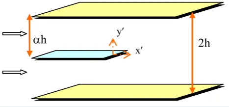
In this paper, we consider the steady, two-dimensional flow of incompressible viscous fluid that constitutes the merging flow in which two oncoming channel flows are forced to join into one. The geometry of problem consists of an infinite long straight channel |y′|≤h, −∞ < x′ < ∞ of width 2h containing a disposed straight splitter plate placed at y′ = αh, −1 < α < 1 within the channel as shown inFigure 1.
Here (x′, y′) represent dimensional rectangular coordinates. The position of splitter is controlled by a splitter position parameter α. If α= 0 then the splitter plate will coincide with the x-axis while the plate will lie above and below the x-axis if α> 0 and α< 0 respectively. The inlet and outlet boundary flow assumed to be same as the plane Poiseuille flow appropriate to the single width channel for downstream while double channels for up-stream of splitter. Although for symmetric case, the various attempts had been made by several authors for ex-ample; [2] [7]-[13] yet owing to the complexity for asymmetric flow which resembles actually to the real life problems, unfortunately due attention was not given.
Obviously a question arises how does our study differ with previous attempts? Following are few facts which cover the answer of this question.
We consider non-uniform rectangular meshing while they used mostly square grid.
We use higher order scheme while previously the authors used mostly 2nd order scheme.
We consider asymmetric flow while previously the symmetric flow cases were examined.
We study the low, moderate, and high Reynolds numbers flow while previous attempts are mostly based ei-ther on low, moderate or high Reynolds number see for example [7].
The main aim of this attempt is to explore all the aspects of the flow behaviour and examine the understand-ing of the complicated features such as boundary layer separation, growth and decay of vortices, reattachment, trailing-edge and leading-edge properties and variation of skin friction on the solid walls and splitter plate for asymmetric case. In addition to this, the flow behaviour is also simulated for various values of Reynolds number
R and splitter position parameter α. We also observe how asymmetric study differs from the previously at-tempted symmetric cases. We examine the variation of eddies when the splitter plate is moved upward or downward within the channel. The extrapolated results obtained are simulated graphically and are compared with those of previously attempted symmetric cases, like [2]. These are given in Section 5. The formulation and basic flow analysis are presented in Section 2 while Sections 3 and 4 contain the detail of numerical scheme so adopted and computational procedure used respectively.
2. Basic Analysis
The continuity and the Navier-Stokes equations for steady flow of incompressible fluid in dimensional form, in the absence of body force are: [2]
0
′ ′
∇ ⋅V = (1)
(
)
2p
[image:2.595.197.431.600.709.2]ρ V′ ′ ′⋅∇ V = −∇ + ∇′ ′ µ ′ ′V (2) where V′ is the fluid velocity vector, ρ is the constant density, µ is the viscosity coefficient, and p′ is the pressure.
The mechanics of the problem under consideration can briefly be stated as; flow is through an infinite length uniform channel with finite width parallel walls. The upstream region is divided into two channels with the help of semi-infinite splitter plate while downstream is flow between two plates without any splitter plate. The walls and splitter are parallel to each other and x-axis. The upstream of splitter plate is separated by 2αh while down-stream is separated by 2h, as shown in Figure 1. Moreover, the flow is being considered as steady, two-dimen- sional, laminar, and asymmetric about x-axis in general. The flow is generated by the uniform pressure gradient analogous to that of plane Poiseuille flow on inlet and outlet flow to preserve the continuity.
On deforming Equations (1)-(2) into vorticity transport equation in dimensionless form by normalizing veloc-ity, space coordinates and vorticity vector by U (main stream velocity), h, and h/U respectively, we will obtain:
0
∇ ⋅ =V (3)
(
)
R V
∇ × ∇ × =ω ∇ × ×ω (4) where ω=
[
0, 0,E]
is the vorticity vector, R the Reynolds number which is equal to the ratio Uh/ν and ν being the kinematic viscosity.If we introduce u andv
y x
ψ ψ
∂ ∂
= = −
∂ ∂ as velocity components in terms of stream function ψ relation into
Equations (3)-(4), we get,
2 E E
E R
y x x y
ψ ψ
∂ ∂ ∂ ∂
∇ = −
∂ ∂ ∂ ∂
(5)
where
2
E= −∇ψ (6) For the geometry of Figure 1the boundary conditions for these equations are given as follows:
(a) No slip at the walls;
i.e. u= =v 0, on all the solid walls and the splitter plate. (7a)
(b)
( )
(
)
(
)
(
)
[
]
( )
(
)
(
)
(
)
[
]
3 2 2 3
3
3
3 2 2 3
3
3
1
i For 0, 2 3 3 2 ,
1
1
12 6 6
1
as 1
ii For 0, 2 3 3 2 ,
1
1
12 6 6
1
y y y y
E y
x
y y y y
E y
α ψ α α α
α
α α
α ψ α α α
α
α α
> → − + + − + −
− → − − − → −∞ −
< → + − + − +
+ → + − + (7b)
(c) 3
1.5y 0.5y E, 3 as y x
ψ → − → → ∞ (7c)
3. Numerical Scheme
To overcome the problem of rate of convergence and stability of the numerical scheme, we adopt the numerical scheme which consists of the following two methods.
The grid size along x and y directions, will be taken by H, K1 respectively, and around a typical internal grid
point
(
x y0, 0)
we adopt the convention that quantities at(
x y0, 0)
,(
x0+H y, 0)
,(
x0,y0+K1)
,(
x0−H y, 0)
,(
x0,y0−K1)
,(
x0+2H y, 0)
,(
x0,y0+2K1)
,(
x0−2H y, 0)
, and(
x0,y0−2K1)
are represented by thesub-scripts 0, 1, 2, 3, 4, 5, 6, 7 and 8 respectively.
3.1. Fourth order Finite-Difference Method
(
1 3 5 7)
(
2 4 6 8)
2 2 1 0 0 2 2 1 1 116 16 16 16
12 12
5 1 1
2
H K
E
H K
ψ ψ ψ ψ ψ ψ ψ ψ
ψ
+ − − + + − −
− + = −
(8)
0 1 0 2 0 3
2 2 2
1
0 4 0 5 0 6
2 2 2
1 1
0 7 0 8 0
2 2 2 2
1 1
4 4 4
8 8 8
3 3 3
4 1 1
8
3 12 12
1 1 5 1 1
0 2
12 12
P E Q E P E
H K H
Q E P E Q E
K H K
P E Q E E
H K H K
+ + + + − + − − + − + − − − − − + = (9) where
(
)
0 6 2 4 8
1
8 8
144
R P
HK ψ ψ ψ ψ
−
= − + − +
and
(
)
0 5 1 3 7
1
8 8
144
R Q
HK ψ ψ ψ ψ
= − + − + .
3.2. Special Finite-Difference Method
In order to approximate linear partial differential equation (6), we employ second order standard central differ-ence formulation at point “0”, we obtain: [15]
1 2 3 4 0 0
2 2 2 2 2 2
1 1 1
1 1 1 1 2 2
E
H ψ K ψ H ψ K ψ H K ψ
+ + + − + = −
(10)
To deal with Equation (5), we split it equation into following two equations as:
(
)
2
2 ,
E E
B A x y x
x
∂ + ∂ = ∂
∂ (11)
(
)
2
2 ,
E E
C A x y
y y
∂ + ∂ = −
∂
∂ (12)
where A is an arbitrary function of x and y while B R and C R .
y x
ψ ψ
∂ ∂
= − =
∂ ∂
Equation (11) is then approximated along the grid line y = y0, over the range x0−H ≤ ≤x x0+H, by
apply-ing a local transformation for E, given as follows:
e F
E=λ − (13)
where
( )
0
1
, d 2
x
x
F =
∫
B t y t.On the introduction of Equation (13), into Equation (11) and approximation of the derivatives involved by 2nd order central differences, we get
(
)
2 2 21 3 0 0 0 0
0
1 1
2
2 4
B
B H A H
x
λ λ+ − λ − ∂ + λ = ∂
(14)
Similarly, Equation (12) is approximated along the grid line x = x0, over the range y0− ≤ ≤k1 y y0+k1, by
e G
E=µ − (15)
where
( )
0 1 , d 2 y y
G=
∫
C x t t.On using Equation (15) into Equation (12), after the similar approximations as above, we shall obtain
(
)
2
2 2 2
2 4 0 0 0 0
2 1 0 1 1 2 2 4 H C
C H A H
y
K µ µ µ µ
∂
+ − − + = −
∂
(16)
On eliminating A0 between Equations (14) and (16), we have
2
2 2 2 2
1 3 0 0 0 2 2 4 0 0 0
1
1 1
2 2 0
4 4
H
E E B H E E C H
K
λ λ+ − − + µ +µ − − =
(17)
In order to express λ and µ back in terms of E, it can be done from the definitions. It is found that e ,Fi eGj
i Ei j Ej
λ = µ = (18)
where i = 1, 3 and j = 2, 4.
Now, we expand above exponential in powers of their arguments and keep the truncation error of order H4
and 2 2
1
H K . After some simplifications under above arguments and using the Taylor’s theorem during calcula-tions, we obtain
[
]
[
]
2 2 2
0 0
1 3 1 3 1 3
0
1
4 8 2
B H B H
H B
E E E E
x
λ λ+ = + ∂ + + + − ∂
(19)
[
]
[
]
2 2
2
0 1 0 1
1
2 4 2 4 2 4
0 1
4 8 2
C K C K
K C
E E E E
y
µ +µ = + ∂∂ + + + −
(20)
On using Equations (19) and (20) into Equation (17), we get
2 2 2 2 2 2
0 0 1 0 0
1 2 2
1 1
2 2 2 2 2 2
0 0 1 0 0
3 2 4
1 1
2 2 2 2
2 0 0 0 2 1 1 1
2 8 8 2
1 1
2 8 8 2
2
2 0
4 4
B H B H H K C C H
E E
K K
B H B H H K C C H
E E
K K
B H C H H E K + + + + + + − + + + − − + + + = (21)
These approximations give rise to an associated matrix that is always diagonally dominant. The present for-mulation was found to work well for all values of Reynolds number R, whereas results could only be obtained for relatively small values of R by using standard central-difference approximations to Equations (5) and (6). Finally the condition for E is required at grid points on the solid walls. Here we use the same approximation as that is originally due to [16] and is given by
[
]
[
]
1 2 3 2 1 2 1 2 1 3 1 1 , 2 3 1 1 , 2 3 1 , 2w a a
w b b
w c c
E E K E E K E E K ψ ψ ψ = − − = − + − = − − (22)
where the subscripts w1, w2 and w3 represent for the value at the approximate boundary points on upper, lower,
and splitter plate respectively while the subscripts a, b and c signify to the internal grid points most immediate to
4. Computational Procedure
This numerical experiment consists of two steps. In the first step, the Equations (10) and (21) are solved itera-tively with respect to the boundary conditions (7) and (22) by SOR-method [17] until the convergence is achieved according to the criterion:
( 1) ( ) 5 ( 1) ( ) 5
0 0 0 0
max Em+ −Em <10 , max− ψ m+ −ψ m <10− (23) In the second step, Equations (8) and (9) are solved numerically with respect to boundary conditions (7) and (22) by SOR-method on using the data obtained from step 1 as an initial estimation. This procedure is repeated until the convergence is attained according to the above criterion (23). The solutions obtained are further extra-polated by Richardson’s extrapolation technique [18].
5. Results and Discussions
Two parameters R and α have a vital role in the general fluid motion. The ranges for R and α are 0 ≤R ≤ 105 and
−1 < α < 1 but, for the purpose of presentation and discussion, we consider R ∈ {1, 10, 100, 500, 1000, 100,000} while α∈ {−0.5, 0, 0.2, 0.5} throughout the study. The numerical calculations are carried out on grid sizes H ∈ {1/20, 1/40, 1/80, 1/160, 1/320} and K1∈ {1/60, 1/120, 1/240, 1/480} and the presented results are
also extrapolated using the Richardson Extrapolation method. In all the cases the infinite length of channel is numerically approximated and is taken as four.
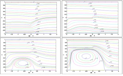
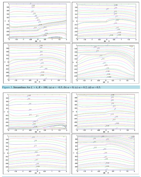
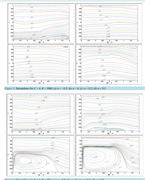
The streamlines for aforementioned R and α are presented in Figures 2-6. These figures depict that the vor-tices are produced in the vicinity of the trailing edge of the splitter plate. The size of eddies increases as α in-creases or if the splitter plate moves upward towards upper plate as shown inFigures 2-6. An interesting situa-tion exists for R = 100,000 and α= 0.5 where whole fluid below the splitter plate is rotating clockwise as shown inFigure 6(d).
[image:6.595.104.525.449.710.2]The trailing edge of the splitter plate needs special attention due to the infinite or singular behaviour of vortic-ity at this point. To deal with this singular point two special treatments are being adopted during calculations for all values of R and α: (i) the method, which is very similar to [7] [8], is used; (ii) the refine meshing is taken in the vicinity of the splitter plate and specially its trailing edge, as shown in Figure 7. More clustering near the singular point is needed as R increases.
Figure 3.Streamlines for L' = 4, R = 100, (a) α = −0.5; (b) α = 0; (c) α = 0.2; (d) α = 0.5.
Figure 4.Streamlines for L' = 4, R = 500, (a) α = −0.5; (b) α = 0; (c) α = 0.2; (d)α = 0.5.
Figure 5. Streamlines for L' =4, R = 1000, (a) α=−0.5; (b) α=0; (c) α=0.2; (d) α=0.5.
Figure 6. Streamlines for L' = 4, R = 105, (a) α= −0.5; (b) α= 0; (c) α= 0.2; (d) α= 0.5.
(
2)
0.5y 3 y as x
ψ → − → ∞
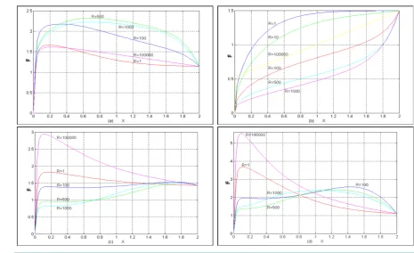
Figure 7. Clustering in the vicinity of splitter plate for different values of α considered. [2] and uα: α= 0 in our case) will be obviously 1.5 for all R. This fact is missing in [2] and this deviation is cor-rected here and is displayed inFigure 8(b). InFigure 8, the distribution for velocity uα along the splitter plate is given for various values of Reynolds number and splitter position parameter. When α= 0 it is observed that the velocity along the splitter increases in downstream of trailing edge of the splitter as we move away from it and curvature of velocity profile increases as R increases. This situation will exist till R = 1000 but it reverses dra-matically when R > 1000 as shown in Figure 6(b). It is noted that the optimum value of velocity lies as x in-creases far from the trailing edge of the splitter, for symmetric case but it is not so for asymmetric case as shown inFigures 6(a)-(d). Moreover, the velocity increases at once after passing the trailing edge for asymmetric case which is clear inFigure 6.
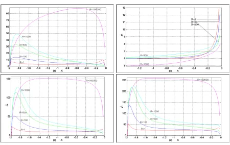
The vortex effects (or in other words the variation of the skin friction) on the upper and lower plates of the channel are also examined here and are displayed in Figure 9andFigure 10 for various values of aforemen-tioned values of R and α. One effect can be noted that the vorticity increases as R increases and it decreases as α increases. These effects occur on both the walls of the channel as shown inFigure 9andFigure 10. Figures 11(a)-(d) depict the variation of dimensionless vorticity on the splitter for various values of R and α, so consi-dered. Figure 11(b) belongs to symmetric flow case and it coincides and compares well with Figure 1 of [2]. This verifies our results. Moreover, the notable thing is that the decay of vorticity to its downstream value takes place over an increasingly longer scale of x as R increases for symmetric case but it is not so for asymmetric one, as shown in Figure 11.
The coefficient of skin friction Cf has vital role in the motion of the fluids and loading-effects on the solid walls. It generally depends upon vorticity, Reynolds number, viscosity, and other geometric aspects. This effect has also been studied here for various values of R and α so considered and its variation with respect to x is also displayed graphically inFigure 12. This figure indicates that the shear stress on the splitter increases as x in- creases and as R decreases. The maximum shear stress will occur at the singular point, which resembles with the physical reality.Figure 12 represents the comparison of our numerical solutions with analytical estimation of
Figure 8. The variation of ucl for various values of R and (a) α= −0.5; (b) α= 0; (c) α= 0.2; (d) α= 0.5.
Figure 9. The variation of wall vorticity on upper plate of channel for various values of R and (a) α= −0.5; (b) α= 0; (c) α= 0.2; (d) α= 0.5.
increases as shown inFigure 12.
Figure 10. The variation of wall vorticity on lower plate of channel for various values of R and (a) α= −0.5; (b) α= 0, (c) α = 0.2; (d) α= 0.5.
[image:11.595.88.539.405.689.2]Figure 12. Comparison of present numerical solution for shear stress on the splitter for symmetric case with analytic solution of [1] (shown here dotted) when (a) R = 1; (b) R = 100; (c) R = 500; (d) R = 1000.
Figure 13. Comparison of present results with analytical results of Badr [1] (here shown as *) for the variation of wall vor-ticity on splitter of channel for various values of R and (a) α= −0.5; (b) α= 0; (c) α= 0.2; (d) α= 0.5.
for the various values of R so considered. The curve with “*” represents the asymptotic solution of while other curves with solid lines belong to our numerical solutions.
References
[1] Sayre, W.W. (1973) Natural Mixing Processes in Rivers. Environmental Impact on Rivers (Ed. Shen Hrech Wen.) Cha 6. Self Published, Fort Collins, CO.
[2] Badr, H., Dennis, S.C.R. and Smith, F.T. (1985) Numerical and Asymptotic Solutions for Merging Flow through a Channel with an Upstream Splitter Plate. Journal of Fluid Mechanics, 156, 63-81.
[image:12.595.138.492.378.563.2][3] Hamblin, P.F. (1980) An analysis of Advective-Diffusion in Branching Channels. Journal of Fluid Mechanics, 99, 101-110. http://dx.doi.org/10.1017/S0022112080000535
[4] William, P.S. (1999) Flow Rate Optimization for the Quadrupole Magnetic Cell Sorter. Analytical Chemistry, 71, 3799-3807. http://dx.doi.org/10.1021/ac990284+
[5] Pedley, T.J. (1980) The Fluid Mechanics of Large Blood Vessel. Cambridge University Press, Cambridge. http://dx.doi.org/10.1017/cbo9780511896996
[6] Sera, T., Sanao, S. and Hirohisa, H. (2005) Respiratory in a Realistic Tracheostenosis Model. Journal of Biomechani-cal Engineering, 125, 461-471. http://dx.doi.org/10.1115/1.1589775
[7] Bramley, J.S. (1982) A Numerical Treatment of Two-Dimensional Flow in a Branching Channel. Lecture Notes in Physics, 170, 155-160. http://dx.doi.org/10.1007/3-540-11948-5_14
[8] Bramley, J.S. (1984) The Numerical Solution of Two-Dimensional Flow in a Branching Channel. Computers & Fluids,
12, 339-355. http://dx.doi.org/10.1016/0045-7930(84)90014-8
[9] Bramley, J.S. (1987) Numerical Solution for Two-Dimensional Flow in a Branching Channel Using Boundary-Fitted Coordinates. Computers & Fluids, 15, 297-311. http://dx.doi.org/10.1016/0045-7930(87)90012-0
[10] Krijger, J.K.B. and Hillen, B. (1990) Steady Two-Dimensional Merging Flow from Two Channels into a Single Chan-nel. Applied Scientific Research, 47, 233-246. http://dx.doi.org/10.1007/BF00418053
[11] Lonsdale, G. and Bramley, J.S. (1988) A Non-Linear Multigrid Algorithm and Boundary-Fitted Coordinates for the Solution of a Two-Dimensional Flow in a Branching Channel. Journal of Computational Physics, 78, 1-14.
http://dx.doi.org/10.1016/0021-9991(88)90034-4
[12] Nakamura, K. and Chiba, K. (1993) Numerical Simulation of Fibre Suspension Flow. Part 1. Merging Flow. Journal of the Textile Machinery, Society of Japan-English Edition, 39, 1-6.
[13] Tsui, Y.Y. and Lu, C.Y. (2005) A Study of the Recirculating Flow in Planar, Symmetrical Branching Channels. Inter-national Journal for Numerical Methods in Fluids, 50, 235-253. http://dx.doi.org/10.1002/fld.1052
[14] Mancera, P.F. and Hunt, R. (1997) Fourth Order Method for Solving the Navier-Stokes Equations in a Constricting Channel. International Journal for Numerical Methods in Fluids, 25, 1119-1135.
http://dx.doi.org/10.1002/(SICI)1097-0363(19971130)25:10<1119::AID-FLD610>3.0.CO;2-4
[15] Dennis, S.C.R. and Smith, F.T. (1980) Steady Flow through a Channel with a Symmetrical Constriction in the Form of Step. Proceedings of the Royal Society of London A, 372, 393-414. http://dx.doi.org/10.1098/rspa.1980.0119
[16] Woods, L.C. (1954) A Note on the Numerical Solutions of Fourth Order Differential Equations. Aeronautical Quar-terly, 5, 176-184.
[17] Hildebrand, F.B. (1978) Introduction to Numerical Analysis. Tata McGraw Hill Publishing Co. Ltd., New Delhi. [18] Jain, M.K. (1997) Numerical Methods for Scientific and Engineering Computation. New Age International (P) Limited,
![Figure 13. Comparison of present results with analytical results of Badr [1] (here shown as *) for the variation of wall vor-ticity on splitter of channel for various values of R and (a) α = −0.5; (b) α = 0; (c) α = 0.2; (d) α = 0.5](https://thumb-us.123doks.com/thumbv2/123dok_us/7961674.753372/12.595.76.528.80.336/figure-comparison-results-analytical-variation-splitter-channel-various.webp)
