Effects of Reducing the Length of the Questionnaire by
Multiple Matrix Sampling on the Validity of Structural
Equation Modeling for Factors Affecting Job Morale
Pimpilai Jaikaew, Suntonrapot Damrongpanit*
Faculty of Education, Chiang Mai University, Chiang Mai, Thailand
Copyright©2018 by authors, all rights reserved. Authors agree that this article remains permanently open access under the terms of the Creative Commons Attribution License 4.0 International License
Abstract
The research was designed to examine theeffects of question setting using different conditions into 10 sets on the validity of structural equation modeling for factors affecting job morale. The data was collected from 690 personnel working in regional Statistical Offices around Thailand by using cluster random sampling. The tool used in collecting data was the questionnaire with 95 items and 5 levels of rating scale. The discrimination value was between 0.244 and 0.860 and the reliability: α was from 0.699 to 0.900. Data analysis was conducted by the use of descriptive statistics and structural equation modeling by Mplus 7.4 program. The findings showed that the structural equation modeling with question setting in 3 sets of sub-questionnaires, cooperated with item sampling without replacement and non-fixing core items, conformed to the empirical data the most and that overall relationship between the structural model parameter and the model parameter from the complete questionnaire was high in a positive way.
Keywords
Multiple Matrix Sampling, StructuralEquation Modeling, Competitive Model, Split Questionnaires, Job Morale
1. Introduction
Structural Equation Modeling or SEM is one of the widely popular statistical techniques used in both behavioral sciences and social sciences [52] due to its two distinguished characteristics. One is that it can be used to analyze the model with latent variable (the variable which is studied with abstract characteristics and cannot be completely measured as it needs the measurement index called “observed variable”) and analyze for the effect at the same time [33]. Another is that it has relaxed assumptions [11] as well as an opportunity for model
modification provided to the researcher in case of incomplete conformation of the model the empirical data [56]. With these two distinguished characteristics;SEM is widely accepted and better applied in current research. This results in obtaining the findings from the research with different forms of problems that frequently revealed the measurement errors in the studied variables, such as Multi level structural equation modeling (MSEM)
(
[4]; [49])
,Multi-group analysis [10], Growth models analysis(
[16]; [60]), Multitrait-Multimethod analysis(
MTMM)
[5], and Meta-Analytic Structural Equation Modeling (MASEM)(
[40]; [55])
, etc. Although SEM provides reliability of the findings, some of its limitations are still found in the model using a great number of both latent and observed variables.of the shorter questionnaire was higher than the longer one. For [39], the team studied the effects of the length of questionnaire on the participation and found that the length resulted to data provision with the statistical significance at .01, so it could be concluded that the length of the questionnaire was one principal factor affecting the measurement variation, besides the limitations regarding incomplete variable measurement of the research in social sciences. Once the conclusion became more explicit, [57] proposed the solution to the length of the tool inorder to reduce the problem by the technique called “Multiple Matrix Sampling: MMS.” This tool was applied to deal with the fault in providing data and measurement variation and to improve the data quality [15].
According to Shoemaker’s concept, several educational institutions appreciated the benefits of MMS. Various forms of international measurement and assessment were applied which were; 1) Trends in International Mathematics and Science Study: TMISS (42]; [45]), 2) Programme for International Student Assessment: PISA which focuses on assessing the students’ capability in applying knowledge and life skills and members in the project are currently from more than 70 countries worldwide [48], 3) Progress in International Reading Literacy Study: PIRLS [42], and 4) National Assessment of Education Progress: NAEP [44]. In addition to the national sectors, there are some other organizations applying MMS, such as economic and political organizations as well as public health sectors [19]. However, there is no empirical evidence that obviously confirms the application of MMS in the social science research, especially the application in measuring SEM affected from the length of the questionnaire.
1.1. Multiple Matrix Sampling
MMS was originally mentioned in the beginning of 1950 by Turnbull, Ebel and Lord, the researchers of the Education Testing Service, who proposed the way to solve the problems found in the educational assessment by using MMS. Later, Lord, Hooke, and Tukey developed statistical procedures to estimate the population’s parameters which MMS was applied [57]. After that, [57] studied this concept and created the textbook about MMS which statistical methodology, estimation, hypothesis testing, and guidelines of MMS application in collecting data were included in the content and widely used afterwards.
The principle of MMS is that items in the complete questionnaire are divided into sub-questionnaires [50] and each of the sub-questionnaires is managed to be in use for collecting data from each group of the responders [59]. The two main rules are to be considered. The first rule is the principle in indicating the number of the item set which [57] explained that it should be considered from; 1) the number of the sub-questionnaires (t) (no higher than the fewest items used in measuring the variables of the conceptual
framework), 2) the number of responders answering the sub-questionnaires (n) (considered from total number of the responders (N) divided by the number of the sub-questionnaires (t)), and 3) the number of items in the sub-questionnaires (k) (considered from total number of items (I) divided by the number of the sub-questionnaires (t)). For example, there are 300 items (I=300) in the complete questionnaire and the number of the fewest items in the variable is 3 when there are 900 participants (N=900). The researcher can design the division of the sub-questionnaires into two options. That means the sub-questionnaires can be divided into 3 sets of 100 items (t=3, k=100) and there are 300 responders for each set, or the sub-questionnaires are divided into 2 sets of 150 items (t=2, k=150) and there are 450 responders for each set (n=450), respectively. The second rule is the principle of item setting which each set of the sub-questionnaires can be arranged in two options. The first option is the use of core items [64] and the second option is item sampling with replacement which refers to repeated items or item sampling without replacement which refers to randomized items [9]. Practically, in case that the number of items in each sub-questionnaire is not equal after dividing the sub-questionnaires, there are two steps to deal with the fraction of the items; the set number of the sub-questionnaires is firstly sampled, and then the items are sampled into the sub-questionnaires (in case of item sampling with replacement) or the rest of the items is managed into the set (in case of item sampling without replacement). For instance, there are 5 items for measuring the variable and the researcher divides the sub-questionnaires into 2 sets and uses item sampling without replacement. Consequently, each set contains different numbers of items including one of 2 items and the other of 3 items, and then the researcher manages with the item no. 3 by sampling the set of sub-questionnaires before adding it into the selected one.
1.2. The Hypothetical Model
construct job morale. [34] also mentioned about basic factors influencing job morale. [38] stated that there were 3 needs within an individual which were generated from learning in society, culture, and environment and developed into those three needs of each individual. [63] viewed that an individual developed his self-confidence from 4 elements comprising self-awareness, consideration, satisfaction, and action after decision and [18] divided 10 elements influencing job satisfaction which included job security, job advancement, management satisfaction, wage and salary, job description, command or supervision, communication, work environment, and other fringe benefits. It is clear that all concepts are related to constructing job morale and it has been used as the foundation in various fields of studying human behaviors.
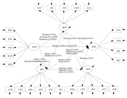
In synthesizing the variables from the previous approaches, 5 latent variables are revealed which are 1) Job Morale: JMO (state of mind and emotions affecting job concentration)measured from 4 observed variables including Company Policy and Administration: CPA, Administration: ADS, Superiors Subordinates Peeves: SSP, and Security: SEC, 2) Job Motivation: MOT (factors stimulating or leading individuals to an attempt to be energetic to achieve the job targets) measured from 5 observed variables including Energetic: EGT, Job Security: JSE, Esteem: EST, Egoistic Needs: EGN, and
Self-actualization: SAC, 3) Self Confidence: SCD (the personnel’s ability to perform their duties to achieve the job targets) measured from 5 observed variables including Emotional Stability: EMS, Courage: COU, Self-Reliance: SRT, Autonomy: AUT, Adaptability: ADP, 4) Job Satisfaction of officers: SFO (positive emotions or attitude towards the job) measured from 6 observed variables including Achievement: ACH, Control Over Work Itself: CWI, Responsibility: RES, Advancement: ADV, Job Cognition: JCO, and Job Action Tendency: JAT, and the last latent variable is Work Environment: WEN (things and conditions around the employees) measured from 5 observed variables including Readiness Factor: REF, Interpersonal relations: INR, Atmosphere environment: TEN, Management: MAN, and Social and Fringe benefits: SFB, respectively. However, these variables are so abstract that it could not define behaviors that directly represent job morale, or that the amount could not be calculated. The researcher, therefore, had an idea to develop SEM of factors affecting job morale by applying MMS in question setting with different conditions and study the results against the harmonized index. Hence, details of the results, showing the link between the variables according to the hypothesis and the data sources supporting the relationships of the variables in SEM, are explained in the form of hypothesis model as shown in Figure 1.
[image:3.595.83.511.402.732.2]2. Materials and Methods
2.1. Research Design
The researcher aimed to study the forms of item sampling and examine the effects of using each data set from 10 sets of questions in different conditions into on the conformity of structural equation modeling and empirical data between the model using the data from complete questionnaire and that from sub-questionnaire. The previous findings by [23], [36], [28], and [54] enabled the researcher to expect that 3 sets of questions provided better harmonized index than that from 2 sets, and that the index than that from complete questionnaire, respectively. The reason was that the complete questionnaire was divided into several sub-questionnaires resulting in fewer items per set, better cooperation in answering the questions from the
responders, and better harmonized index having the questionnaire with more items per set. For the approach by [9], the researcher expected that item sampling without replacement provided better harmonized index than sampling with replacement.
2.2. Research Sample
[image:4.595.86.511.318.698.2]According to the hypothesis model, there were 63 parameters to be estimated in SEM when 10 samples were fixed for 1 parameter ([20]; [29]) and 630 responders were needed. After data collection, it was found that there were totally 690 responders and that the number was higher than the estimation and was enough for parameter estimation. The responders were consisted of 149 government servants (21%), 336 government employees (49%), and 205 mission-based employees (30%).
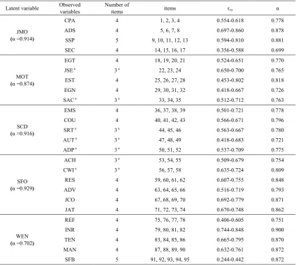
Table 1. Structure of measuring variables and quality of the questionnaire
Latent variable Observed variables Number of items items rxy α
JMO
(α =0.914)
CPA 4 1, 2, 3, 4 0.554-0.618 0.778
ADS 4 5, 6, 7, 8 0.697-0.860 0.878
SSP 5 9, 10, 11, 12, 13 0.594-0.810 0.881
SEC 4 14, 15, 16, 17 0.356-0.588 0.699
MOT
(α =0.874)
EGT 4 18, 19, 20, 21 0.524-0.651 0.770
JSE a 3 a 22, 23, 24 0.650-0.700 0.765
EST 4 25, 26, 27, 28 0.453-0.802 0.818
EGN 4 29, 30, 31, 32 0.418-0.667 0.726
SAC a 3 a 33, 34, 35 0.512-0.712 0.763
SCD
(α =0.916)
EMS 4 36, 37, 38, 39 0.501-0.721 0.778
COU 4 40, 41, 42, 43 0.566-0.671 0.796
SRT a 3 a 44, 45, 46 0.563-0.667 0.780
AUT a 3 a 47, 48, 49 0.418-0.683 0.721
ADP a 3 a 50, 51, 52 0.537-0.709 0.775
SFO
(α =0.929)
ACH 3 a 53, 54, 55 0.509-0.679 0.754
CWI a 3 a 56, 57, 58 0.635-0.724 0.809
RES 4 59, 60, 61, 62 0.607-0.755 0.848
ADV 4 63, 64, 65, 66 0.516-0.719 0.793
JCO 4 67, 68, 69, 70 0.692-0.779 0.871
JAT 4 71, 72, 73, 74 0.670-0.748 0.862
WEN
(α =0.702)
REF 4 75, 76, 77, 78 0.406-0.605 0.751
INR 4 79, 80, 81, 82 0.744-0.848 0.900
TEN 4 83, 84, 85, 86 0.665-0.795 0.870
MAN 4 87, 88, 89, 90 0.632-0.761 0.872
SFB 5 91, 92, 93, 94, 95 0.244-0.442 0.872
2.3. Research Instrument and Procedure
The tool used in this research was the questionnaire containing 95 items with 5 levels of rating scale and covering the measurement of hypothesis model consisting of 5 latent variables. Each of the questions was examined for content validity by the expert before the try-out on 100 government servants, government employees, and mission-based employees working in provincial statistic offices who were not in the sampled group. The aim was to calculate discrimination values by Item-total Correlation (rxy) and reliability (α) using Cronbach’s
Alpha Coefficient. When examining the tool quality, it revealed that each of the latent and observed variables contained high level of confidence at 0.699 - 0.900, especially the variables- JMO, MOT, SCD, and SFO which possessed similar values. However, it was noticed that WEN was the variable with a little lower value than others. The highest number of items used to measure the latent variables was 22 (for SFO) and the lowest number of items was 17 (for JMO and SCD), whereas the lowest number of items used to measure the observed variables was found in 6 variables as shown in Table 1. The personnel provided the data by considering each of the questions and mark in the box to express their level of agreement/ (from 5 = the most to 1 = the least). The length of time used for collecting data lasted 2 weeks and 100% of receiving data from the questionnaire.
2.4. Data Analysis
The researcher recorded all results from the complete questionnaire into the computer and calculated the average of each observed variable as shown in Table 1 consequently, there were 25 values found (from 25 observed variables) and were used in the analysis in order to examine data features by descriptive statistics and consider the relationship between the observed variables Pearson Product Moment Correlation Coefficient
(
as shown in Table 6.) before conducting an analysis for answering the research goal using the program Mplus 7.4 [43].In the analysis to answer the research goal, the researcher divided the process into two stages as follows.
In the first stage, it was comparison of the competitive model that used the data from 10 models of sub-questionnaires. The df values of models were all equal in this stage, so the researcher only considered the Chi-Square difference when the model with the lowest Chi-Square was the best [3] in the group under conditions. After that, the model was adjusted and analyzed to define the harmonized index in the next stage.
In the second stage, it was model modification for which the researcher selected and the original model that used the data from complete questionnaire. The researcher adjusted the model until it reached the criteria of consistency by considering the index used in examining
the goodness of fit statistics which were Relative chi-squareor degree of freedom containing the value less than 2 [56] and the p-value representing statistical insignificance at .05
(
p < .05)
. Additionally, it was necessary to consider Comparative Fit Index(
CFI)
and Tucker-Lewis Index(
TLI)
which should not be higher than0.90(
if it was higher than 0.95, it showed very good conformity), whereas the index of Root Mean Square Error of Approximation(
RMSEA) and the index of Standardized Root Mean Square Residual(
SRMR)
should be lower than 0.08(
if it was higher than 0.05, it showed very good conformity) [30]. In the estimation of parameter value, the maximum likelihood was applied because the researcher observed that the data was shown in normal distribution[56].3. Findings
3.1. Result of Question Setting
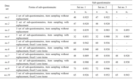
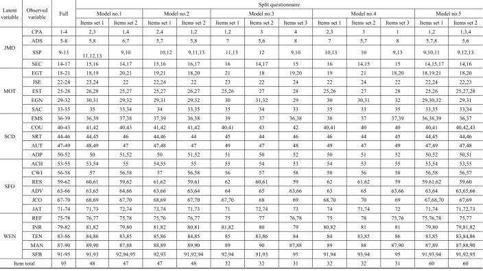
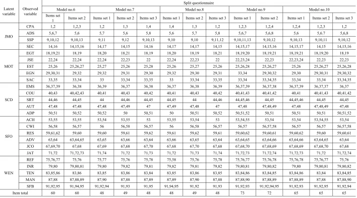
From the previously mentioned principle of MMS, when considering all 95 items according to the conceptual framework (indicated as the original model), the researcher could design the set of questions into 10 models based on two reasons. The first reason was that the complete questionnaire used in data collection contained 6 observed variables and used 3 questions to measure the variables. If the researcher sampled the items without replacement, it was able to arrange the items in the maximum number of 3 sets and the items in each set were not repeated. The second reason was that the researcher considered the use of core items which either 1 item or 2 items was possible. However, 3 core items could not be used because some observed variables were measured with the fewest items of 3. As a result, if the 3 core items were used, all 3 sets of sub-questionnaires would contain the same items. Criterion for item setting was in 10 possible models as shown in Table 2 and item setting based on the criterion was shown in Table 7.
Practically, the researcher noticed that there were some items in model no.2, model no.4, model no.6, and model no.8, were not sampled in the item sampling to measure the variables with replacement. On the other hand, the sampling without replacement revealed that all items were sampled to measure the variables in the models. Some variables were measured with 4 items, but there were 3 sets of sub-questionnaires, such as model no. 3, had 1 item as fraction which was later sampled to be included in the sub-questionnaires together with other items under the same definitions in measuring variables, and then calculated the average in the process of data management.
noticed that , overall, the α value of the sub questionnaire in each model was similar.
3.2. Effects of Item Setting on the Consistency of the Structural Equation Modeling
3.2.1. Comparison of the Harmonized Index of Item Setting Based on Different Criteria
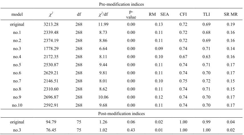
According to the results of examining the validity of SEM by considering the harmonized indices between the use of the data from complete questionnaire and the use of data from sub-questionnaires, overall harmonized indices of both original model and competitive model revealed that all 11 models did not meet the standard. For the original model, χ2 was 3213.276
(
with statisticalsignificance
)
, df value was 268, and the relative chi-square was 11.990. For the competitive model, χ2was in a range from 1778.289 to 2696.872
(
without statistical significance)
, df value was 268, RMSEA was between 0.090 and 0.115, CFI was between 0.670 and 0.750, TLI was between 0.630 and 0.721, and SRMR was between 0.138 and 0.190. Moreover, the researcher noticed that the index of relative chi-square for each model was obviously distinguished which the value was between 6.635 and 10.063. This showed that each model had different goodness of fit statistics as shown in Table 3, as for Pre-modification indices.In addition, the researcher had an observation by comparing the relative chi-square values of the models from item setting between 2 sets and 3 sets obtained from 5 pairs of the models which were model no.1 and model no.3, model no.2 and model no.4, model no.5 and model
no.7, model no.6 and model no.8, and model no.9 and model no.10. It was found that the models from the item setting in 3 sets provided a lower relative chi-square value than that of 2 sets and the researcher chose the model no.3
(
3 sets of sub-questionnaires, item sampling without replacement)
to be the competitive model and original model in the model modification afterwards.3.2.2. Comparison of the Harmony in the Competitive Model
The researcher modified the original model and the model no.3 and compared the harmonized index of SEM. After the modification, it revealed that the harmonized index with empirical data met the criteria when both models had a different indices of χ2
(
94.789 and76.446)
,equal degree of freedom
(
df=75)
, and different p-values(
0.061 and 0.432. The relative chi-square indicated that the harmony of the model no.3 was better than that of the original model and the detailed information was in Table 3. while Post-modification indices and the primary data of the model measurement were shown in the Appendix.Moreover, the researcher considered the detailed information of the competitive model parameters between the original model and the model no.3 after the model modification. It was figured out that the factor loading of all 25 observed variables in both models was positive and different from zero at the statistical significance at 0.01. Also, the observation on the observed variables in the original model showed that the factor loading values of 10 variables were higher while those of 10 variables were lower than those of the model no.3, respectively as shown in Figure 2.
Table 2. Reliability of the sub-questionnaire in different criteriafor data setting
Data
set Forms of sub-questionnaire
Sub-questionnaire
Set no. 1 Set no.2 Set no.3
n α1 n α2 n α3
no.1 2 set of sub-questionnaires, item sampling without replacement 48 0.925 47 0.922 - -
no.2 2 set of sub-questionnaires, item sampling with replacement 47 0.928 48 0.920 - -
no.3 3 set of sub-questionnaires, item sampling without replacement 32 0.839 32 0.903 31 0.893
no.4 3 set of sub-questionnaires, item sampling with replacement 32 0.851 32 0.908 31 0.885
no.5 2 set of sub-questionnaires, item sampling without replacement, fixed 1 core items 60 0.942 60 0.936 - -
no.6 2 set of sub-questionnaires, item sampling with replacement, fixed 1 core items 60 0.940 60 0.938 - -
no.7 3 set of sub-questionnaires, item sampling without replacement, fixed 1 core items 48 0.889 49 0.938 48 0.928
no.8 3 set of sub-questionnaires, item sampling with replacement, fixed 1 core items 48 0.900 49 0.939 48 0.930
no.9 2 set of sub-questionnaires, item sampling without replacement, fixed 2 core items 73 0.951 72 0.946 - -
no.10 3 set of sub-questionnaires, item sampling without replacement, fixed 2 core items 65 0.926 65 0.952 65 0.943
[image:6.595.86.516.487.740.2]Table 3. Harmonized indices of structural equation modeling with empirical data between the data from both complete questionnaire and sub-questionnaires
Pre-modification indices
model χ2 df χ2/df p-
value RM SEA CFI TLI SR MR
original 3213.28 268 11.99 0.00 0.13 0.72 0.69 0.19
no.1 2339.48 268 8.73 0.00 0.11 0.72 0.68 0.16
no.2 2374.19 268 8.86 0.00 0.11 0.72 0.69 0.16
no.3 1778.29 268 6.64 0.00 0.09 0.74 0.71 0.14
no.4 2172.35 268 8.11 0.00 0.10 0.67 0.63 0.16
no.5 2530.87 268 9.44 0.00 0.11 0.74 0.71 0.17
no.6 2629.21 268 9.81 0.00 0.11 0.74 0.70 0.17
no.7 2146.51 268 8.01 0.00 0.10 0.75 0.72 0.15
no.8 2310.60 268 8.62 0.00 0.11 0.74 0.71 0.15
no.9 2696.87 268 10.06 0.00 0.12 0.74 0.70 0.17
no.10 2592.91 268 9.68 0.00 0.11 0.74 0.70 0.17
Post-modification indices
original 94.79 75 1.26 0.06 0.02 1.00 0.99 0.04
no.3 76.45 75 1.02 0.43 0.01 1.00 1.00 0.02
The consideration regarding the relationship of factors affecting job morale in the original model showed the factor, which directly influenced job morale and differed from zero in a positive way with the statistical significance at 0.01, was work environment (WEN) with the effect value of 0.607, except job motivation
(
MOT)
, self-confidence(
SCD)
, and job satisfaction (SFO), which had no direct effect. Besides the direct effect estimation, the consideration of the total effect (TE) from the sum between direct effect (DE) and indirect effect (IE) found that the factor affecting job morale most was work environment (WEN) due to a higher standardized total effect than other factors (β= 0.806) which the ratio was three times more likely to be direct effect than indirect effect. Additionally, the following factor was job motivation (MOT) which the ratio between direct effect and indirect effect was nearly the same, whereas self-confidence (SCD) had only direct effect and job satisfaction (SFO) was likely to be negative in case of direct effect, but positive in case of indirect effect.For the model no.3, the factor which directly influenced job morale was work environment (WEN) as same as that of the original model because it was only one factor with the effect different from zero in a positive way with the statistical significance at 0.01, whereas job motivation
(
MOT)
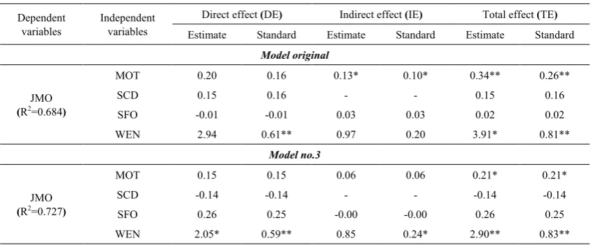
showed the effect different from zero in a positive way with the statistical significance at 0.05 which the ratio was twice more likely to be direct effect than indirect effect. Additionally, self-confidence (SCD) had only direct effect in a negative way and job satisfaction (SFO) was likely to be negative in case of indirect effect, but obviously positive in case of direct effect. [image:7.595.84.513.101.338.2]Note: 1)** with statistical significance at .01, * with statistical significance at .05; 2) order of parameters: original model / model no.3; 3) R2: Coefficient of determination
Table 4. Summary of effects of variables affecting job morale
Dependent
variables Independent variables
Direct effect (DE) Indirect effect (IE) Total effect (TE)
Estimate Standard Estimate Standard Estimate Standard Model original
JMO
(R2=0.684)
MOT 0.20 0.16 0.13* 0.10* 0.34** 0.26**
SCD 0.15 0.16 - - 0.15 0.16
SFO -0.01 -0.01 0.03 0.03 0.02 0.02
WEN 2.94 0.61** 0.97 0.20 3.91* 0.81**
Model no.3
JMO
(R2=0.727)
MOT 0.15 0.15 0.06 0.06 0.21* 0.21*
SCD -0.14 -0.14 - - -0.14 -0.14
SFO 0.26 0.25 -0.00 -0.00 0.26 0.25
WEN 2.05* 0.59** 0.85 0.24* 2.90** 0.83**
In addition, when considering the coefficient of determination from the analyses of both models, it was found that the model no.3 showed 0.730 while the original model showed 0.680 which was a little lower than that of the model no.3. When the result from the analysis of each parameter in the model was calculated for the relative chi-square by Pearson’s Product Moment correlation: rxy,
it resulted in 0.800, showing that both models provided the estimation result into the same direction at a rather high level and the details of effect value estimation were shown in Table 4.
4. Conclusions and Recommendations
The findings revealed that 3 sets of question setting provided better harmonized index than that in 2 sets of item sampling, whereas 2 sets of item sampling provided better index of consistency than that in the complete questionnaire. These findings conformed to the hypothesis and the researcher expected that there were two important causes to be explained.
The first cause is that question setting in 3 sets of sub-questionnaires reduced the number of items per set as well as a decrease in number of pages which were fewer than the question setting in 2 sets of sub-questionnaires; meanwhile, the setting in 2 sets of sub-questionnaires reduced the number of items per set as well as a decrease in number of pages which were fewer than that of the complete questionnaire, respectively. When it was used in collecting data, it helped the responders pay more attention to answering the questions, and reduce boredom, fatigue, responder’s burden [59], the variation caused by answering too many items in the questionnaire [57]. The discoveries by [66]confirmed that the rate of responding to the questionnaire might significantly reduce when the length of the questionnaire was more than 4 pages and it might result to the quality of the collected data
(
[27]; [32])
. Additionally, several researchers who studied the effect of the response rate mentioned that the effect value mightreduce if a very long questionnaire was used in data collecting
(
[1]; [35]; [2])
. Meanwhile, several researchers compared the rates of response between the use of long and short questionnaires and found that the responders prefer the shorter questionnaire to the longer one(
[7]; [8]; [26]; [31]. Consequently, it was suggested that the questionnaire should be divided into more than 2 sets if the researchers required the use of a lot of questions in collecting data according to the advice proposed by [23].each component of each sub-questionnaire, there should be at least 1 core item that the responders had to answer altogether. However, the comparison of the index values, between the model using no core item and the model using core item, showed that the model using no core item provided a better harmonized index. It might be from the reason that the use of core item led to an increase in the number of questions per set which conformed to the research of [58] who conducted a study on the effect caused by the questionnaire with a lot of questions and the result was measured in response rate showing that the rate reduced when there were too many questions.
Although the researcher adjusted the model until the harmonized index met the criteria, there was an observation that some parameters of both models were still negative and the cause might possibly be from low reliability. When the researcher arranged the questions based on the criteria, it affected the balance in distributing questions and the average in measuring each sub-questionnaire. The findings required the researcher to be careful in indicating model specification which was a very important step or it could be considered “the heart or key” of SEM analysis because it was a process related to theories, research, and information technology used in developing the models and examining the quality of the tool before collecting and analyzing the data in order to make it the most accurate in measuring the model. However, all parameters had the harmony at 80% when the rest of 20% might be caused by the variation in measuring the variables due the use of many variables in SEM. These findings conformed to the research by [59] indicating that the confidence and predictive validity of both the complete questionnaire and the shortened questionnaire were similar.
In the viewpoints of the researcher regarding the question setting by MMS, it seemed that the method was another option that the researcher could select to be used in setting the questions in order to make it more
convenient and quicker when collecting data as well as generating the responders’ motivation. However, the approach used for MMS was not clear enough as there were no theorists mentioning the principles of question setting about a proper number of sets or core items used and the distribution of effect values resulted from item sampling with or without replacement. If the researcher applied the method, it was necessary to indicate the form of question setting suitable for the data in order to obtain accurate research result and to make it more reliable afterwards. To generate the tool, the researcher could use negative questions distributed in the end of the questionnaire in order to examine the willingness and concentration in providing the data by considering all the questions. There might be additional study on the effect of gender on the variables as well as the study on the effect of the way of life among people living in each region to find out if it affected the variables or not because each region had its own different social and cultural contexts to be used in others, such as multi-group analysis, factor analysis, multi-level analysis, or even growth models analysis owing to the fact that obtaining the hypothesis model for these analyses needed to be thoroughly synthesized based on the theories as same as SEM.
Acknowledgements
Appendix
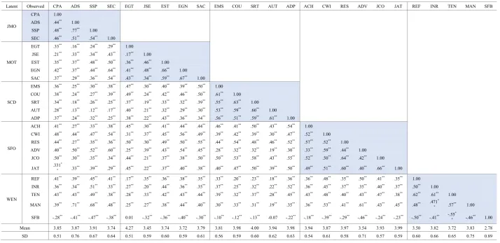
Table 5. Correlation coefficient between variables (model original)
Latent Observed CPA ADS SSP SEC EGT JSE EST EGN SAC EMS COU SRT AUT ADP ACH CWI RES ADV JCO JAT REF INR TEN MAN SFB
JMO
CPA 1.00 ADS .44** 1.00
SSP .48** .77** 1.00 SEC .46** .51** .54** 1.00
MOT
EGT .33** .16** .24** .29** 1.00 JSE .21** .33** .34** .43** .17** 1.00 EST .35** .37** .48** .50** .36** .46** 1.00 EGN .42** .37** .44** .64** .41** .48** .66** 1.00 SAC .37** .29** .36** .54** .43** .34** .59** .67** 1.00
SCD
EMS .36** .25** .30** .38** .47** .30** .40** .39** .50** 1.00 COU .38** .24** .27** .39** .49** .24** .42** .46** .50** .61** 1.00 SRT .34** .18** .26** .25** .37** .19** .33** .32** .39** .55** .63** 1.00 AUT .28** .13** .12** .17** .40** .21** .32** .29** .30** .53** .59** .60** 1.00 ADP .37** .24** .32** .25** .38** .22** .43** .36** .34** .56** .51** .59** .61** 1.00
SFO
ACH .41** .27** .33** .38** .45** .30** .41** .44** .44** .46** .41** .50** .43** .54** 1.00 CWI .48** .44** .47** .54** .31** .37** .45** .56** .49** .39** .42** .39** .30** .47** .52** 1.00 RES .44** .27** .35** .36** .50** .30** .49** .50** .55** .44** .54** .48** .46** .52** .57** .52** 1.00 ADV .40** .50** .52** .60** .25** .39** .43** .54** .45** .28** .32** .32** .19** .30** .33** .59** .44** 1.00
JCO .50** .30** .35** .34** .44** .21** .37** .38** .50** .50** .53** .58** .43** .55** .52** .50** .64** .42** 1.00
JAT .331** .33** .39** .29** .45** .22** .37** .40** .38** .40** .47** .50** .39** .50** .49** .51** .60** .40** .66** 1.00
WEN
REF .41** .39** .45** .41** .17** .35** .36** .38** .35** .33** .20** .23** .18** .36** .36** .48** .35** .50** .41** .35** 1.00 INR .36** .34** .51** .33** .27** .20** .44** .36** .35** .37** .25** .32** .22** .52** .36** .45** .37** .35** .40** .37** .50** 1.00 TEN .43** .43** .49** .38** .28** .33** .42** .43** .44** .39** .32** .37** .28** .45** .43** .48** .40** .43** .47** .38** .62** .61** 1.00
MAN .39** .71** .68** .48** .25** .27** .38** .44** .40** .30** .33** .31** .19** .35** .36** .53** .41** .61** .43** .45** .48** .471*
* .57** 1.00
SFB -.28** -.41** -.47** -.38** 0.01 -.32** -.36** -.40** -.30** -.10** -.12** -.13** -0.07 -.22** -.18** -.39** -.29** -.46** -.24** -.23** -.50** -.41** -.55*
* -.46** 1.00
Mean 3.85 3.87 3.91 3.74 4.27 3.45 3.74 3.72 3.79 3.81 3.98 4.00 3.94 3.98 3.94 3.87 3.97 3.54 3.93 3.99 3.50 3.82 3.72 3.83 2.78 SD 0.51 0.76 0.67 0.64 0.51 0.59 0.60 0.59 0.61 0.56 0.59 0.60 0.62 0.63 0.54 0.61 0.58 0.71 0.57 0.59 0.60 0.66 0.65 0.75 0.89
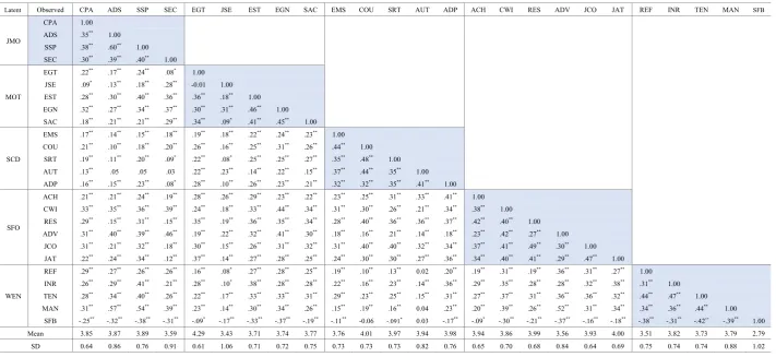
Table 6. Correlation coefficient between variables (model no.3)
Latent Observed CPA ADS SSP SEC EGT JSE EST EGN SAC EMS COU SRT AUT ADP ACH CWI RES ADV JCO JAT REF INR TEN MAN SFB
JMO
CPA 1.00 ADS .35** 1.00
SSP .38** .60** 1.00 SEC .30** .39** .40** 1.00
MOT
EGT .22** .17** .24** .08* 1.00 JSE .09* .13** .18** .28** -0.01 1.00 EST .28** .30** .40** .36** .36** .18** 1.00 EGN .32** .27** .34** .37** .30** .31** .46** 1.00 SAC .18** .21** .21** .29** .34** .09* .41** .45** 1.00
SCD
EMS .17** .14** .15** .18** .19** .18** .22** .24** .23** 1.00 COU .21** .10** .18** .20** .26** .16** .25** .31** .26** .44** 1.00 SRT .19** .11** .20** .09* .22** .08* .25** .25** .27** .35** .48** 1.00 AUT .13** .05 .05 .03 .22** .23** .14** .22** .15** .37** .44** .35** 1.00 ADP .16** .15** .23** .08* .28** .10** .26** .23** .21** .32** .32** .35** .41** 1.00
SFO
ACH .21** .21** .24** .19** .28** .26** .29** .23** .22** .23** .25** .31** .33** .41** 1.00 CWI .33** .35** .36** .39** .24** .18** .33** .44** .34** .31** .30** .26** .21** .34** .38** 1.00 RES .29** .15** .31** .15** .35** .19** .36** .35** .34** .28** .40** .36** .36** .37** .42** .40** 1.00 ADV .31** .40** .39** .46** .19** .22** .32** .41** .30** .18** .16** .21** .14** .18** .23** .42** .27** 1.00
JCO .31** .21** .32** .18** .30** .15** .26** .31** .32** .31** .40** .40** .32** .34** .37** .41** .49** .30** 1.00 JAT .22** .24** .34** .12** .37** .14** .27** .28** .25** .24** .30** .30** .27** .36** .34** .40** .41** .29** .47** 1.00
WEN
REF .29** .27** .26** .26** .16** .08* .27** .28** .25** .19** .10** .13** 0.02 .20** .19** .31** .19** .36** .31** .27** 1.00 INR .26** .29** .41** .21** .28** .10* .38** .28** .28** .22** .16** .23** .14** .36** .29** .35** .28** .28** .32** .38** .31** 1.00 TEN .28** .34** .40** .26** .22** .17** .33** .33** .31** .29** .23** .25** .15** .31** .27** .37** .31** .36** .36** .32** .44** .47** 1.00 MAN .31** .57** .54** .39** .23** .14** .30** .34** .26** .15** .19** .16** 0.04 .23** .20** .39** .26** .52** .31** .34** .34** .36** .44** 1.00
SFB -.25** -.32** -.38** -.31** -.09* -.17** -.33** -.37** -.19** -.11** -0.06 -.091* 0.03 -.17** -.09* -.30** -.21** -.37** -.16** -.18** -.38** -.31** -.42** -.39** 1.00 Mean 3.85 3.87 3.89 3.59 4.29 3.43 3.71 3.74 3.77 3.76 4.01 3.97 3.94 3.98 3.94 3.86 3.99 3.56 3.93 4.00 3.51 3.82 3.73 3.79 2.79 SD 0.64 0.86 0.76 0.91 0.61 1.06 0.71 0.72 0.75 0.73 0.73 0.73 0.82 0.76 0.65 0.70 0.68 0.84 0.64 0.69 0.75 0.74 0.74 0.88 1.02
Table 7. Item setting according to different conditions
Latent
variable Observed variable Full
Split questionnaire
Model no.1 Model no.2 Model no.3 Model no.4 Model no.5
Items set 1 Items set 2 Items set 1 Items set 2 Items set 1 Items set 2 Items set 3 Items set 1 Items set 2 Items set 3 Items set 1 Items set 2
JMO
CPA 1-4 2,3 1,4 2,4 1,2 1,2 3 4 2,3 3 1 1,2 1,3,4
ADS 5-8 5,8 6,7 5,7 5,8 7 5,6 8 7 5,7 8 5,7,8 5,6
SSP 9-13 11,12,13 9,10 10,12 9,11,13 11,13 12 9,10 10,13 10 9,13 9,10,11 9,12,13
SEC 14-17 15,16 14,17 15,16 16,17 16 14,17 15 16 14,15 15 14,15,17 14,16
MOT
EGT 18-21 18,19 20,21 19,21 18,20 21 18 19,20 19 21 18,20 18,19,21 18,20
JSE 22-24 23,24 22 22,24 22 23 22 24 22 24 22 22,24 22,23
EST 25-28 26,28 25,27 25,27 26,27 25,26 27 28 25,26 27 28 25,26 25,27,28
EGN 29-32 30,31 29,32 29,31 29,32 30 31,32 29 30 30,31 32 29,30,32 29,31
SAC 33-35 35 33,34 34 33,35 35 34 33 35 33 35 33,35 33,34
SCD
EMS 36-39 36,39 37,38 37,39 36,38 39 37 36,38 38 37 37,39 36,38,39 36,37
COU 40-43 41,42 40,43 41,42 41,42 40,41 43 42 40,41 40 40 40,41 40,42,43
SRT 44-46 44,45 46 44,46 44 45 44 46 46 44 45 44,45 44,46
AUT 47-49 48,49 47 47,48 47 49 47 48 49 47 49 47,49 47,48
ADP 50-52 50 51,52 50 51,52 51 50 52 50 51 52 50,52 50,51
SFO
ACH 53-55 53,54 55 54,55 55 55 54 53 54 53 55 53,54 53,55
CWI 56-58 57 56,58 57 56,58 56 57 58 58 56 58 56,58 56,57
RES 59-62 60,61 59,62 61,62 59,61 62 60,61 59 62 61,62 59 59,61,62 59,60
ADV 63-66 63,65 64,66 63,66 63,64 64 65 63,66 63 65 63,66 63,64 63,65,66
JCO 67-70 68,69 67,70 68,69 67,70 67,70 68 69 68,70 70 69 67,68,70 67,69
JAT 71-74 71,73 72,74 73,74 71,73 71 72,74 73 74 71,74 72 71,74 71,72,73
WEN
REF 75-78 76,77 75,78 75,76 76,77 75 77 76,78 75 78 75,76 75,76,78 75,77
INR 79-82 81,82 79,80 81,82 80,81 81,82 80 79 80,82 81 81 79,80 79,81,82
TEN 83-86 84,86 83,85 85,86 84,85 85 83,86 84 84 83,85 86 83,85 83,84,86
MAN 87-90 89,90 87,88 88,89 89,90 89 90 87,88 89 88 87,90 87,89 87,88,90
SFB 91-95 91,93 92,94,95 92,93 91,92,94 92,94 91,93 95 91,94 93,94 95 91,93,94 91,92,95
Table 7. Item setting according to different conditions (continued)
Latent
variable Observed variable
Split questionnaire
Model no.6 Model no.7 Model no.8 Model no.9 Model no.10
Items set
1 Items set 2 Items set 1 Items set 2 Items set 3 Items set 1 Items set 2 Items set 3 Items set 1 Items set 2 Items set 1 Items set 2 Items set 3
JMO
CPA 1,2 1,2,3 1,2 1,3 1,4 1,4 1,3 1,2 1,2,3 1,2,4 1,2,4 1,2,3 1,2
ADS 5,6,7 5,6 5,7 5,6 5,8 5,6 5,7 5,8 5,6,7 5,6,8 5,6 5,6.7 5,6,8
SSP 9,10,12 9,10,13 9,11 9,12 9,10,13 9,10 9,10 9,11,12 9,10,11,13 9,10,12 9,10,13 9,10,11 9,10,12
SEC 14,16 14,15,16 14,17 14,15 14,16 14,17 14,17 14,15 14,15,17 14,15,16 14,15,17 14,15 14,15,16
MOT
EGT 18,19,21 18,19 18,20 18,21 18,19 18,20 18,19 18,21 18,19,20 18,19,21 18,19,21 18,19,20 18,19
JSE 22,24 22,24 22,24 22,23 22 22,24 22,23 22 22,23,24 22,23 22,23,24 22,23 22,23
EST 25,26 25,26,27 25,27 25,26 25,28 25,26 25,27 25,26 25,26,28 25,26,27 25,26 25,26,27 25,26,28
EGN 29,30,31 29,32 29,32 29,31 29,30 29,32 29,30 29,31 33,34 29,30,32 29,30 29,30,31 29,30,32
SAC 33,35 33,34 33 33,34 33,35 33 33,34 33,35 33,34 33,34,35 33,34 33,34 33,34,35
SCD
EMS 36,37,39 36,38 36,39 36,37 36,38 36,37 36,38 36,39 36,37,39 36,37,38 36,37,39 36,37,37 36,37
COU 40,43 40,42,43 40,41 40,43 40,42 40,41 40,43 40,42 40,41,43 40,41,42 40,41 40,41,43 40,41,42
SRT 44,46 44,45 44 44,46 44,45 44,45 44 44,46 44,45,46 44,45 44,45,46 44,45 44,45
AUT 47,48 47,48 47,48 47,49 47 47,49 47,48 47 47,48 47,48,49 47,48 47,48,49 47,48
ADP 50,51 50,52 50,52 50 50,51 50 50,51 50,52 50,51,52 50,51 50,51 50,51 50,51,52
SFO
ACH 53,55 53,55 53,54 53,55 53 53,55 53,54 53 53,54,55 53,54 53,54 53,54,55 53,54
CWI 56,58 56,57 56 56,58 56,57 56 56,58 56,57 56,57 56,57,58 56,57 56,57 56,57,58
RES 59,61,62 59,60 59,60 59,61 59,62 59,61 59,62 59,61 59,60,62 59,60,61 59,60,62 59,60 59,60,61
ADV 63,64 63,64,65 63,65 63,66 63,64 63,66 63,65 63,64 63,64,65 63,64,66 63,64,66 63,64,65 63,64
JCO 67,69,70 67,68 67,69 67,68 67,70 67,68 67,70 67,68 67,68,70 67,68,69 67,68,69 67,68,70 67,68
JAT 71,72 71,72,73 71,74 71,72 71,73 71,72 71,73 71,74 71,72,73 71,72,74 71,72,73 71,72 71,72,74
WEN
REF 75,76,77 75,76 75,77 75,76 75,78 75,58 75,76 75,78 75,76,77 75,76,78 75,76,78 75,76,77 75,76
INR 79,80 79,80,81 79,80 79,82 79,81 79,82 79,81 79,82 79,80,81 79,80,82 79,80 79,80,81 79,80,82
TEN 83,85,86 83,86 83,85 83,86 83,84 83,85 83,86 83,85 83,84,86 83,84,85 83,84,86 83,84 83,84,85
MAN 87,88 87,88,89 87,90 87,88 87,89 87,89 87,90 87,88 87,88,90 87,88,89 87,88,89 87,88 87,88,90
SFB 91,92,95 91,94,95 91,92,94 91,93 91,95 91,94,95 91,92 91,93 91,92,93 91,92,94,95 91,92,93 91,92,95 91,92,94
REFERENCES
[1] Adams, L. M., & Darwin, G. (1982). Solving the quandary between questionnaire length and response rate in educational research. Research in Higher Education, 17, 231–40.
[2] Bogen, K. (1996). The Effect of Questionnaire Length on Response Rates – A Review of the Literature. Proceedings of the Section on Survey Research Methods, American Statistical Association, 1020–1025.
[3] Bollen, K. A. (1989). Structural equations with latent variables. NY: John Wiley & Sons.
[4] Bryne, B. M.
(
2012)
. Structural Equation Modeling with Mplus: Basic Concepts, Applications and Programming. NY: Routledge.[5] Chaidi, T., & Damrongpanit, S. (2016). Development and validity testing of belief measurement model in Buddhism for junior high school students at Chiang Rai Buddhist Scripture School: An application for Multitrait-Multimethod analysis. Educational Research and Reviews, 11(18), 1731-1740
[6] Chen, F., Bollen, K. A., Paxton, P., Curran, P., & Kirby, J. (2001). Improper solutions in structural equation models: Causes, consequences, and strategies. Sociological Methods & Research, 29, 468-508.
[7] Chlan, L. L.
(
2004)
. Relationship between two anxiety instruments in patients receiving mechanical ventilatory support. J Adv Nurs, 48, 493–499.[8] Coast, J., Flynn, T. N., & Salisbury, C.
(
2006)
. Maximising responses to discrete choice experiments: a randomised trial. Appl Health Econ Health Policy, 5, 249-260.[9] Cochran, W. G. (1977). Sampling Techniques (3rd ed.).
NY: Wiley.
[10] Damrongpanit, S. (2014). An interaction of learning and teaching styles influencing mathematic achievements of ninth-grade students: A multilevel approach. Educational Research and Reviews, 9(19): 771-779.
[11] Diamantopoulos, A., &Siguaw, J. A.
(
2000).
Introducing LISREL: A Guide for the uninitiated. London: Sage Publication.[12] Dillman, D. A., Sinclair, M. D., & Clark, J. R. (1993). Effects of questionnaire length, respondent-friendly design, and a difficult question on response rates for occupant-addressed census mail surveys. Public Opinion Quarterly, 57, 289−304.
[13] Evans, L.
(
1997)
. Understanding teacher morale and job satisfaction. Teaching and teacher education, 13(
8)
, 831-845.[14] Fallah, N.
(
2014)
. Willingness to communicate in English, communication self-confidence, motivation, shyness and teacher immediacy among Iranian English-major undergraduates: A structural equation modeling approach. Learning and Individual Differences, 30, 140-147.[15] Feray, A., & Michel, W.
(
2005)
. Split Questionnaire Design. Michigan Ross School of Business.[16] Filipiak, K., & Klein, D.
(
2017)
. Estimation of parameters under a generalized growth curve model. Journal of Multivariate Analysis, 158, 73-86.[17] Fox, R. J., Crask, M. R., & Kim, J.
(
1988)
. Mail survey response rate, A meta-analysis of selected techniques for including response. The Public Opinion Quarterly, 52, 467-491.[18] Gilmer, B. V. H.
(
1967)
. Applied Psychology. NY: Mc Grow Hill.[19] Gonzalez, J. M. & Eltinge, J. L. (2007). Multiple matrix sampling: A review. Proceedings of The Section on Survey Research Methods, American Statistical Association, 3069–3075.
[20] Hair, J. F., Black, W. C., Babin, B. J., & Anderson, R. E.
(
2010)
. Multivariate data analysis: A global perspective.(
7th ed).
NJ: Pearson Education Inc.[21] Hedlund, A., Ateg, M., Andersson, I. M., & Rosen, G.
(
2010)
. Assessing motivation for work environment improvements: Internal consistency, reliability and factorial structure. Journal of Safety Research, 41(
2)
, 145-151. [22] Herzberg, F., Mausner, B., & Synderman, B. B. (1959). TheMotivation to work. NY: John Willey & Sons.
[23] Herzog, R. A., & Bachman J. G. (1981). Effects of questionnaire length on response quality. The Public Opinion Quarterly, 45(4), 549-559.
[24] Hoffman, S. C., Burke, A. E. & Helzlsouer K. J.
(
1998)
. Controlled trial of the effect of length, incentives, and follow-up techniques on response to a mailed questionnaire. Am Journal Epidemiol.148, 1007–1011.[25] Jacky, C. K. C., Daniel, Y. T., Jessica, J. T., Kan, P. G., & Joshua, H.
(
2015)
. The Chinese student satisfaction and self-confidence scale is reliable and valid. Clinical Simulation in Nursing, 11(
5)
, 278-283.[26] Jenkinson, C., Coulter, A., & Reeves, R.
(
2003)
. Properties of the Picker Patient Experience questionnaire in a randomized controlled trial of long versus short form survey instruments. Journal Public Health Med, 25, 197–201. [27] Johnson, W. R., Sieveking, N. A., & Clanton, E. S. (1974).Effects of Alternative Positioning of Open-Ended Questions in Multiple-Choice Questionnaires. Journal of Applied Psychology, 59, 776–778.
[28] Kalantar, J. S., & Talley, N. J.
(
1999)
. The effects of lottery incentive and length of questionnaire on health survey response rates: a randomized study. J Clin Epidemiol, 52, 1117-1122.[29] Kelloway, E. K.
(
1998)
. Using LISREL for Structural equation modeling: A researcher’s Guide. Thousand Oaks: Sage Publication.[30] Kelloway, E. K.
(
2015)
. Using Mplus for Structural equation modeling: A researcher’s Guide(
2nd ed.)
. CA:Sage Publication.
patients randomly drawn from the Pennsylvania Cancer Registry: a randomized trial of incentive and length effects. BMC Med Res Methodol, 10, 65.
[32] Kraut, A. I., Wolfson, A. D., & Rothenberg, A. (1975). Some Effects of Position on Opinion Survey Items. Journal of Applied Pyschology, 60, 774–776.
[33] Lei, P. W. & Wu, Q.
(
2007)
. Introduction to structural equation modeling: Issues and practical considerations. Educational Measurement: Issues and Pactice. Fall. 33-43. [34] Locke, E. A. (1976). The Nature and Causes of JobSatisfaction. In: Dunnette, M.D., Ed., Handbook of Industrial and Organizational Psychology, 1, 1297-1343. [35] Love, L. T. & Turner, A. G. (1975). The Census Bureau
Experience: Respondent Availability and Response Rates. Proceedings of the Business and Economics Section, American Statistical Association, 76–85.
[36] Lund, E. & Gram, I. T.
(
1998)
. Response rate according to title and length of questionnaire. Scand J Soc Med, 26, 154– 160.[37] Maslow, A. H.
(
1970)
. Motivation and Personality. NY: Harper and Row Publishers.[38] McClelland, D. C. (1961). The Achieving Society. Princeton, NJ: D. Van Nostrand Company.
[39] Mond, J.M., Rodgers, B., Hay, P. J., Owen, C., & Beumont, P. J. V.
(
2004)
, Mode of delivery, but not questionnaires length, affected response in an epidemiological study of eating-disordered behavior. Journal of Clinical Epidemiology, 57(
11)
, 1167-1171.[40] Montazemi, A. R., & Saremi, H. Q.
(
2015)
. Factor affecting adoption of online banking: A meta-analytic structural equation modeling study. Information & Management, 52(
2)
, 210-226.[41] Mullis, I., Kennedy, A., Martin, M., & Sainsbury, M.
(
2006)
. PIRLS assessment framework and specifications. Chestnut Hill, MA: Boston College.[42] Mullis, I., Martin, M., Ruddock, G., O’Sullivan, C., Arora, A., & Erberber, E.
(
2005).
TIMSS 2007 assessment framework. Chestnut Hill, MA: Boston College.[43] Muthén, L. K., & Muthén, B. O. (2017). Mplus User’s Guide
(
8th ed.)
.
Los Angeles, CA: Muthén & Muthén.[44] National Center for Education Statistics.
(
2010)
. About NAEP. Retrieved from http://nces.ed.gov/ nationsreportcard/about/[45] Neidorf, T., & Garden, R.
(
2004)
. Developing the TIMSS 2003 mathematics and science assessments and scoring guides. In M. O. Martin, I. V. S. Mullis, & S. J. Chrostowski(
Eds.)
, TIMSS 2003 technical report(
pp. 23-66)
. Chestnut Hill, MA : Boston College.[46] Noorizan, M. M., Nur, F. A., Norfazlina, A. Z., & Sharidatul, A.
(
2016)
. The moderating effects of motivation on work environment and training transfer: A preliminary analysis. Procedia Economics and Finance, 37, 158-163.[47] Ordonez, O., Carlos, J., Friederike, S., & Bernd, R.
(
2015)
. Promoting self-confidence, motivation and sustainablelearning skills in basic education. Procedia Social and Behavioral Sciences, 171, 982-986.
[48] Organization for Economic Co-operation and Development
(
OECD)
.(
2006).
Assessing scientific, mathematical, and reading literacy: A framework for PISA 2006. Paris: Author.[49] Pohl, S., & Galletta, M.
(
2017)
. The role of supervisor emotional support on individual job satisfaction: A multilevel analysis. Applied Nursing Research, 33, 61-66. [50] Raghunathan, T. E., & Grizzle, J. E. (1995). A splitquestionnaire survey design. Journal of the American Statistical Association, 90, 54–63.
[51] Rao, J. N. K., Hartley, H. O., & Cochran, W. G.
(
1962)
. On a simple procedure of unequal probability sampling without replacement. Journal of the Royal Statistical Society, 24(
2)
, 482-491.[52] Raykov, Tenko & Marcoulides, G.A.
(
2006)
. A first course in structural equation modeling(
2nd ed.).
NJ : Lawrence Erlbaum Associates, Inc.[53] Raziq, A., & Maulabakhsh, R.
(
2015)
. Impact of working environment on job satisfaction. Procedia Economics and Finance, 23, 717-725.[54] Ronckers, C., Land, C., & Hayes, R.
(
2004)
. Factors impacting questionnaire response in a Dutch retrospective cohort study. Ann Epidemiol, 14, 66–72.[55] Rosopa, P. J., & Kim, B.
(
2017)
. Robustness of statistical inferences using linear models with meta-analytic correlation matrices. Human Resource Management Review, 27(
1)
, 216-236.[56] Schumacker, R. E. & Lomax, R. G.
(
2010)
. A Beginer’s Guide to Structural Equation Modeling(
3rd ed.).
NY: Routledge.[57] Shoemaker, D. M.
(
1973).
Principles and Procedures of Multiple Matrix Sampling. Cambridge: Mass Ballinger. [58] Sindre, R., John, A., & Anna, R.(
2011)
. Response Burdenand Questionnaire Length: Is Shorter Better? A Review and Meta-analysis. Value in health,14
(
8)
, 1101-1108.[59] Smits, N., & Vorst, H. C. M.
(
2007)
. Reducing the length of questionnaires through structurally incomplete design: An illustration. Learning and Individual Differences, 17(
4)
, 25-34.[60] Song, G., & Chang, H.
(
2016)
. Equalities of various estimators in the general growth curve model and the restricted growth curve model. Journal of Statistical Planning and Inference, 169, 88-100.[61] Stanton, J. M., Sinar, E. F., Balzer, W. K., & Smith, P. C. (2002). Issues and strategies for reducing the length of self-report scales. Personnel Psychology, 55, 167−193. [62] Suttikun, C., Chang, H. J., & Bicksler.
(
2017)
. Aqualitative exploration of day spa therapists’ work motivations and job satisfaction. Journal of Hospitality and Tourism Management, 34, 1-10.
[63] Symonds, A. F.
(
1964)
. Teaching Yourself Personality[64] Thomas, N., Raghunathan, T. E., Schenker, N., Katzoff, M. J., & Johnson, C. L. (2006). An evaluation of matrix sampling methods using data from the national health and nutrition examination survey. Survey Methodology, 32, 217–31.
[65] Victor, C. R.
(
1988)
. Some methodological aspects of using postal questionnaires with the elderly. Arch Gerontol Geriatr, 7, 163–72.[66] Yammarino, F. J., Skinner, S. J., & Childers, T. L.
(
1991)
.Understanding mail survey response behavior: A meta-analysis. Public Opinion Quarterly, 55, 613-639. [67] Yu, J., & Cooper, H.
(
1983)
. A quantitative review ofresearch design effects on response rate to questionnaires. Journal of Marketing Research, 20(1), 36-44.