Comparison of Fractional Order PID Controller and
Sliding Mode Controller with Computational
Tuning Algorithm
Chong Chee Soon
1, Rozaimi Ghazali
1,*, Shin Horng Chong
1, Chai Mau Shern
1,
Yahaya Md Sam
2, Ahmad Anas Yusof
31
Centre for Robotics and Industrial Automation, Faculty of Electrical Engineering, Universiti Teknikal Malaysia Melaka, Malaysia 2Department of Control and Mechatronics Engineering, School of Electrical Engineering, Universiti Teknologi Malaysia, Malaysia
3Faculty of Mechanical Engineering, Universiti Teknikal Malaysia Melaka, Malaysia
Copyright©2019 by authors, all rights reserved. Authors agree that this article remains permanently open access under the terms of the Creative Commons Attribution License 4.0 International License
Abstract The industry processes involving punching,
lifting, and digging usually require high precision, high force and long operating hours that increase the prestige in the usage of the electrohydraulic actuator (EHA) system. These processes with the companion of the EHA system usually possess high dynamic complexities that are hard to be controlled and require well-designed and powerful control system. Therefore, this paper will involve the examination of the designed controllers which is applied to the EHA system. Firstly, the conventional proportional-integral-derivative (PID) controller which is the famous controller in the industry is designed. Then, the improved PID controller, which is known as the fractional order PID (FO-PID) controller is designed. After that, the design of the gradually famous robust controller in the education field, which is the sliding mode controller (SMC) is performed. Since the controller’s parameters are essentially influencing the performance of the controller, the meta-heuristic optimization method, which is the particle swarm optimization (PSO) tuning method is applied. The variation in the system’s parameter is applied to evaluate the performance of the designed controllers. Referring to the outcome analysis, the increment of 59.3% is obtained in the comparison between PID and FOPID, while the increment of 67.13% is obtained in the comparison of the PID with the SMC controller. As a conclusion, all of the controllers perform differently associated with their own advantages and disadvantages.Keywords
Electro-Hydraulic, Fractional Order PID, Sliding Mode Control, Robustness Analysis, Particle Swarm Optimization1. Introduction
An actuator requires energy sources in its dynamic responses which are commonly the composition of current, air, or fluid, that is also known as electric, pneumatic, or hydraulic. Practically, each of the energy sources has its own strength and weakness. The capabilities in generating high torque, high power, and accurate positioning tracking with fast motion make the hydraulic power to be extensively utilized in the industry fields. Recently, the hydraulic system with the combination of the electronic devices, which is known as electro-hydraulic actuator (EHA) system has been gradually increased.
Commonly, the dynamics delivered to the different mechanisms are either linear or rotary, which are also referred to the cylinder or motor. Widespread engineering applications dealing with these dynamics have been found in construction, agriculture, oil and gas, mining and material handling machinery. As reported by [1], the construction and agriculture applications occupied the most in the components unit sales by 75% among the other applications in 2014.
The physical modelling of the EHA system usually begins with the power supply, servo-valve, and hydraulic actuator, taking into account the nonlinearities and the related dynamics [2]. The nonlinearities usually exist in the practical system. The sources of the nonlinearities including actuator friction, the mechanism leakages, the compressibility of the fluid, and nonlinear pressure characteristics [3]. These existing issues consequently increase the challenge of the controller design.
Commonly, the uncertain nonlinearities and also the parametric uncertainties are the main uncertainties existing in the EHA system [4, 5]. The uncertain nonlinearities, which are also known as the general uncertainties are the uncertainties that hard to be precisely modelled such as
external disturbances, friction either in the valve or the actuator, and also internal or external leakage. The parametric uncertainties are the changes occurred in the system, including the variation of the mass during the operation, and the changes in the fluid viscosity due to the working temperature and the component wear during the operation. The detailed discussion regarding these uncertainties can be found in [6].
These existing drawbacks consequently motivate researchers and academia to further investigate the effects of these drawbacks, and to design a high-performance control system to minimize the effect of these uncertainties. In this paper, the variation of the supply pressure which represents the EHA system uncertainties is conducted. As has been discussed in [6], the supply pressure is the most influential parameter and playing a vital role in generating the required dynamic and produce a desired motion. Apart of evaluating the performance of the designed proportional-integral-derivative (PID) controller, fractional order PID (FO-PID) controller, and sliding mode controller (SMC), the robustness performance of these controllers can be evaluated through the variation or
changes occurred during the operating condition.
The examination of these controllers and methods in the simulation environment will be applied to the hardware that is in the development process. The organization of this paper is the following. Section 2 is the summary, the inclusion and the exclusion of the paper, followed by the brief explanation of the FO-PID controller in Section 3.1. The derivation of the SMC is presented in Section 3.2. The examination of the controller performance is pictured in Section 4, and finally the conclusion of the study in Section 5.
2. System Modelling
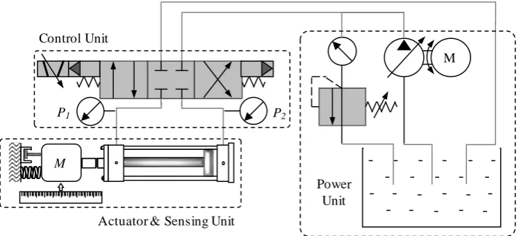
[image:2.595.112.486.365.535.2]Typically, the physical model of the EHA system is composed of control, power, actuator and sensing units as demonstrated in Figure 1. The pipeline was connecting the hydraulic actuator with the servo-valve that will regulate and allowing the oil flow from the chamber to the hydraulic cylinder. The counterforce was generated against the cylinder actuator through the spring and damper that were attached to the mass [7].
Figure 1. Typical units in the EHA system
P1 P2
Control Unit
M
Actuator & Sensing Unit
M
The voltage that supplying the electrical current to the servo-valve coil generating the mechanical motion of the spool-valve. The desired position of the spool-valve was driven from the power source that was fed to the motor with the equation below, which consist of resistance, Rc
and inductance Lc of the coil.
(1) The second-order differential equation was obtained in the servo-valve dynamic, which is related with the motor torque driven from the electrical current as expressed in equation (2), with the servo-valve’s damping ratio, ξ and natural frequency,ω.
(2) The ideal orifice equation of the servo-valve that control the flow, Q has a relation with pressure difference, Pi and
spool-valve displacement, xv in each chamber as:
(3)
(4)
The modelling of the volume with the volume between pipeline and cylinder, Vline in each volume can be expressed
as:
(5) (6) Flow rate, bulk-modulus, and volume that define the pressure, P in each chamber can be expressed as:
(7)
(8)
Total force generated from the hydraulic actuator was obtained through the overall dynamic equation of mass, Mp
spring, Bs, and damper, Ks expressed in the equation (9).
(9)
The parameters of the mathematical model can be obtained in [8]. Also, the discussion regarding the development of the PID controller was carried out in [6]. It is the fact that the practical systems are mostly intrinsically nonlinear, so do the EHA system [9]. In order to overcome
the existing drawback in this system, which is commonly used in the applications for example vehicle part pressing machine, aircraft, and digging machine that required high force and precision, high-performance control system is needed to support the designed system to achieve the desired response.
Therefore, this paper is carried out to verify the improvement that will be generated from the extension of the conventional PID controller, named fractional order PID (FO-PID) controller. The performance analysis between these PID and FOPID controllers will be later compared with the robust SMC controller. Further explanation regarding the development of the SMC will be conducted. In terms of the performance analysis, the robustness examination that was conducted in [6] will be applied.
In a recent trend, the computational tuning algorithm is gradually widespread in different applications. Therefore, the well-known particle swarm optimization (PSO) algorithm will be used to obtain the parameters of each controller. The discussion regarding the PSO algorithm is not covered in this paper and can be found in [6]. The only difference is the changes in the parameters of the PSO algorithm, with the equal parameters applied to each controller during the tuning process. The parameters include the particle’s size (50), the number of iterations (30), the acceleration (2 for both c1 and c2), the inertia
weight (decreased from 0.9 to 0.4) and most important, the performance index that is used to obtain the minimum error, which is the Integral Time Absolute Error (ITAE).
3. Materials and Methods
As emphasized in [9], the hydraulic system is well-known for facing the common unstructured uncertainties issues. These issues consequently increase the difficulties and became the main obstacle in the development of the high performance and high accuracy control system applied in the hydraulic system. Further motivation in the design of the excellent control system is therefore distributed to academia and researchers. In the following Sections, the gradually famous controller, which is the extension of the conventional PID controller, named FOPID controller, and also the robust SMC controller will be discussed.
3.1. Fractional Order PID Controller
In the early 20th century, the fractional order calculus is introduced in [10] which is applied in the control and the dynamic system. By extending the general differential equations into the fractional order differential equations [11], the flexibilities of the fractional order calculus have been employed to the PID controller which yield the Fractional Order (FO-PID) controller.
On the contrary to the three parameters, which are proportional (kp), integral (ki), and derivative (kd) in the
=dl c+ c
V L R I
dt
2
2 2
2 +2ξω +ω = ω
v v
n n n
d x dx
I dt dt 1 1 1 1 1 ; 0, ; 0, − ≥ = − <
v s v
v r v
K x P P x
Q
K x P P x
2 2 2 2 2 ; 0, ; 0, − − ≥ =
− − <
v r v
v s v
K x P P x
Q
K x P P x
1= line+ p( s+ p)
V V A x x
2 = line+ p( s− p)
V V A x x
1
1 ( 1 12 1 )
( )
β
= + + ∫ − − −
line p s p
dV
P Q q q dt
V A x x dt
2
2 ( 2 21 2)
( )
β
= + − ∫ − − −
line p s p
dV
P Q q q dt
V A x x dt
1 2 2 2 ( ) = − = + + + p p p p
p s s p f
F A P P
d x dx
M B K x F
conventional PID controller, two additional parameters which are the integrating order, λ and the derivative order,
μ have been integrated into the integral and derivative gains of the PID controller [11-13]. The transfer function of the conventional PID controller is usually written as
(10)
where Kp is the proportional gain, Ti is the integral gain
time in constant time, and Td is the derivative gain in
constant time. While the additional order that integrated to the FO-PID controller yields the transfer function of
(11)
where the order λ and μ are not necessarily integer numbers [11]. If the order λ and μ are assumed to be 1, the convention PID controller is formed.
The practical system with a fractional order or known as a non-integer type of system can be found in the transmission line or the heat flow system. The closed-loop control system generally consists of an integer or fractional order system with integer or fractional order controller, or the interchangeable of these system and control structure [14].
In the previous study, it is proven that the FO-PID controller, or known as PIλDμ controller is able to improve the conventional PID controller performance with the introduction of the integral and derivation order λ and μ respectively. However, in the computer science point of view, since additional parameters are added to the FO-PID controller, the process to obtain the controller parameters become more complex and simultaneously increase the computational time.
3.2. Sliding Mode Controller
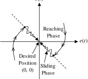
[image:4.595.103.244.607.734.2]Generally, the design of the sliding surface is the most important step in the design of the SMC. Two important properties, which are reaching phase and sliding phase as demonstrated in Figure 2 play vital roles in the varieties of the controller performance.
Figure 2. The basic properties in the design of SMC
The concept of the sliding mode notion was not disseminated in the early 1960s until a book was published by the researcher in [15], and a journal article was written by the researchers in [16]. After that, an insightful view regarding the introduction and the growth of the SMC control strategy has been carried out by [17]. Thereafter, a number of studies regarding the SMC have been proposed to deal with the uncertainties and nonlinearities in the system. The design of the SMC is unique since its performance does not directly depend on the tracking state but is depending on the design of the sliding surface. The concept of the SMC technique is to force the control signal moving toward the sliding surface and force the control signal to stay on that surface once the control signal is reached [18].
Commonly, the general equation of the sliding surface,
s(t) in SMC can be obtained by referring to the system order, n as presented in the following equation.
(12) Referring to the third-order EHA system, the s(t) of the conventional SMC, which is proportional to the error, e
and the control gain, λ can be obtained as
(13) The error produced in a closed-loop environment can be acquired in equation (14) by subtracting the output of the desired tracking with the actual tracking.
(14) The third order linearized EHA system will generate the error with the third derivative as expressed in equation (15).
(15) When the s(t) ≠ 0, switching control, usw will take place
to lead the tracking error from the phase of reaching to sliding. While the s(t) = 0, equivalent control, ueq will
respond to lead the tracking error on s(t) = 0 to the desired point. Thus, the SMC is generally expressed as
(16) The ueq of the SMC will be acquired through the first
derivative of the s(t) as
(17) Some parameters existing in the EHA may be impossible to be gathered and modelled. The simplified EHA model will be employed in the designed controller, where the EHA system will be represented through the perturbed linear model with third order, which has included the disturbances and uncertainties characters as indicated in the following equation.
( ) 1
( ) 1
( )
= + +
= p d
i U s
G s K T s
E s T s
( ) 1
( ) 1
( ) µ λ = + +
= p d
i U s
G s K T s
E s T s
Reaching Phase
Desired Position
(0, 0) Sliding Phase ) (t e ) (t e 1
( ) λ ( )
− = + n d
s t e t
dt
2 ( )=( ) 2+
λ
( )+λ
( )s t e t e t e t
( )= r( )− p( )
e t x t x t
( )= ( )− ( )
e t x tr x tp
( )= ( )+ ( )
smc eq sw
u t u t u t
2 ( )= ( )+2
λ
( )+λ
( )
(18)
where d(t) is composed of the nonlinear leakage and friction, and the external load disturbance. The nominal system parameters are represented in An, Bn, and Cn, while
the uncertainties existed in the un-modelled dynamics are represented by the bounded uncertainties ΔA, ΔB, and ΔC. Then, the third-order EHA system will be organized as
(19) where L(t) is the lumped uncertainties that can be expressed as:
(20) Assuming that L is neglected and substituting equation (15) into (17), the ueq of the SMC will be indicated as
(21) The switching control of the SMC can be acquired by employing the signum function, sign(s) into the sliding surface as expressed in equation (22).
(22) where the signum function has a boundary as expressed in (23), and ks is a positive constant value.
(23)
The Lyapunov theorem as adopted in [19-23] is used to analyse the stability of the controller when s(t) ≠ 0 with the
following function.
(24) The following reaching condition is required to be fulfilled to achieve a stable condition during the tracking from reaching to sliding phase.
for s(t) ≠ 0 (25)
By replacing (15), (16) and (17) into (25), the following
function will be obtained.
(26)
The discontinuous function in equation (22) might leads to the chattering effect, which can be minimized by replacing the hyperbolic tangent function as introduced in [19, 22-23].
(27)
4. Robustness Evaluation
Controllers are playing vital roles especially in the assistant of the engineering processes, for example shifting, shaping and lifting. Apart from being an assistant, the controller is especially useful in dealing with the system major uncertainties and disturbances. It is the fact that the practical systems are mostly intrinsically nonlinear. To overcome the existing drawback in the practical systems, high-performance control system is needed to reduce the actual required elements and achieved the desired response, for example, the voltage or power that generates torque to actuate the load or the application. Apart from reducing the actual effort, the high-performance controller can perform surprisingly in achieving the desired response even with the parameter changes along with the operation.
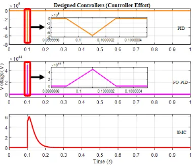
Figure 3 demonstrates the controller effort generated from the designed conventional PID, FO-PID and SMC controllers. Practically, different devices required different limitation according to the size and the structure of that particular system. However, the common practical system has the minimum and maximum voltage of -10 Volts and 10 Volts. As depicted in Figure 3, the conventional PID and FO-PID controllers illustrated the requirement of substantial effort in order to achieve the required response. In terms of energy consumption, the FO-PID controller required the highest energy, which is 44 times of the actual energy. It is followed by the conventional PID controller, which is 5 times of the actual energy. While the SMC controller is outperformed, with the requirement of the energy around 6 Volts to achieve the desired response.
( ) ( ) ( ) ( ) ( ) ( ) ( ) ( ) = − + ∆ − + ∆ + + + ∆ +
p n p n p
n
x t A A x t B B x t
C C u t d t
( )= − ( )− ( )+ ( )+ ( )
x tp A x tnp B x tnp C u tn L t
( )= ±∆ p( )± ∆ p( )± ∆ ( )+ ( )
L t Ax t Bx t Cu t d t
(
2)
1
( )= + + +2λ( )+λ ( )
eq r n p n p
u t x A x B x e t e t
C
( )= ( )
sw s
u t k sign s
1 ; ( ) 0
( ( )) 0 ; ( ) 0
1 ; ( ) 0
> = = − < s t
sign s t s t
s t 2 1 ( ) ( ) 2 =
V t s t
( )= ( ) ( )<0,
V t s t s t
2
( ) ( ) [ ( ) ( ) ( ) ( ( )
( )) 2λ ( ) λ ( )]
= + + −
+ + +
r n p n p n eq
sw
s t s t s x t A x t B x t C u t
u t e t e t
( ) tanh
φ
= sw s sFigure 3. Control effort required to running an EHA system for the PID, FO-PID and SMC controllers
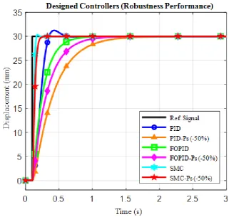
Apart from analysing the performance of the designed controller, robustness of the designed controller is essential, especially in the operation that requires long operating hours. Therefore, the steady-state error, robustness index, and transient response analyses have been carried out to generating numerical data of the designed controllers for the comparison purpose. Based on the numerical data as
Figure 4. Robustness performance for the PID, FO-PID and SMC during the changes of the supply pressure, Ps
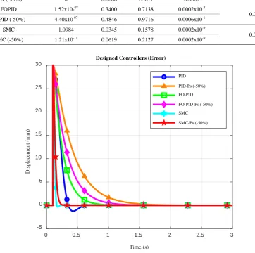
Rise time is an important factor that increases the productivity for example, in the production line that requires lifting process, where the quick processing time is important in the process. Generally, the high-rise time will lead to high overshoot and simultaneously slow down the settling time of the system. In the nominal operating condition tabulated in Table 1, the SMC controller has overcome the former condition which produced the fastest rise time with 0.0345 seconds, fastest settling time with 0.1578 seconds, lowest steady-state error, which is 9 times to the actual value and smallest robustness index value that demonstrate its robustness performance compared to the conventional PID and FO-PID controllers. The
Table 1. Numerical analysis of each controller based on transient, steady-state error and robustness index
Controller Transient Response Steady-state Error (ess)
Robustness Index
OS (%) Tr (s) Ts (s)
PID 4.1160 0.1603 0.5236 0.0005
0.1877
PID (-50%) 0 0.6686 1.3077 0.0007
FOPID 1.52x10-07 0.3400 0.7138 0.0002x10⁻³
0.0764 FOPID (-50%) 4.40x10-07 0.4846 0.9716 0.0006x10⁻¹
SMC 1.0984 0.0345 0.1578 0.0002x10⁻⁹
[image:8.595.105.468.145.505.2]0.0617 SMC (-50%) 1.21x10⁻¹¹ 0.0619 0.2127 0.0002x10⁻⁹
Figure 5. Error generated during the nominal condition and the changes in the supply pressure
Instead of using the conventional tuning techniques, for example, the trial and error, and the Ziegler-Nichols tuning technique, the PSO computational tuning technique, which is very time saving and convenient has been used to acquire the controller’s gains as listed in Table 2.
Table 2. The PSO computational algorithm generated parameters
Controller
Parameter
Kp Ki Kd λ δ
PID 10.0910 0.0013 -4.6985 1 1
FO-PID 34.8991 0.7052 8.5401 2.0296 8.1205
SMC - - - 87.6240 395.7009
0 0.5 1 1.5 2 2.5 3
Time (s)
-5 0 5 10 15 20 25 30
Displacement (mm)
Designed Controllers (Error)
PID PID-Ps (-50%) FO-PID FO-PID-Ps (-50%) SMC
[image:8.595.72.525.589.709.2]5. Conclusions
An EHA system is well-known to be widely applied in various applications, for instance aircraft and vehicle pressing machine. These applications usually involve the processes that demanded high force, high precision, and flexible response which require the assistance of the high-performance control system. However, the high-performance controller designs usually require an expert in the related field. Besides, the cost and the time spend will be the defects in the complex or high-performance controller design. In the industrial field, the PID controller is usually used, which is much easier and simple to be designed. Depending on the required outcome, if the high precision result is required, the PID controller might be unable to achieve the required objective. This paper intends to assess the performance of the common use PID controller, the improved PID controller named fractional order PID controller, and also the SMC controller during the changes of supply pressure in the EHA system. The parameters of each controller are obtained using the PSO tuning algorithm. By referring to the robustness numerical analysis, although the FO-PID controller is capable to outperform the conventional PID controller, with the robustness index value of 0.0764, the robustness index value of the SMC is even smaller which is 0.0617. As the robustness index value represents the error occurred during the changes in the operating condition, the SMC is able to perform better without discarding the important properties of the EHA system during the occurrence of the variation. Apart from using the PSO computational tuning method, the performance of these controllers might be enhanced through different computational tuning methods. Therefore, further investigation regarding the computational tuning algorithm which can be applied in the practical system will be carried out.
Acknowledgements
The support of Universiti Teknikal Malaysia Melaka (UTeM), Universiti Teknologi Malaysia (UTM) and Ministry of Education (MOE) are greatly acknowledged. The research was funded by Short Term Grant No. (PJP/2017/FKE/HI11/S01534), Fundamental Research Grant Scheme (FRGS) Grant No. FRGS/1/2017/TK04/FKE-CERIA/F00333 and Skim Zamalah UTeM.
REFERENCES
[1] L. A. Lynch and B. T. Zigler, “Estimating Energy Consumption of Mobile Fluid Power in the United States,” 2017.
[2] H. E. Merritt, Hydraulic Control Systems. John Wiley & Sons, 1967.
[3] M. Jelali and A. Kroll, Hydraulic Servo-systems: Modelling, Identification and Control. Springer - Verlag London Limited, 2003.
[4] K. Guo, J. Wei, J. Fang, R. Feng, and X. Wang, “Position Tracking Control of Electro-Hydraulic Single-Rod Actuator Based on an Extended Disturbance Observer,” Mechatronics, vol. 27, pp. 47–56, 2015.
[5] Q. Guo, J. Yin, T. Yu, and D. Jiang, “Saturated Adaptive Control of an Electrohydraulic Actuator with Parametric Uncertainty and Load Disturbance,” IEEE Trans. Ind. Electron., vol. 64, no. 10, pp. 7930–7941, 2017.
[6] C. C. Soon, R. Ghazali, H. I. Jaafar, and S. M. Hussein, Syarifah Yuslinda Syed Rozali, “Robustness Analysis of an Optimized Controller via Particle Swarm Algorithm,” Adv. Sci. Lett., vol. 23, no. 11, pp. 11187–11191, 2017.
[7] M. Kalyoncu and M. Haydim, “Mathematical Modelling and Fuzzy Logic based Position Control of an Electrohydraulic Servosystem with Internal Leakage,” Mechatronics, vol. 19, no. 6, pp. 847–858, 2009.
[8] C. C. Soon, R. Ghazali, H. I. Jaafar, and S. Y. S. Hussien, “PID Controller Tuning Optimization using Gradient Descent Technique for an Electro-hydraulic Servo System,” J. Teknol. Sci. Eng., vol. 77, no. 21, pp. 33–39, 2015. [9] J. Yao, Z. Jiao, D. Ma, and L. Yan, “High-accuracy
Tracking Control of Hydraulic Rotary Actuators with Modeling Uncertainties,” IEEE/ASME Trans. Mechatronics, vol. 19, no. 2, pp. 633–641, 2014.
[10] I. Podlubny, “Fractional-Order Systems and PIλDμ-controllers,” IEEE Trans. Automat. Contr., vol. 44, no. 1, pp. 208–214, 1999.
[11] M. Zamani, M. Karimi-Ghartemani, N. Sadati, and M. Parniani, “Design of a Fractional Order PID Controller for an AVR using Particle Swarm Optimization,” Control Eng. Pract., vol. 17, no. 12, pp. 1380–1387, 2009.
[12] I. Podlubny, “Fractional-Order Systems and Fractional-Order Controllers,” Inst. Exp. Physics, Slovak Acad. Sci. Kosice, vol. 12, no. 3, pp. 1–18, 1994.
[13] M. Dulau, A. Gligor, and T.-M. Dulau, “Fractional Order Controllers Versus Integer Order Controllers,” Procedia Eng., vol. 181, pp. 538–545, 2017.
[14] Y. Chen, I. Petras, and D. Xue, “Fractional Order Control - A Tutorial,” in American Control Conference, 2009, 2009, pp. 1397–1411.
[15] U. Itkis, Control Systems of Variable Structure. New York: Halsted Press - John Wiley Sons, Inc., 1976.
[16] V. Utkin, “Variable Structure Systems with Sliding Modes,” IEEE Trans. Automat. Contr., vol. 22, no. 2, pp. 212–222, 1977.
[17] R. A. DeCarlo, S. H. Zak, and G. P. Matthews, “Variable Structure Control of Nonlinear Multivariable Systems: A Tutorial,” Proc. IEEE, vol. 76, no. 3, pp. 212–232, 1988. [18] C. Edwards and S. K. Spurgeon, Sliding Mode Control:
[19] I. Eker and S. A. Akinal, “Sliding mode control with integral augmented sliding surface: design and experimental application to an electromechanical system,” Electr. Eng., vol. 90, no. 3, pp. 189–197, 2008.
[20] M. Mihajlov, V. Nikolic, and D. Antic, “Position Control of an Electro-Hydraulic Servo System using Sliding Mode Control Enhanced by Fuzzy PI Controller,” Facta Univ. Mech. Eng., vol. 1, no. 9, pp. 1217–1230, 2002.
[21] H. M. Chen, J. C. Renn, and J. P. Su, “Sliding mode control with varying boundary layers for an electro-hydraulic position servo system,” Int. J. Adv. Manuf. Technol., vol. 26, no. 1–2, pp. 117–123, 2005.
[22] I. Eker, “Sliding Mode Control with PID Sliding Surface and Experimental Application to an Electromechanical Plant,” ISA Trans., vol. 45, no. 1, pp. 109–118, 2006. [23] I. Eker, “Second-order Sliding Mode Control with