Analysis of robot localisation performance based on Extended Kalman Filter

ANALYSIS OF ROBOT LOCALISATION PERFORMANCE BASED ON EXTENDED KALMAN FILTER

FARAH HAZWANI BINTI CHE HASSAN

A project report submitted in partial

fulfillment of the requirement for the award of the Degree of Master of Electrical Engineering

Faculty of Electrical and Electronic Engineering Universiti Tun Hussein Onn Malaysia

v

ABSTRACT

vi

ABSTRAK

vii

TABLE OF CONTENT

TITLE i

DECLARATION ii

DEDICATION iii

ACKNOWLEGMENT iv

ABSTRACT v

ABSTRAK vi

CONTENT vii

LIST OF TABLES xii

LIST OF FIGURES xiii

LIST OF SYMBOL AND ABBREVIATION xvi

CHAPTER 1 INTRODUCTION 1

1.1 Project Background 1

1.2 Problem Statement 3

1.3 Objective 4

1.4 Scope of Project 4

CHAPTER 2 LITERATURE REVIEW 5

2.1 Introduction 5

viii

2.3 Localisation 6

2.3.1 Types of localisation 7

2.3.1.1 Dead reckoning 7

2.3.1.2 Prior Map Localisation 7

2.3.1.3 Simultaneously Localisation and Mapping (SLAM) 8

2.3.2 Classification of localisation problems 8

2.3.2.1 Position Tracking 8

2.3.2.2 Global Localisation 8

2.3.2.3 Kidnapped robot problem 9

2.4 Mapping 9

2.5 Gaussian Filter 9

2.5.1 Types of Gaussian filter 10

2.5.1.1 Kalman Filter 10

2.5.1.2 Extended Kalman Filter 12

2.5.1.3 Unscented Kalman Filter 15

2.5.1.4 Cubature Kalman Filter 16

2.6 Technology Development 19

2.6.1 Landmark based Navigation of Industrial Mobile Robots 19

2.6.2 Robot Localisation and Kalman Filters 20

2.6.3 Convergence and Consistency Analysis for Extended

Kalman Filter based SLAM 21

2.6.4 LRF based Self Localization of Mobile Robot Using

ix

2.6.5 Navigation of An Autonomous Mobile Robot using EKF

SLAM and Fast SLAM 23

2.6.6 Mobile Robot Position Estimation Using Kalman Filter 24 2.6.7 SLAM using EKF, EH∞ and Mixed E / H∞ Filter 25 2.6.8 Cubature Kalman Filter based Localiation and Mapping 26 2.6.9 A Solution to the Simultaneously Localisation and

Mapping Problem 27

2.6.10 A Slam Algorithm for Indoor Mobile Robot Localisation Extended Kalman Filter and a Segment Based Environment

Mapping 28

2.6.11 Localisation of a Mobile Autonomous Robot Extended

Kalman Filter 28

2.6.12 A Mobile Robot Localisation & Map Building Algorithm &

Simulation 29

CHAPTER 3 METHODOLOGY 35

3.1 Introduction 35

3.2 Flow Chart 36

3.2.1 Flow Chart of The Project 36

3.2.2 The Proposed Flow Chart 37

3.3 Extended Kalman Filter 38

3.3.1 Robot Dimension 38

3.3.2 Process Model 39

x

3.4 Software Development 48

3.4.1 Results Simulation 48

3.4.2 MATLAB Graphical User Interface (GUI) 52

CHAPTER 4 RESULT AND ANALYSIS 56

4.1 Introduction 56

4.2 Analyse the performance of the algorithm using different parameter 57

4.2.1 Result for velocity (1m/s) 57

4.2.2 Result for velocity (3m/s) 58

4.2.3 Result for velocity (5m/s) 59

4.3 Result for Standard Deviation of Distance (m) and Angle (rad) using

Different Velocities 60

4.4 Comparison between of three different methods 62

4.4.1 Result for Kalman Filter Joseph with 45 landmarks 62 4.4.2 Result for Kalman Filter Joseph with 85 landmarks 63 4.4.3 Result for Kalman Filter Joseph with 135 landmarks 64 4.4.4 Result for Kalman Filter Cholesky with 45 landmarks 65 4.4.5 Result for Kalman Filter Cholesky with 85 landmarks 66 4.4.6 Result for Kalman Filter Cholesky with 135 landmarks 67 4.4.7 Result for Kalman Filter Update with 45 landmarks 68 4.4.8 Result for Kalman Filter Update with 85 landmarks 69 4.4.9 Result for Kalman Filter Update with 135 landmarks 70 4.5 Result for Standard Deviation Distance (metre) and Standard

xi

CHAPTER 5 CONCLUSION AND RECOMMENDATION 71

5.1 Conclusion 75

5.2 Recommendation 76

REFERENCES 77

APPENDICES 81

xii

LIST OF TABLE

Table 2.1 Comparison of Gaussian Filter 18

Table 2.2 Previous paper for robot localisation 31

Table 3.1 Extended Kalman filter Algorithm 42

Table 3.2 SLAM Algorithm 42

Table 4.1 Comparison between different velocities 61

xiii

LIST OF FIGURE

Figure 2.1 Model underlying the Kalman Filter 11

Figure 2.2 Typical application of Extended Kalman Filter 13 Figure 2.3 Underlying model of Extended Kalman Filter 13

Figure 2.4 Landmarks and an on board laser scanner 19

Figure 2.5 Robot position 20

Figure 2.6 Measurement model 20

Figure 2.7 Robot movement 22

Figure 2.8 Model of mobile robot platform 22

Figure 2.9 Vehicle coordinate system 23

Figure 2.10 Estimation of the trajectory using EKF with Gaussian Implication 24 Figure 2.11 Trajectory estimation with the Kalman Filter 24 Figure 2.12 Trajectory estimation with the Extended Kalman Filter 25

Figure 2.13 EKF SLAM with low Gaussian noise 25

Figure 2.14 EH∞ SLAM with low Gaussian noise 26

Figure 2.15 E / H∞ Filter SLAM with low Gaussian noise 26 Figure 2.16 Trajectory of the vehicle and landmarks 27 Figure 2.17 The true vehicle path together with surveyed (circles) and

estimated (starred) landmark locations 27

Figure 2.18 Robot sensor position 28

Figure 2.19 Comparison between actual, encoder and Extended Kalman Filter

xiv

Figure 2.20 Mobile robot localisation 29

Figure 2.21 Observation error 30

Figure 2.22 State error 30

Figure 3.1 Flow chart of project 36

Figure 3.2 Flow chart of programming 37

Figure 3.3 Vehicle and observation kinematic 45

Figure 3.4 Open file 49

Figure 3.5 Load data ‘example_webmat.mat’ 49

Figure 3.6 Run ekfslam_sim.m 50

Figure 3.7 Output result 50

Figure 3.8 Code for standard deviation 51

Figure 3.9 Save file as findDist.m ` 51

Figure 3.10 Run simulation findDist.m 52

Figure 3.11 Command window 53

Figure 3.12 GUIDE Quick Start 53

Figure 3.13 GUI Editor 54

Figure 3.14 Save file as simGui.fig 55

Figure 3.15 GUI programmed 55

Figure 3.16 GUI interface 55

Figure 4.1 (a) Movement of robot (1m/s) 57

Figure 4.1 (b) Error for distance and angle (1m/s) 58

Figure 4.2 (a) Movement of robot (3m/s) 58

xv

Figure 4.3 (a) Movement of robot (5m/s) 59

Figure 4.3 (b) Error for distance and angle (5m/s) 60 Figure 4.4 Graph for standard deviation distance (m) versus velocity (m/s) 61 Figure 4.5 Graph for standard deviation angle (m) versus velocity (m/s) 62

Figure 4.6 (a) Movement of robot (45 landmarks) 63

Figure 4.6 (b) Error for distance and angle (45 landmarks) 63

Figure 4.7 (a) Movement of robot (85 landmarks) 64

Figure 4.7 (b) Error for distance and angle (85 landmarks) 64

Figure 4.8 (a) Movement of robot (135 landmarks) 65

Figure 4.8 (b) Error for distance and angle (135 landmarks) 65

Figure 4.9 (a) Movement of robot (45 landmarks) 66

Figure 4.9 (b) Error for distance and angle (45 landmarks) 66

Figure 4.10 (a) Movement of robot (85 landmarks) 67

Figure 4.10 (b) Errors for distance and angle (85 landmarks) 67

Figure 4.11 (a) Movement of robot (135 landmarks) 68

Figure 4.11 (b) Errors for distance and angle (135 landmarks) 68 Figure 4.12 (a) Movement of robot (45 landmarks) 69

Figure 4.13 (a) Movement of robot (85 landmarks) 70

xvi

LIST OF SYMBOL AND ABBREVIATION

KF - Kalman Filter

EKF - Extended Kalman Filter UKF - Unsected Kalman Filter CKF - cubature Kalman Filter GUI - Graphical User Interface GPS - Global Positioning System SD - Standard Deviation

Rad - Radian

1

CHAPTER 1

INTRODUCTION

1.1 Project Background

Generally, robot is a tool of machine that can ease the human burden and can also be classified as an automatic machine where it has the ability to move in a variety of environments according to a predetermined function. Robot serves to replace humans in order of performing tasks that are repetitive and dangerous due to size limitations, and environments that are inconsistent with human life such as in an aerospace, underwater, in the air, underground, or in a space.

2

are harmful to people, property, or itself unless those are part of its design specifications [1].

Mobile robot must capable of moving in any given environment. Besides that, mobile robot must also have the capability of tracking its paths and trajectories in the workspace [2].

In real world, there are methods for locating mobile robot that consists of relative positioning and absolute positioning. For relative positioning, dead reckoning is typically used to calculate the robot positions from a start reference point to the new updated point. As known that dead reckoning is the easier method that is normally used in real time for estimation of the position of a robot using internal sensors. However in the dead reckoning, the position of the robot could not be estimated accurately because it has an unbounded accumulation of errors. Hence, frequent correction is made from other sensors to overcome this problem based on error happened [3]. For absolute positioning depend on the detecting and recognizing of different features in the robot environment.

3

This project studies a navigation algorithm that simultaneously locates of the robots and updates landmarks in a cluttered environment. A key issue being addressed is how to improve the localisation accuracy for mobile robots in a continuous operation in which the Extended Kalman Filter algorithm is adopted to integrate odometry data with sensor to achieve the required robustness and accuracy in the nonlinear dynamical systems. For the sake of simplicity, this project focuses on 2D model and based on the indoor environment to demonstrate the movement of the robot that can localise itself based on the surrounding landmarks.

1.2 Problem Statement

4

1.3 Objective

The main objectives of this project are:

i) To investigate the existing localisation algorithm [30] based on Extended Kalman Filter.

ii) To analyse the performance of the algorithms by using different parameters.

iii) To compare the performance of the algorithms by using several type of update approaches.

1.4 Scope of Project

The scopes of this project are as the following:

i) This project concentrates on robot localisation using surrounding landmarks with Extended Kalman Filter as the estimator.

ii) MATLAB/Simulink is used for modelling the environment and simulation.

5

CHAPTER 2

LITERATURE REVIEW

2.1 Introduction

This chapter describes the prediction of location using surrounding landmark. In this study, SLAM technique is used to estimate the robot location. The first part of this chapter describes the use of landmarks to provide more accurate location.

The second part explains the Kalman filter technique which is used in this project. It is the foundation of the SLAM to solve the problem of localisation of a mobile robot based on the surrounding landmarks and reports its location to the base station.

6

2.2 Landmarks

Landmarks are generally defines as passive objects in the environment that provide a high degree of localisation more accurate that cause by nature or man made use for navigation. Mobile robot that use a landmarks for localisation generally used artificial markers that been use to make localisation easier [4]. Landmarks are distinct features that a robot can recognize from its sensory input. Landmarks can be in geometric shapes which are rectangles, lines and circles and sometimes may include in additional information in form of bar codes. In general, landmarks have a fixed and known position that relative to which a robot can localise itself. Landmarks are carefully chosen to be easy to identify for example there must be sufficient contrast to the background. As usual a robot can use landmarks for navigation in which the characteristics of the landmarks must be known and stored in the robots memory [5].

2.3 Localisation

7

2.3.1 Types of localisation

There are several types of localisation that normally used for solve robot localisation problem such as dead reckoning, prior map localisation and simultaneously localisation and mapping (SLAM).

2.3.1.1 Dead reckoning

Dead reckoning is the process of determining the one present position and the speed from a known past position which is used to predict a future position and speed from a known present position. The dead reckoning position only produces an approximate position because it does not allow for the effect of current or compass error. Dead reckoning helps in determining sunrise and sunset in predicting landfall, sighting lights and predicting arrival times and in evaluating the accuracy of electronic positioning information, [6]. However, the dead reckoning suffers from an accumulation of errors during the operation [3].

2.3.1.2 Prior Map Localisation

8

2.3.1.3 Simultaneously Localisation and Mapping (SLAM)

Localisation is the problem of estimating the robot position includes its path given as known map of the environment. Therefore, the mapping is defined as a construction of the map of the environment knowing the true path of the robot. Simultaneously Localisation and Mapping (SLAM) is the process of building a map of an environment while concurrently generating an estimate for the location of the robot. SLAM provides a mobile robot with a fundamental ability to localise itself and the features in the environment without prior map, which is essential for many navigation tasks [8]. The aim of the SLAM is to recover both the robot path and the environment map using only the data gathered by its sensors. These data are typically the robot displacement estimated from the odometry and features extracted from laser, ultrasonic or camera images.

2.3.2 Classification of localisation problems

There are several problems in robot localisation such as position tracking, global localisation and kidnapped robot problem. Below are the descriptions of these problems.

2.3.2.1 Position Tracking

For position tracking the robot current localisation is updated based on the knowledge of its previous position which is tracking. In this cases supposed to be known the robot initial location. The large position tracking fail to localise the robot if the uncertainly of robot pose is too large [9].

2.3.2.2 Global Localisation

9

2.3.2.3 Kidnapped robot problem

The kidnapped robot problem tackles the case of the robot gets kidnapped and move to another location. The kidnapped robot problem is similar to the global localisation problem only if the robot localise having been kidnapped. The difficulty arises when the robot does not know that it has been moved to another location and it believes it knows where it is but in fact does not. The ability to recover from kidnapped is necessary condition for the operation of any autonomous robot and even more for commercial robots [9].

2.4 Mapping

Map building is a very important issue for a mobile robot to perform tasks autonomously. It is required for the system to simulate the landmark on true map and each landmark should have a features mark to distinguish landmarks in different positions. These landmarks are used to identify in the movement process of mobile robot. These landmarks are observed in the movement process of mobile robot through which independent map is constructed to mark the positions of these landmarks. The problem of robotic mapping is that of acquiring a space model of a robots environment. Maps are commonly used for robot navigation for example localisation. To acquire a map the robots must have a sensors that normally used to observed. Sensors commonly range finders using sonar, laser and infrared technology, radar, compasses and GPS. However, all these sensors are subject to errors often referred to as measurement noise [10].

2.5 Gaussian Filter

10

than the signal. In real time systems a delay is covered because incoming samples need to fill the filter window before the filter can be applied to the signal. The parameter of Gaussian by its mean and covariance is called the moments parameterization because of the mean and covariance are the first and second moments of a probability distribution in which all other moments are zero for normal distributions [11].

2.5.1 Types of Gaussian filter

There are several types of Gaussian Filter that will be discussed in this sub-section including Kalman Filter, Extended Kalman Filter, Unscented Kalman Filter and Cubature Kalman Filter.

2.5.1.1 Kalman Filter

In engineering, filtering is the most important method to reduce the noise from signals. The noisy measurement normally used to estimate a noisy dynamic system based on Kalman Filter technique. Kalman Filter assumes that the action and sensor models are subject to Gaussian noise and assume that the belief can be represented by one Gaussian function. In practice, this might not always be the case but it does allow the Kalman Filter to efficiently make its calculations.

The time or measurement form of the Kalman Filter is expressed in two steps in which the time update of the state variable vector estimate in time that received into the input of the system and created a prediction of the new state. The measurement update adjusts the time update state estimate to take into account measurements that made during the time interval [5].

11

mixed with more noise, generates the visible outputs from the hidden state. The Kalman Filter may be regarded as analogous to the hidden Markov model with the key difference that the hidden state variables are continuous [11]. In order to use the Kalman Filter to estimate the internal state of a process given only a sequence of noise observation one must model the process in accordance with the framework of the Kalman Filter. Fig 2.1 shows model underlying the Kalman Filter [12].

Figure 2.1: Model underlying the Kalman Filter [12]

The Kalman Filter model assumes the true state at time k is evolved from the state at (k-1) according to [12]

(2.1)

is the state transition model which is applied to the previous state

is the control input model which is applied to the control vector

is the process noise which is assumed to be drawn from a zero mean multivariate normal distribution with covariance

at time k an observation (or measurement) of the true state is made according to

12

where is the observation model which maps the true state space into the observed space and is the observation noise which is assumed to be zero mean Gaussian white noise with covariance

(2.3)

the initial state and the noise vectors at each step { are all assumed to be mutually independent. Many real dynamical systems do not exactly fit the model. However, because the Kalman Filter is designed to operate in the presence of noise, an approximate fit is often good enough for the filter to be very useful.

2.5.1.2 Extended Kalman Filter

Unlike Kalman Filter, Extended Kalman Filter (EKF) deals with nonlinear process model and nonlinear observation model which is linear about an estimate of the current mean and covariance as shown in Fig. 2.2. System with nonlinear output maps is treated and the condition needs to ensure the uniform roundedness of the error covariance is related to the observation properties of the underlying nonlinear system. Furthermore, the uniform asymptotic convergence of the observation error is established whenever the nonlinear system satisfies an observation rank condition and the states stay within a convex compact domain.

13

Figure 2.2: Typical application of Extended Kalman Filter

EKF is widely used to estimate current state depends on the discrete time and measurement. At each discrete time step to generate a new state, a nonlinear operator is applied in order to integrate the information from control system and noise. Hence, noise is generated from the hidden, true or state on the Fig. 2.3 according to [11] for the time step k-1, k and k+1. The ellipse represents the multivariate normal distribution for the mean and covariance matrices, the squares represent of the matrices used while for the values represent the vector. The ‘Observed’ represents the measurement of the current state. The ‘Supplied by user’ represents process model and ‘hidden’ represents an actual state of system that is to be estimated by the EKF.

Figure 2.3: Underlying model of Extended Kalman Filter [11] System

Measuring devices System error

source

Control

System state (desired

but not known) Observed

measurement

Optimal estimate of system state Extended

14

The nonlinear process model (from time k to time k + 1) is described as [14]

(2.4)

is the system state (vector) at the time k, k + 1 f is the system transition function

is the control

is the zero mean Gaussian process noise

For state estimate problem, the true system state is not available and needs to be estimated. The initial state is assumed to follow a known Gussian Distribution to estimate the state at each time step by the process model and the

observation. The observation model at time k + 1 is given by

(2.5)

where h is the observation function

is the zero mean Gaussian observation noise

suppose the knowledge on at the time k is

(2.6)

then at time k + 1 follows

(2.7)

where can be computed by the following EKF formula. The predict using process model

(2.8)

15

(2.9)

where is the Jacobian of function f with respect to x evaluated at

The function f can be used to compute the predicted state from the previous estimate and similarly the function h can be used to compute the predicted measurement from the predicted state. However, f and h cannot be applied to the covariance directly. Instead a matrix of partial derivatives which is Jacobian is computed.

2.5.1.3 Unscented Kalman Filter

Unscented Kalman Filter (UKF) is an improvement of the nonlinear EKF. In the UKF, the probability density is approximated by a deterministic sampling of points which represent the underlying distribution as a Gaussian. The nonlinear transformation of these points is intended to be an estimation of the posterior distribution, which can then be derived from the transformed samples. The unscented transformation is a method for calculating the statistics of a random variable which undergoes a nonlinear transformation. The UKF tends to be more robust and more accurate than the EKF in its estimation of error. Consider the following nonlinear system described by the deference equation and the observation model with additive noise [15]

(2.10)

(2.11)

the initial state is a random vector with known mean μo=E[xo] and covariance E[(xo- μo)( . in this case of non additive process and measurement

noise, the unscented transformation scheme is applied to the augmented state.

(2.12)

16

calculate statistic of y, by form a matrix x of 2L + 1 sigma vectors (with corresponding weight ) then can be shown as

(2.13)

√ i (2.14)

√ i-L (2.15)

=λ/(L+λ) (2.16)

=λ/(L+λ) + (1- +β) (2.17)

λ = is a scaling parameter which is set a small value α is spread of the sigma points around

k is secondary scaling parameter which is usually set to 0 β is to incorporate prior knowledge of distribution of x

2.5.1.4 Cubature Kalman Filter

Cubature Kalman Filters (CKFs) is used for the nonlinear dynamic systems with additive process and measurement noise. As is well known, the heart of the Cubature Kalman Filters (CKF) is the third degree spherical radial cubature rule which makes it possible to compute the integrals encountered in nonlinear filtering problems. However, the rule not only requires computing the integration over an n-dimensional spherical region, but also combines the spherical cubature rule with the radial rule, thereby making it difficult to construct higher degree Cubature Kalman Filters (CKFs). Moreover, the cubature formula used to construct the Cubature Kalman Filters (CKF) has some drawbacks in computation. Consider the nonlinear filtering problems with additive process and measurement noise, whose state-space model can be expressed by the pair of difference equations in discrete time [16]

17

(2.19)

Equations (2.18) and (2.19) are the process equation and the measurement equation respectively in which

is the state at time k is the control input

and h are some nonlinear functions is the measurement

and are white noise with zero mean and covariance and and ,

respectively.

Under the Gaussian assumption in the Bayesian filtering framework, the core issue of nonlinear filtering problems is to compute the multi-dimensional weighted integrals whose integrands are all in the form of nonlinear function Gaussian density, viz.

∫ (2.20)

where w( ) = exp( ) is the weighting function and 𝛺 Rn is the region of integration.

18

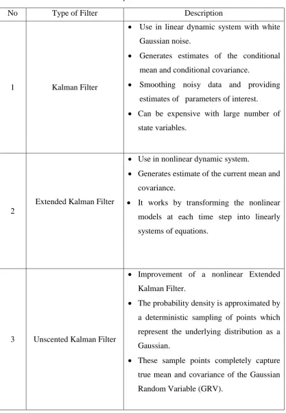
Table 2.1: Comparison of Gaussian Filter

No Type of Filter Description

1 Kalman Filter

 Use in linear dynamic system with white Gaussian noise.

 Generates estimates of the conditional mean and conditional covariance.

 Smoothing noisy data and providing estimates of parameters of interest.  Can be expensive with large number of

state variables.

2

Extended Kalman Filter

 Use in nonlinear dynamic system.

 Generates estimate of the current mean and covariance.

 It works by transforming the nonlinear models at each time step into linearly systems of equations.

3 Unscented Kalman Filter

 Improvement of a nonlinear Extended Kalman Filter.

 The probability density is approximated by a deterministic sampling of points which represent the underlying distribution as a Gaussian.

19

4 Cubature Kalman Filter

 Used for the nonlinear dynamic systems with additive process and measurement noise.

 Gaussian approximation of Bayesian Filter, but provides a more accurate filtering than existing Gaussian filters.

2.6 Technology Development

Based on previous studies, [17] can be used to propose a navigation algorithm that simultaneously locates the robots and updates landmarks in a manufacturing environment that can be used on mobile robots industry. In addition, the Kalman filter technique is used to construct the robot localisation problem [18]. Therefore, the techniques used to reduce the problem of robot locations and also contribute to technology development especially in the industry of mobile robots.

2.6.1 Landmark based Navigation of Industrial Mobile Robots

20

Figure 2.4: Landmarks and an on board laser scanner [17]

2.6.2 Robot Localisation and Kalman Filters

Rudy [18] did a project named Robot localisation and Kalman Filters. This project showed how to construct the robot localisation problem by using Kalman filter technique. Hence, the basic concepts involved in Kalman Filters and derive the equations of the basic filter that commonly used extensions. Other than that the types of filter that normally used were compared to show the difference between them. The disadvantage of this project is it is difficult to make the KF applicable in dynamic environments since the real world is not static. Figs. 2.5 and 2.6 show robot position and measurement model.

21

Figure 2.6: Measurement model [18]

2.6.3 Convergence and Consistency Analysis for Extended Kalman Filter Based SLAM

22

Figure 2.7: Robot movement [19]

2.6.4 LRF based Self Localization of Mobile Robot Using Extended Kalman Filter

A project called LRF based Self Localization of Mobile Robot using Extended Kalman Filter was designed by Songmin et. al. [20]. This paper presented a method of map building using interactive GUI for a mobile robot. The advantage of using this interactive GUI was the operator can modify map built by sensors, compared with the real time video from web camera. The disadvantage of this approach was there had several parts of errors for the line by using odometry data because of the surface roughness due to fails to get an accurately positioning. Fig. 2.8 shows robot movement.

23

2.6.5 Navigation of an autonomous mobile robot using EKF SLAM and Fast SLAM

[21] used EKF SLAM and Fast SLAM to introduce a probabilistic approach to a SLAM problem under Gaussian and non Gaussian conditions. They presented the navigation of an autonomous robot using Simultaneous Localization and Mapping (SLAM) in outdoor environments. Fast SLAM is an algorithm that used Rao-Blackwellised method for particle filtering, estimated the path of robot while the landmarks positions which were mutually independent and with no correlation, can be estimated by EKF. Hence, a real outdoor autonomous robot was presented and several experiments had been performed based on both methods. The disadvantages were no correlation between any pairs of landmarks in the map, while landmarks in this network were mutually independent. Figs. 2.9 and 2.10 show vehicle coordinate system and estimation of the trajectory using EKF with Gaussian implication.

24

Figure 2.10: Estimation of the trajectory using EKF with Gaussian Implication [21]

2.6.6 Mobile Robot Position Estimation Using Kalman Filter

Caius et. al [22] executed a project called Mobile Robot Position Estimation using Kalman Filter. This project presented the position estimation with the help of the Kalman Filter (KF) and the Extended Kalman Filter (EKF) for an autonomous mobile robot based on Ackermann steering. It focused on 2D model which was easier to implement while measurement by using overhead camera. The advantage of the proposed approach is two different method of filter that can be compared of the localisation accuracy between these two methods. The disadvantage of the approach is the position of robot is in unknown location that is difficult to know accurately the position of the robot. Figs. 2.11 and 2.12 show the trajectory estimation with the Kalman Filter and trajectory estimation with the Extended Kalman Filter.

77

REFERENCES

1. Rui, L., Maohai, L. & Lining, S. (2013). Image Features based Robot SLAM. Robotics and Biomimetics (ROBIO), IEEE International Conference, pp. 2499 – 2504.

2. Siegwart, R., Nourbakshsh & Scaramuzza, D. (2004). Introduction to Autonomous Mobile Robot. Journal ofIntelligent Robotic and Autonomous Agents, pp. 70-75.

3. Barrera, A. (2010). Mobile Robot Navigation. Journal of IEEE Transactions on Robotics and Automation, pp. 156-160.

4. Cheng, C. L. & Tummala, R. L. (1997). Mobile Robot Navigation using Artificial Landmarks. Journal of Robotic Systems, 14(2), pp. 93–106. 5. Sebastian, T., Wolfram B. & Dieter F. (2005). Probabilistic Robotic. The

MIT Press, pp. 365-387

6. Qingquan, L., Zhixiang, F. & Hanwu, Li. (2004). The Application of Integrated GPS and Dead Reckoning Positioning in Automotive Intelligent Navigation System. Journal of Global Positioning Systems, 3(1-2), pp. 183-190.

7. Parsley. (2006). Simultaneous Localisation and Mapping with Prior Information. Journalof Field Robotics, 31(3), pp. 212-235.

8. Zhang, W., Shoudong, H. & Gamini, D. (2007). Simultaneously Localization and Mapping. Journal ofIntelligent Robotic and Autonomous Agents, 3, pp. 1254- 1301.

78

10. Se, Lowe, S. & Little, D. (2001). Vision Based Mobile Robot Localization And Mapping Using Scale-Invariant Features. Robotics and Automation, 2001. Proceedings 2001 ICRA. IEEE International Conference on 2001,

2, 2051 – 2058.

11. Rao, An., H. W., Hu, Z. C., Mullane. & Joseph, A. (2013). Gaussian Particle Filter based Factorised Solution to the Simultaneous Localization and Mapping problem. Advanced Robotics and its Social Impacts (ARSO), IEEE Workshop, pp. 113 – 118.

12. Dick, S. (2009). Kalman filtering with state constraints A Survey of Linear and Nonlinear Algorithms. Published in IET Control Theory and

Applications, January 2009, pp. 1321-1342.

13. Abhishek, S. & Vishwanath, S. (2013). Localization of a Mobile Autonomous Robot using Extended Kalman Filter. Advances in Computing and

Communications Third International Conference, pp. 274 – 277.

14. Immanuel, A., Antonios, Peter, S. & Brian, W. (2004). Sensor Based Robot Localisation and Navigation using Interval Analysis and Extended Kalman Filter. 5th Asian Control Conference, pp. 2637-2643.

15. Liu, C. (2003). Unscented extended Kalman filter for target tracking Systems Engineering and Electronics. Journal of International Journal of Industry Robot, 22, pp. 188 – 192.

16. Jing, M., Yuan & Lee, C. (2011). Iterated Cubature Kalman Filter and its Application. Proceedings of the 2011, IEEE International Conference on Cyber Technology in Automation, Control, and Intelligent Systems, pp. 3212-3234.

17. Huosheng, H. & Dongbing, G. (2000). Landmark based Navigation of ` Industrial Mobile Robots. Emerging Technologies and Factory

Automation, 1999. Proceedings. ETFA 99. 1999 7th IEEE International

Conference, 1, pp. 121 – 128.

18. Rudy, N. (2003). Robot Localisation and Kalman Filters IEEE International Conference on 2000, pp. 1342-1365.

19. Shoundong, H. & Gamini, D. (2000). Convergence and Consistency Analysis for Extended Kalman Filter Based SLAM. Robotics IEEE Transactions,

79

20. Songmin, J., Yasuda, A., Chugo. & Takase, D. (2008). LRF based Self Localization of Mobile Robot Using Extended Kalman Filter. K. SICE Annual Conference, pp.2295 - 2298.

21. Sasiadek, J. Z., Monjazeb, A. & Necsulescu, D. (2004). Navigation of an Autonomous Mobile Robot using EKF SLAM and Fast SLAM. Control Conference, 2004. 5th Asian, IEEE International Symposium, pp. 72-77. 22. Caius, S., Cristina, Cruceru. & Florin. (1993).Mobile Robot Position

Estimation using Kalman Filter. Robotics and Automation, 1993. Proceedings., 1993 IEEE International Conference, pp. 373-379.

23. Pakki, K. B. C. , Gu, D.W. & Postlethwaith, I. (2010). SLAM using EKF, EH∞ and Mixed E / H∞ Filter. Intelligent Control (ISIC), IEEE International Symposium, pp. 3212-3243.

24. Pakki, K. B. C. , Gu, D.W. & Postlethwaith, I. (2011).Cubature Kalman Filter based Localization and Mapping. Robotics and Automation (ICRA), IEEE International Conference, pp. 3063-3068.

25. Gamini, D., Paul, N., Steven, C. & Huge, F. D. W. (2011). A Solution to the Simultaneous Localization and Map (SLAM) Problem. IEEE Transactions on Robotics and Automation,17(3), pp. 229-234.

26. Luigi, D. A., Andrea, G., Pietro, M. & Paolo, P. (2013). A Slam Algorithm for Indoor Mobile Robot Localisation Using an Extended Kalman Filter and a Segment Based Environment Mapping. Advanced Robotics (ICAR), 2013 16th International Conference, pp. 1920-1923.

27. Abhishek, S. & Vishwanath. (2013). Localisation of a Mobile Autonomous Robot using Extended Kalman Filter. Advances in Computing and

Communications (ICACC), 2013 Third International Conference, pp. 274 – 277.

28. Zhang, Q., Pei, H. & Zhang Cheng. (2014). A Mobile Robot Localisation and Map Building Algorithm and Simulation. Control Conference (CCC), 33rd Chinese 2014, pp. 3339 – 3344.

80