On Analysis and Evaluation of Comparative Performance for Selected Behavioral Neural Learning Models versus One Bio Inspired Non Neural Clever Model (Neural Networks Approach)

2016, Volume 3, e2933 ISSN Online: 2333-9721 ISSN Print: 2333-9705

On Analysis and Evaluation of Comparative

Performance for Selected Behavioral Neural

Learning Models versus One Bio-Inspired

Non-Neural Clever Model (Neural Networks

Approach)

Hassan M. H. Mustafa1, Fadhel Ben Tourkia1, Ramadan Mohamed Ramadan2

1_{Computer Engineering Department, Al-Baha Private College of Sciences, Al-Baha, KSA} 2_{Educational Psychology Department, Educational College, Banha University, Banha, Egypt}

Abstract

This piece of research addresses an interesting comparative analytical study, which considers two concepts of diverse algorithmic computational intelligent paradigms related tightly with Neural and Non-Neural Systems’ modeling. The first computa- tional paradigm was concerned with practically obtained psycho-learning behavioral results after three animals’ neural modeling. These are namely: Pavlov’s, and Thorn-dike’s experimental work. In addition, the third model is concerned with optimal solu-tion of reconstrucsolu-tion problem reached by a mouse’s movement inside Figure 8 maze. Conversely, second algorithmic intelligent paradigm was originated from observed activities’ results after Non-Neural bio-inspired clever modeling namely Ant Colony System (ACS). These results were obtained after attaining optimal solution while solving Traveling Sales-man Problem (TSP). Interestingly, the effect of increasing number of agents (either neurons or ants) on learning performance was shown to be similar for both introduced systems. Finally, performances of both intelligent learn-ing paradigms have been shown to be in agreement with learnlearn-ing convergence process searching for least mean square error LMS algorithm. While its application was for training some Artificial Neural Network (ANN) models. Accordingly, adopted ANN modeling is a relevant and realistic tool to investigate observations and analyze performance for both selected computational intelligence (biological behavioral learning) systems.

Subject Areas

Computer Engineering How to cite this paper: Mustafa, H.M.H.,

Tourkia, F.B. and Ramadan, R.M. (2016) On Analysis and Evaluation of Comparative Performance for Selected Behavioral Neural Learning Models versus One Bio-Inspired Non-Neural Clever Model (Neural Networks Approach). Open Access Library Journal, 3: e2933.

http://dx.doi.org/10.4236/oalib.1102933

Received: September 3, 2016 Accepted: October 28, 2016 Published: October 31, 2016

Copyright © 2016 by authors and Open Access Library Inc.

This work is licensed under the Creative Commons Attribution International License (CC BY 4.0).

Keywords

Artificial Neural Network Modeling, Animal Learning, Bio-Inspired Clever Algorithm, Ant Colony System, Traveling Salesman Problem

1. Introduction

This research work introduces a systematic investigational analysis for two naturally diversified adaptive learning phenomena’ paradigms. These diversified paradigms con-sider two typical behavioral learning performance algorithms of non-human creatures which were biologically classified as Neural (animals), and Non-Neural (ant colonies) Systems’ modeling [1]-[6].

The first paradigm is associated to adaptive neural behavioral learning inside three animals’ brain: a Dog, a Cat, and a Mouse. However, the second belongs to analysis of bio-inspired behavioral learning associated to ant colony optimization for observed swarm intelligence phenomenon aiming to get optimal solution Traveling Salesman Problem (TSP), based on realistic simulation foraging of behavioral phenomenon ob-served by real Ant Colony System. Analysis and evaluation of such interdisciplinary challenging learning issue are carried out using Neural Networks’ Conceptual Ap-proach. Herein, this paper presents analytical details for both intelligent behavioral ap-proaches, which were considered via two hand folds as follows. Firstly, on one hand: autonomous inferences and perceptions were performed in nature by non-human brain (animals: Dogs, Cats, and Mice). Secondly, on the other hand paradigm is inspired by source of ant colony optimization originated from intelligent foraging behavioral phe-nomenon observed by real ant colonies in natural environment. This behavior is ex-ploited in artificial ant colonies for the search of approximate solutions to optimization problems namely Traveling Salesman Problem (TSP).

1.1. First Learning Paradigm

More specifically, the first behavioral algorithmic paradigm considers three nonhuman models. All three neural creatures’ models have been inspired by results observed after behavioral psycho-learning performance in natural real world. Two of introduced models are based on Pavlov’s and Thorndike’s excremental work. In some details, Pav-lov’s dog learns how to associate between two inputs sensory stimuli (audible, and visu-al signvisu-als). However, Thorndike’s cat behaviorvisu-al learning tries to get out from a cage to reach food out of the cage. Both behavioral learning models improve their performance by trial to minimize response time period. The third model is concerned with behavior-al learning of mouse while performing tribehavior-als for getting out from inside Figure 8 maze. That is performed as optimal trial to solve reconstruction problem [7].

1.2. Second Learning Paradigm

TSP by using non-neural systems namely, colony system ACS. That model simulates a swarm (ant) intelligent system used for solving TSP optimally. Briefly, ACS algorithm is inspired by the foraging behavior of ants, specifically the pheromone communication between ants regarding a good path between the colony and a food source in an envi-ronment. This mechanism is called stigmergy. Interestingly, that mechanism performed by bringing food from different food sources to store (in cycles) at ant’s nest. Interes-tingly, all of presented models herein shown to behave analogously in agreement with Least Mean Square LMS Algorithm previously suggested at ANN learning.

Principles of biological information processing concerned with learning convergence for both bio-systems have been published at [8][9][10]. By some details, in this work an interesting comparative analysis introduced for concepts of behavioral learning phenomenon, versus optimal solution of TSP using swarm intelligence optimization (ACS) [1][10][11][12]. In other words, an investigational analytical overview is pre-sented herein to get insight with behavioral intelligence of non-human creatures’ per-formance as Neural and Non-Neural Systems [1][4][5][12].

Briefly, analysis of obtained results by such recent research work leads to discovery of some interesting analogous relations between both behavioral learning paradigms. That concerned with observed resulting errors, time responses, learning rate values, gain factor values versus number of trials, training dataset vectors intercommunication among ants and number of neurons as basic processing elements [5][13][14]. Howev-er, it seems to observe diversity of behavioral learning curves performance (till reaching optimum state) for proposed biological systems, both are similar to each other (consi-dering normalization of performance curves) [3] [6]. Interestingly, behavioral intelli-gence & learning performance phenomena carried out by both nonhuman biological systems are characterized by their adaptive behavioral responses to their living envi-ronmental conditions. So, all introduced models for both approaches consider input stimulating actions provided by external environmental conditions versus adaptive reactions carried by creatures’ models [1][9][15].

The rest of this paper is organized as follows. At next section, a simple interactive learning model is presented along with a generalized ANN block diagram simulating learning process. Revising of Thorndike’s, Pavlov’s, and mouse’s behavioral learning are introduced briefly at the third section. The fourth section is dedicated to illustrate learning algorithm at ACS.

Obtained simulation results compared with the experimental results are given at the fifth section. Finally, at the last sixth section, some conclusions and valuable discussions are introduced.

2. Interactive Learning Model

2.1. Simplified Interactive Learning Process

How-ever, correction signal(s) in the case of learning with a teacher given by output re-sponse(s) of the model that evaluated by either the environmental conditions (unsu-pervised learning) or by supervision of a teacher. Furthermore, the teacher plays a role in improving the input data (stimulating learning pattern) by reducing the noise and redundancy of model pattern input. That is in accordance with tutor’s experience while performing either conventional (classical) learning or CAL. Consequently, he provides the model with clear data by maximizing its signal to noise ratio [12]. Conversely, in the case of unsupervised/self-organized learning, which is based upon Hebbian rule [15], it is mathematically formulated by Equation (7). For more details about mathe-matical formulation describing a memory association between auditory and visual sig-nals, please refer to [16].

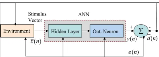
The presented model given in Figure 2 generally simulates two diverse learning pa-radigms. It presents realistically both paradigms: by interactive learning/ teaching process, as well as other self-organized (autonomous) learning. By some details, firstly is concerned with classical (supervised by a tutor) learning observed in our classrooms (face to face tutoring). Accordingly, this paradigm proceeds interactively via bidirec-tional communication process between a teacher and his learners (supervised learning) [16][17]. However, the second other learning paradigm performs self-organized (au-tonomously unsupervised) tutoring process [16].

2.2. Mathematical Formulation of Learning Paradigms

Referring to above Figure 2; the error vector e n

( )

during learning processes is given by:

Figure 1. Simplified view for interactive learning process.

( )

( )

( )

e n =y n −d n (1)

where e n

( )

process, y n

( )

( )

Moreover, the following four equations are deduced:

( )

( ) ( )

k j kj

V n =X n W n (2)

( )

(

( )

)

(

)

(

)

k k

Y n =ϕ V n = − −λ + −λ (3)

( )

( )

( )

k k k

e n = d n −y n (4)

(

)

( )

( )

kj kj kj

W n+ =W n + ∆W n (5)

where X is input vector and W is the weight vector. φ is the activation function. Y is the output. ek is the error value and dk is the desired output. Note that ∆Wkj

( )

dynamical change of weight vector value. Above four equations are commonly applied for both learning paradigms: supervised (interactive learning with a tutor), and unsu-pervised (learning though student’s self-study). The dynamical changes of weight vec-tor value specifically for supervised phase is given by:

( )

( ) ( )

kj k j

W n ηe n X n

∆ = (6)

where η is the learning rate value during the learning process for both learning para-digms. At this case of supervised learning, instructor shapes child’s behavior by posi-tive/negative reinforcement Also, Teacher presents the information and then students demonstrate that they understand the material. At the end of this learning paradigm, assessment of students’ achievement is obtained primarily through testing results. However, for unsupervised paradigm, dynamical change of weight vector value is given by:

( )

( ) ( )

kj k j

W n ηY n X n

∆ = ₍₇₎

Noting that ek

( )

( )

in-stant (n) during the learning process. Instructor designs the learning environment.

3. Models of First Learning Paradigm

3.1. Revising of Pavlov’s Work [11]

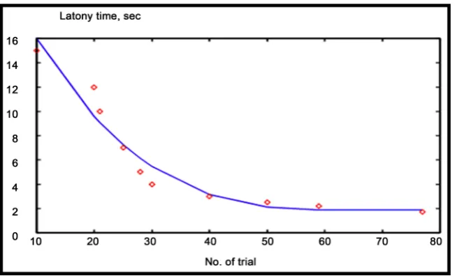
sponta-neously developed in a form of some number of salivation drops representing response signals intensities. These intensities observed to be in proportionality with the increase of the subsequent number of trials. So, this relation agrees with odd sigmoid function curve as reaching saturation state [3][4]. Conversely, on the basis of Pavlov’s obtained experimental results, it is well observed mathematical interrelationship between latency time period versus subsequent number of trials can be illustrated explicitly in the form of hyperbolic function curve that mathematically expressed by following equation:

( )

t n nβ

α

= ₍₈₎

where α and β are arbitrary positive constant in the fulfillment of some curve fitting to a set of points as shown by graphical relation illustrated in Figure 3.

3.2. Revising of Thorndike’s Work [12]

Referring to behaviorism learning theory presented at [19], Thorndike had suggested three principles, which instructors (who adopted teaching based on behaviorism learn-ing theory) should apply in order to promote effectiveness of behavioral learnlearn-ing process. These principles are given as follows:

• _{Present the information to be learned in small behaviorally defined steps.}

• _{Give rapid feedback to pupils regarding the accuracy of their learning. (Learning} being indicated by overt pupil responses).

• _{Allow pupils to learn at their own pace.}

Furthermore, building on these he proposed an alternative teaching technique called programmed learning/instruction and also a teaching machine that could present pro-grammed material. Initially, cat’s performance trials results in random outputs. By se-quential trials, following errors observed to become minimized, by increasing number of training (learning) cycles. Referring to Figure 4, which illustrates original Thorn-dike’s work results. This figure presents the relation between response time and num-

Figure 4. The original result of Thorndike representing learning performance for a cat to get out from the cage for reaching food.

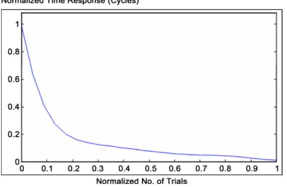
Figure 5. Thorndike normalized results seem to be closely similar to exponential time decay.

ber of trials. Furthermore, referring to that original Thorndike’s experimental results given at Figure 4, represent behavioral learning performance of Thorndike’s work. However, normalized learning curve that presents performance curve of experimental work is given approximately at Figure 5. Interestingly, the comparative analogy be-tween performance curves of Pavlov’s and Thorndike’s work shown to behave similar to each other [4].

Referring to Figure 6, it observed that by increasing number of training cycles, the first learning algorithm converges to some fixed limiting values (for normalized time response). That observed results consider normalization of both number of trials values versus their corresponding normalized time response (for both original experimental work of Pavlov and Thorndike given at Figure 3 & Figure 4 respectively).

3.3. Mouse’s Trails for Solving Reconstruction Problem

Referring to [18], the timing of spikes in a population of neurons can be used to recon-struct a physical variable is the reconrecon-struction of the location of a rat in its environment from the place fields of neurons in the hippocampus of the rat. In the experiment re-ported here, the firing part-terns of 25 cells were simultaneously recorded from a freely moving mouse [7]. The place cells were silent most of the time, and they fired max-imally only when the animal’s head was within restricted region in the environment called its place field [19]. The reconstruction problem was to determine the rat’s posi-tion based on the spike firing times of the place cells. Bayesian reconstrucposi-tion was used to estimate the position of the mouse in the Figure 8 maze shown at Figure 7, which adapted from [6]. Assume that a population of N neurons encodes several variables

(

)

(

)

n= n n  n fired by the N neurons within a time interval τ , we want to esti-mate the value of x using the Bayes rule for conditional probability:

(

)

(

) ( ) ( )

P x n =P n x P x P n (9)

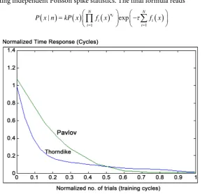
Assuming independent Poisson spike statistics. The final formula reads

(

)

( )

( )

( )

1 1

| i exp

N N

n

i i

i i

P x n kP x f x τ f x

= =

   

= _{  }− _

 



∏

∑

where k is a normalization constant, P(x) is the prior probability, and fi(x) is the meas-ured tuning function, i.e. the average firing rate of neuron i for each variable value x. The most probable value of x can thus be obtained by finding the x that maximizes

(

)

P x n , namely,

(

)

ˆ arg max |

x= P x n (11)

By sliding the time window forward, the entire time course of x can be reconstructed from the time varying-activity of the neural population. This appendix illustrates well Referring to results for solving reconstruction (pattern recognition) problem solved by a mouse in Figure 8 maze [7] [21]. That measured results based on pulsed neuron spikes at hippocampus of the mouse brain. In order to support obtained investigational research results and lightening the function of mouse’s brain hippocampus area, three findings have been announced recently as follows:

1) Referring to [22], experimental testing performed for hippocampal brain area ob-served neural activity results in very interesting findings. Therein, ensemble record-ings of 73 to 148 rat hippocampal neurons were used to predict accurately the ani-mals’ movement through their environment, which confirms that the hippocampus transmits an ensemble code for location. In a novel space, the ensemble code was initially less robust but improved rapidly with exploration. During this period, the activity of many inhibitory cells was suppressed, which suggests that new spatial in-formation creates conditions in the hippocampal circuitry that are conducive to the synaptic modification presumed to be involved in learning. Development of a new population code for a novel environment did not substantially alter the code for a familiar one, which suggests that the interference between the two spatial represen-tations was very small. The parallel recording methods outlined here make possible the study of the dynamics of neuronal interactions during unique behavioral events. 2) The hippocampus is said to be involved in “navigation” and “memory” as if these

were distinct functions [23]. In this issue of Neuron this research paper evidence has been provided that the hippocampus retrieves spatial sequences in support of mem-ory, strengthening a convergence between the two perspectives on hippocampal function.

distance in a situation where these dimensions neuronal networks captured both the organization of time and distance in a situation where these dimensions dominated an ongoing experience as illustrated at Figure 7[24].

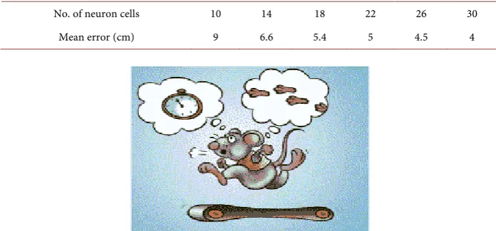
According to following Table 1, the error value seems to decrease similar to expo-nential curve decays to some limit value versus (place field) cells.

Noting that, the value of mean error converges (by increase of number of cells) to some limit, excluded as Cramer-Rao bound. That limiting bound is based on Fisher’s information given as tabulated results in the above and derived from [21]. That implies LMS algorithm is valid and obeys the curve.

Furthermore, it is noticed that the algorithmic performance learning curve referred to Figure 7, converged to bounding limit (of minimum error value) fixed Cramer Rao bound (Limiting value). That is analogous to minimum time response corresponding to maximum number of trials limit by referring to above Figure 2. Interestingly, consi-dering comparison between learning curve performances at Figure 8 and learning that at ACS. It observed the analogy when comparing number of place field cells (at hippo-campus mouse’s brain area) versus the number of cooperative ants while searching for optimized TSP solution adopting ACS. More details are presented at the simulation re-sults’ Section 5.

4. Second Learning PARADIGM

4.1. Revising Ant Colony System Performance

Referring to Figure 1, ants are moving on a straight line that connects a food source to their nest. It is well known that the primary means for ants to form and maintain the line is a pheromone trail. Ants deposit a certain amount of pheromone while walking, and each ant probabilistically prefers to follow a direction rich in pheromone. This elementary behaviour of real ants can be used to explain how they can find the shortest

Table 1. Relation between number of cells and mean error in solving reconstruction problem.

No. of neuron cells 10 14 18 22 26 30

Mean error (cm) 9 6.6 5.4 5 4.5 4

Figure 8. The dashed line indicates the approach to Cramer-Rao bound based on Fisher infor-mation adapted from [6].

path that reconnects a broken line after the sudden appearance of an unexpected ob-stacle has interrupted the initial path (Figure 9(A)). In fact, once the obstacle has ap-peared, those ants which are just in front of the obstacle cannot continue to follow the pheromone trail and therefore they have to choose between turning right or left. In this situation we can expect half the ants to choose to turn right and the other half to turn left (Figure 9(B)). A very similar situation can be found on the other side of the ob-stacle (Figure 9(C)). It is interesting to note that those ants which choose, by chance, the shorter path around the obstacle will more rapidly reconstitute the interrupted pheromone trail compared to those which choose the longer path. Thus, the shorter path will receive a greater amount of pheromone per time unit and in turn a larger number of ants will choose the shorter path. Due to this positive feedback (autocatalyt-ic) process, all the ants will rapidly choose the shorter path (Figure 9(D)). The most interesting aspect of this autocatalytic process is that finding the shortest path around the obstacle seems to be an emergent property of the interaction between the obstacle shape and ants distributed behaviour: although all ants move at approximately the same speed and deposit a pheromone trail at approximately the same rate, it is a fact that it takes longer to contour obstacles on their longer side than on their shorter side which makes the pheromone trail accumulate quicker on the shorter side. It is the ants’ prefe-rence for higher pheromone trail levels which makes this accumulation still quicker on the shorter path. This process is adapted with the existence of an obstacle through the pathway from nest to source and vice versa, however, more detailed illustrations are given through other published research work, [1]. Therein, ACS performance obeys computational biology algorithm used for solving optimally travelling salesman prob-lem TSP [1].

typically applied to search and optimization domains. That simulation the foraging be-havioral intelligence of a swarm (ant) system used for reaching optimal solution of TSP a cooperative learning approach to the traveling salesman problem optimal solution of TSP considered using realistic simulation of bio-inspired clever Non-neural model namely: ACS [27].

Referring to two more recent research work [2][24], an interesting view distributed biological system ACS is presented. Therein, the ant Temnothorax albipennis uses a learning paradigm (technique) known as tandem running to lead another ant from the nest to food with signals between the two ants controlling both the speed and course of the run. That learning paradigm involves bidirectional feedback between teacher and pupil and considered as supervised learning [24][25][26][28].

ACS optimization process versus MICE reconstruction problem. Finally the relation between cooperative process in ACS and activity at hippocampus of the mouse brain is illustrated well at two recently published works [3][4].

4.2. Cooperative Learning by ACS for Solving TSP

Cooperative learning by Ant Colony System for solving TSP referring to Figure 9, which adapted from [1], the difference between communication levels among agents (ants) develops different outputs average speed to optimum solution. The changes of communication level are analogues to different values of λ in sigmoid function as shown at Equation (13) in below. This analogy seems to be illustrated well as referring to Figure 4 where the output salivation signal is increased depending upon the value of no of training cycles. When the number of training cycles increases virtually to an infi-nite value, the number of salivation drops obviously reach a saturation value addition-ally the pairing stimulus develops the learning process turned in accordance with Heb-bian learning rule [17]. However in case of different values of λ other than zero impli-citly means that output signal is developed by neuron motors.

5. Simulation Results

5.1. Intercommunication among Ants

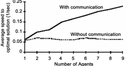
Referring to Figure 10 shown in below, the relation between tour lengths versus the CPU time is given. It is observed the effect of ant cooperation level on reaching opti-mum (miniopti-mum tour). Obviously, as level of cooperation among ants increases (better communication among ants) the CPU time needed to reach optimum solution is de-creased. So, that optimum solution is observed to be reached (with cooperation) after 300 (msec) CPU the while that solution is reached after 600 (msec) CPU time (without cooperation).

In other words, by different levels of cooperation (communication among ants) the optimum solution is reached after CPU time τ placed somewhere between above two limits 300 - 650 (M. sec). Referring to [1], cooperation among processing agents (ants) is a critical factor affecting ACS performance as illustrated at Figure 11. So, the number of ants required to get optimum solution differs in accord with cooperation levels among ants. This number is analogous to number of trials in OCR process. Interesting-

Figure 10. Illustrates performance of ACS with and without communication between ants,

adapted from [1].

ly, in natural learning environment, the (S/N) signal to noise ratio is observed to be di-rectly proportional to leaning rate parameter in self-organized ANN models. That means in less noisy learning environment (clearer) results in better outcome learning performance given in more details at [19][29]. More precisely, such learning environ-ment with better (S/N) ratio, implicitly results in increasing of stored experience (inside synaptic connectivity) while nonhuman creatures are adopting self-organized learning via interaction with environment [17]. Referring to Equation (11) introduced for solv-ing reconstruction problem (correspondsolv-ing to the most probable value of x) has great similarity to the equation presented to search for optimal solution considering TSP reached by ACS (for random variable S) as follows.

( )

( )

{

}

arg max , , if

otherwise k

u M r u r u q q

s S β τ η ∈  _{  ⋅  ≤}      = 

 (12)

where τ(r,u) is the amount of pheromone trail on edge (r,u), η(r,u) is a heuristic func-tion, which was chosen to be the inverse of the distance between cities r and u, β is a parameter which weighs the relative importance of pheromone trail and of closeness, q is value chosen randomly with uniform probability in [0, 1], q0 (0 ≤ q0 ≤ 1) is a para-meter, Mk is memory storage for k ants activities, and S is a random variable selected according to some probability distribution [24] [25]. Synergistic effect by Ant colony intercommunications is given by mathematical formulation for ACS optimization as follows. At recent previous work analogy between ACS performance and ANNs has been illustrated at [2][5][6][30][31][32]. The performance of the synergistic effect of ACS referring to the generalized sigmoid function is given as function of discrete in-teger (+ve) value representing for number of ants as follows:

( )

1 e n n f n λ λ

α − −₋ 

=  ₊ 

  (13)

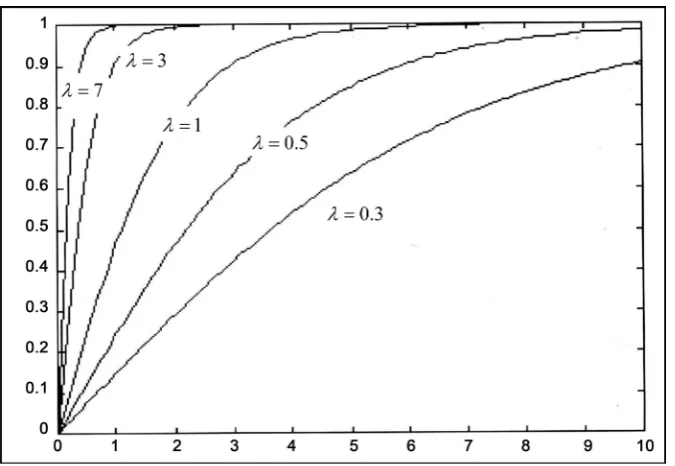
where α … is an amplification factors representing asymptotic value for maximum av-erage speed to get optimized solutions and λ in the gain factor changing in accords with communication between ants. However by this mathematical formulation of that mod-el normalized behavior it is shown that by changing of communication levmod-els (represented by λ) that causes changing of the speeds for reaching optimum solutions. More appropriate that declares the slope (gain factor) for suggested sigmoid function is a direct measure for intercommunications level among ants in ACS in other words, the slope, λ is directly proportional to pheromone trail mediated communication among agents of ACS. Consequently, ACS global performance has become nearly parallel (slope = 0) to the X-axis (number of ants), nevertheless increasing of ants comprising tested colony (slope, λ = 0), that’s the case when no intercommunications between ants exists.

In the given Figure 12, it is illustrated that normalized model behavior according to following equation.

( )

(

(

(

)

)

)

(

(

(

)

)

)

Figure 12. Graphical representation of learning performance of ACS model with different com-munication levels (λ).

where λi represents one of gain factors (slopes) for sigmoid function.

5.2. Realistic Simulation Program

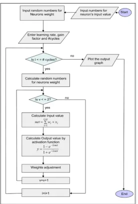
By referring to Figure 13, it introduces the flowchart for simulation program which applied for performance evaluation of behavioral learning processes. Considering the two adopted cases of biological creatures having either neural or non-neural systems. That figure presents a simplified macro-level flowchart which describes briefly algo-rithmic steps for realistic simulation program of adopted Artificial Neural Networks’ model for different number of neurons using. The results are shown at the three Fig-ures 14-16 after that program running.

5.3. Least Mean Square LMS Algorithm

At the Figure 14, it presents the learning convergence process for least mean square error as used for training of ANN models [18]. It is clear that this process performed similarly as ACS searching for minimum tour when solving TSP [1]. Furthermore, it obeys the learning performance observed during psycho experimental work carried for animal learning [3].

6. Conclusions and Discussion

According to the above animal learning experiments (dogs, cats, and mice), and their analysis and evaluation by ANNs_{modeling, all of them agree well as for ACS,}

Figure 13. A simplified macro level flowchart describing algorithmic steps for Artificial Neural Networks modeling considering various neurons’ number.

Figure 15. Illustrate learning performance error-rate with different gain factors when #cycles = 300 and Learning rate = 0.3.

Figure 16. Illustrate learning performance error-rate with different learning rates when #cycles = 300 and gain factor = 1.

Pavlov are commonly characterized by their hyperbolic decay and also, both obey ge-neralized LMS for error minimization by learning convergence.

In this context, the algorithm agrees with the behavior of brainier mouse behavior (that is genetically reformed) as illustrated at [16]. Generally, the four introduced non-human models in this work perform their behavioral learning functions similar to LMS error algorithm, which is introduced at Figure 17.

Figure 17. Idealized learning curve of the LMS algorithm adapted from [18].

algorithms for the presented four models are close to each other with similar iterative steps (either explicitly or implicitly). Finally, it is worthy to note that the rate of in-crease of salivation drops is analogous to rate for reaching optimum average speed in ACS optimization process. Similarly, this rate is also analogous to speed of cat getting out from cage in Thorndale’s experiment. It is noted that, increase on number of artifi-cial ants is analogous to number of trials in Pavlov’s work.

References

[1] Dorigo, M. and Stutzle, T. (2004) Ant Colony Optimization. MIT Press, Boston.

[2] Hassan, H.M. (2011) On Mathematical Modeling of Cooperative E-Learning Performance during Face to Face Tutoring Sessions (Ant Colony System Approach). IEEE Conference on Education Engineering-Learning Environments and Ecosystems in Engineering Educa-tion, Amman, 4-6 April 2011, 338-346.

[3] Hassan, H. and Watany, M. (2000) On Mathematical Analysis of Pavlovian Conditioning Learning Process Using Artificial Neural Network Model. 10th Mediterranean Electro Technical Conference, Cyprus, 29-31 May 2000.

[4] Hassan, H.M. and Watany, M. (2003) On Comparative Evaluation and Analogy for Pavlo-vian and Throndikian Psycho-Learning Experimental Processes Using Bioinformatics Modeling. AUEJ, 6, 424-432.

[5] Hassan, H.M. and Al-Hamadi, A. (2009) On Comparative Analogy between Ant Colony Systems and Neural Networks Considering Behavioral Learning Performance. 4th Indian International Conference on Artificial Intelligence (IICAI), Tumkur, 16-18 December 2009. [6] Mustafa, H.M.H., et al. (2013) Comparative Analogy of Neural Network Modeling versus

Ant Colony System (Algorithmic and Mathematical Approach). Proceeding of Internation-al Conference on DigitInternation-al Information Processing, E-Business and Cloud Computing

(DIPECC), Dubai, 23-25 October 2013.

http://sdiwc.net/conferences/2013/dipecc2013/

[7] Zhang, K., et al. (1998) Interpreting Neuronal Population Activity by Reconstruction.

Journal of Neurophysiology, 79, 1017-1044.

Conference on Computational Intelligence for Modelling, Control and Automation, Vien-na, 28-30 November 2005, 647-653.http://dx.doi.org/10.1109/cimca.2005.1631542

[9] Brownlee, J. Clever Algorithms: Nature-Inspired Programming Recipes.

http://www.cleveralgorithms.com/nature-inspired/swarm/ant_colony_system.html

[10] Hassan, H.M. (2005) On Learning Performance Evaluation for Some Psycho-Learning Ex-perimental Work versus an Optimal Swarm Intelligent System. International Symposium on Signal Processing and Information Technology, Athens, 18-20 December 2005.

[11] Pavlov, I.P. (1927) Conditional Reflex: An Investigation of the Psychological Activity of the Cerebral Cortex. Oxford University Press, New York.

[12] Thorndike, E.L. (1911) Animal Intelligence. Ct. Hafner, Darien.

[13] Hampson, S.E. (1990) Connectionistic Problem Solving. Computational Aspects of Biolog-ical Learning. Birkhouser, Berlin.http://dx.doi.org/10.1007/978-1-4684-6770-3

[14] Ghonaimy, M.A., Al-Bassiouni, A.M. and Hassan, H.M. (1994) Leaning of Neural Networks Using Noisy Data. 2nd International Conference on Artificial Intelligence Applications, Cairo, 22-24 January 1994, 387-399.

[15] Jilk, D.J., Cer, D.M. and O’Rilly, R.C. (2003) Effectiveness of Neural Network Learning Rules Generated by a Biophysical Model of Synaptic Plasticity. Technical Report, Depart-ment of Psychology, University of Colorado, Boulder.

[16] Hebb, D.O. (1949) The Organization of Behaviour. Wiley, New York.

[17] Fukaya, M., et al. (1988) Two Level Neural Networks: Learning by Interaction with Envi-ronment. 1st International Conference on Neural Networks, San Diego, 24-27 July 1988. [18] Haykin, S. (1999) Neural Networks. Prentice-Hall, Englewood Cliffs, 50-60.

[19] Hassan, H.M. (2005) On Mathematical Analysis, and Evaluation of Phonics Method for Teaching of Reading Using Artificial Neural Network Models. International Conference on

Management of Data and Symposium on Principles Database and Systems, Baltimore,

17-19 January 2005, 254-262.

[20] Hassan, M.H. (2008) A Comparative Analogy of Quantified Learning Creativity in Humans versus Behavioral Learning Performance in Animals: Cats, Dogs, Ants, and Rats. A Con-ceptual Overview. Workshop and Summer School on Evolutionary Computing, Derry, 18-22 August 2008.

[21] Keesee, G. Learning Theories.

http://teachinglearningresources.pbworks.com/w/page/19919565/Learning%20Theories

[22] Wilson, M.A. and McNaughton, B.L. (1993) Dynamics of the Hippocampal Ensemble Code for Space. Science, 261, 1055-1058. http://www.ncbi.nlm.nih.gov/pubmed/8351520

http://dx.doi.org/10.1126/science.8351520

[23] Eichenbaum, H. (2013) Hippocampus: Remembering the Choices. Neuron, 77, 999-1001.

http://www.researchgate.net/publication/236073863_Hippocampus_remembering_the_cho ices

http://dx.doi.org/10.1016/j.neuron.2013.02.034

[24] Kraus, B.J., Robinson, R.J., White, J.A., Eichenbaum, H. and Hasselmo, M.E. (2013) Hip-pocampal “Time Cells”: Time versus Path Integration. Neuron, 78, 1090-1101.

http://www.ncbi.nlm.nih.gov/pubmed/23707613

http://dx.doi.org/10.1016/j.neuron.2013.04.015

[25] Bonabeau, E. and Theraulaz, G. (2001) Swarm Smarts. Majallat Aloloom, 17, 4-12. [26] Bonabeau, E., Dorigo, M. and Theraulaz, G. (1999) Swarm Intelligence: from Natural to

[27] Kennedy, J., Kennedy, J.F., Eberhart, R.C. and Shi, Y. (2001) Swarm Intelligence (The Mor-gan Kaufmann Series in Evolutionary Computation). MorMor-gan Kaufmann, Burlington, 81-86.

[28] Rechardson, T. and Franks, N.R. (2006) Teaching in Tandem-Running Ants. Nature, 439,

153.http://dx.doi.org/10.1038/439153a

[29] Hassan, M.H. (2005) On Quantitative Mathematical Evaluation of Long Term Potentiation and Depression Phenomena, Using Neural Network Modeling. International Conference on Simulation and Modeling, Bangkok, 17-19 January 2005, 237-241.

[30] Alberto, C., et al. (1991) Distributed Optimization by Ant Colonies. Elsevier, Amsterdam, 134-142.

[31] Hassan, H.M. (2005) On Learning Performance Evaluation for Some Psycho-Learning Ex-perimental Work versus an Optimal Swarm Intelligent System. International Symposium on Signal Processing and Information Technology, Athens, 18-20 December 2005.

[32] Hassan, H.M. (2008) On Comparison between Swarm Intelligence Optimization and Beha-vioral Learning Concepts Using Artificial Neural Networks (An Overview). 14th Interna-tional Conference on Information Systems Analysis and Synthesis (ISAS), Orlando, 29 June-2 July 2008.

Submit or recommend next manuscript to OALib Journal and we will provide best service for you:

 _{Publication frequency: Monthly}

 _{9 subject areas of science, technology and medicine}

 Fair and rigorous peer-review system

 _{Fast publication process}

 Article promotion in various social networking sites (LinkedIn, Facebook, Twitter, etc.)

 _{Maximum dissemination of your research work}