Constrained Feedback Stabilization for Bilinear Parabolic Systems

(1)

http://dx.doi.org/10.4236/ica.2015.62011

Constrained Feedback Stabilization for

Bilinear Parabolic Systems

Azzeddine Tsouli, Ali Boutoulout

TSI Team, MACS Laboratory, Faculty of Sciences, Moulay Ismail University, Meknes, Morocco Email: [email protected], [email protected], [email protected]

Received 2 January 2015; accepted 27 March 2015; published 30 March 2015

This work is licensed under the Creative Commons Attribution International License (CC BY).

http://creativecommons.org/licenses/by/4.0/

Abstract

In this paper, we shall study the stabilization and the robustness of a constrained feedback control for bilinear parabolic systems defined on a Hilbert state space. Then, we shall show that stabiliz-ing such a system reduces stabilization only in its projection on a suitable subspace. For this pur-pose, a new constrained stabilizing feedback control that allows a polynomial decay estimate of the stabilized state is given. Also, the robustness of the considered control is discussed. An illu-strating example and simulations are presented.

Keywords

Bilinear Parabolic Systems, Constrained Feedback Stabilisation, Decay Estimate, Robustness

1. Introduction

(2)

this paper, we are concerned with the question of the stabilization by a constrained feedback control for bilinear parabolic systems that can be described in the following form:

( )

_{( )}

_{( ) ( )}

_{( )}

0

, 0 d

d

y

Ay p B y t

t t y t y

t = + = (1)

on a real Hilbert space H with inner product .,. ; and corresponding norm . , where the linear operator A

generates a contraction semigroup

(

( )

)

0

t

S t _≥ on H and B∈

( )

H . While the real valued function

( )

2

(

)

. 0, ;

p ∈L +∞  represents a control. A function y

( )

. ∈

(

0, ;t H0

)

, t0 >0, is a mild solution of the

sys-tem (1) if and only if the solution y t

( )

of the system (1) satisfies the variation of parameters formula:

( )

0 ₀

(

) ( ) ( )

d , 0

t

y t =S t y +

∫

S t−τ p τ By τ τ t≥ (2)

(see [3]). By choosing an adequate feedback control p t

( )

in such a way, the corresponding solution y t

( )

of the system (1) converges to zero when t→ +∞, for all y0 in H . For finite-dimensional bilinear systems

as-sociated to a skew-adjoint matrix A, the question of stabilization has been treated in [4], under the condition:

(

)

(

)

(

)

{

0 1

}

{ }

span Az ad, A B z ad, , A B z, ,,adk A B z, , =n, ∀ ∈z n− 0 (3) where adk

(

A B,

)

is defined recursively as ad0

(

A B,

)

=B, ad1

(

A B,

)

=AB−BA and

(

)

(

)

1 1

, , ,

k k

ad + A B =ad A ad A B , ∀ ∈k . Using the following assumptions:

( )

exp , exp 0,, 0 0

B tA y tA y = ∀ ≥ ⇒ =t y (4) the problem of stabilization has been studied in [5]. In [3], when the linear operator B is compact and

( )

(

S t

)

_t_≥₀ is a contraction semigroup, then using the quadratic feedback control

( )

0 ,

p t = − y t By t (5) a weak stabilization result is obtained under the weak observability condition:

( )

t ,

( )

0, 0 0

BS y S t y = ∀ ≥ ⇒ =t y (6) In the case where B is sequentially continuous from Hw (H endowed with the weak topology) to H, the quadratic feedback control (2) weakly stabilizes the system (1), provided that the following weak observabil-ity assumption (4) holds (see [3]). Under the exact observability assumption

( )

2

(

)

0 , d , , , 0

T

BS t y S t y t≥δ y ∀ ∈y H T δ >

∫

(7)

The strong stabilization result with the following decay estimate

( )

t 1 , as

y t

t

 

= _ _ → +∞

 

 (8)

i.e. y t

( )

M t

≤ , M >0 for t large enough, has been obtained using the quadratic feedback control (5) (see [6]). However, in this way the convergence of the resulting closed loop state is not better than (8). In [7] the ra-tional decay rates are established i.e. using the following feedback control:

( )

(

)

,

, 2

r r

t t t

t y By

p r

y

(3)

It has been shown in [8] that, where the resolvent of the operator A is compact, and B is abounded linear, self-adjoint and monotone, the constrained feedback control law

( )

( ) ( )

,

1 ,

t t

By y

p

B t

t y t y = −

+ (9)

strongly stabilizes the system (1), provided that the assumption (6) holds. It has been established in [7] that, if the linear operator A generates a contraction semigroup

(

( )

)

0

t

S t _≥ in H, then the system (1) is strongly stable with the explicit decay estimate (8), using the control (9), provided that the estimate (7) holds. Here, we will establish an explicit decay estimate of the stabilized state and the robustness of the control (9) for a large class of bilinear systems as considered in [3] [8] [9]. The method used in this paper is based on decomposing the system (1) into two suitable subsystems: the stable part and the unstable one. Then, we will show that one can concentrate on the determination of a stabilizing control for the so-called unstable part which maintains the ex-ponential stability of the stable part. The rest of this article is as follows: in Section 2, we will give the main potheses that allow the decomposition of the system (1) into two subsystems. Then, under the compactness hy-pothesis of the operator B, we will give a weaker variant of the condition (6) which achieves strong stabiliza-tion of the system (1). In Secstabiliza-tion 3, we will show that under a weaker version of (6), we obtain the stabilizastabiliza-tion with the decay estimate (8). Section 4 concerns the robustness of the stabilizing controls. The last section is de-voted to an illustrating example and simulations.

2. Stabilization Results

Let us now recall the following definition concerning the asymptotic behavior of the system (1).

2.1. Definition

The system (1) is weakly (resp. strongly) stabilizable if there exists a feedback control p t

( )

= f y

(

( )

t

)

, t≥0

: :

f H→K =,  such that the corresponding mild solution y t

( )

of the system (1) satisfies the properties:

1. For each initial state y0 of the system (1) there exists a unique mild solution defined for all t

+ ∈_ of the system (1),

2.

{ }

0 is an equilibrium state of the system (1),

3. y t

( )

→0, weakly (resp. strongly), as t→ +∞, for all y0∈H.

In the sequel of this section, we will present an appropriate decomposition of the state space H and the sys-tem (1) via the spectral properties of the operator A, and we apply this approach to study the stabilization problem of the system (1). In [10]-[12], it has been shown that if the spectrum σ

( )

A of A can be decomposed into σu

( )

A =

{

λ:e

( )

λ ≥ −η η, >0

}

and σs

( )

A =

{

λ:e

( )

λ < −η

}

, then the state space H can be

de-composed according to

u s

H=H ⊕H (10)

where H_u =P H_u =vect

{

ϕ_j,1≤ ≤j N

}

, H_s=P H_s =vect

{

ϕ_j,j>N

}

, Pu is given by

(

)

1

d 2π

u _C

P I A

i λ λ

−

=

_∫

− (11)

where C is a curve surrounding σu

( )

A , Ps= −I Pu and for all j≥1, ϕj is the eigenvector associated to the eigenvalue λj. The projection operators Pu and Pu commute with A, and we have A= Au+As with

u u u

A =P AP and As=P APs s. Also, for all y t

( )

∈H, we set yu =P yu and ys =P ys . For linear systems, it has been shown that the initial system can be decomposed into two subsystems on Hu and Hs. If As satis-fies the spectrum growth assumption:

( )

(

)

₍

_{( )}

₎

ln

supRe

lim s s

t

t S

A

t σ

(4)

Which is equivalent to:

( )

1exp

(

)

, 0

(

for some 01

)

s

S t ≤M −ηt ∀ ≥t M > (13) where

(

( )

)

0

s _t

S t _≥ denotes the semigroup generated by As in Hs, then stabilizing the whole system turns out to stabilizing its projection on Hu (see [13]). In the sequel, we suppose that the operator B satisfies

and

u u s s

BH ⊂H BH ⊂H (14)

It is easily verified that the condition (14) is equivalent to the fact that the linear operator B commutes with

u

P. We note that the condition (14) also holds in the special case: Hu =H . Let us consider that the system (1) can be decomposed in the following two subsystems:

( )

_{( )}

0

d

0

d ,

u

u u u u u u u

y

A y p B y y y t

t

t t t H

= + = ∈ (15)

( )

_{( )}

0

d

0

d ,

s

s s s s s s s

y

A y p B y y y t

t

t t t H

= + = ∈ (16)

in the state spaces Hu and HS respectively, and B=Bu⊕Bs. It has been proved that stabilizing a linear system turns out to stabilizing its unstable part (see [13]).

2.2. Remark

For finite-dimensional systems, the conditions (6) and (7) are equivalent (see [5] [10]). However, in infinite- dimensional case, and if B is compact, then the condition (7) is impossible. Indeed, if

( )

1

j _j

ϕ _≥ is an ortho-normal basis of H , then applying (7) for y=ϕj and using the fact that ϕj→0, weakly as j→ +∞, we obtain the contradiction: δ =0.

The following result concerns the strong stabilization of the system (1).

2.3. Theorem

Let

1. A generates a linear C0-contraction semigroup

(

S t

( )

)

_t_≥₀ on H ,

2. A allows the decomposition (10) of H with dimHu < +∞ such that (13) holds, 3. B be compact such that

( )

t ,

( )

0, 0 0

BS y S t y = ∀ ≥ ⇒ =t y (17) Then, the constrained feedback control law:

( )

,

0 1 , ,

y By

p t t t

t t

y By

ρ = −ρ ρ>

+ (18)

strongly stabilizes the system (1).

Proof

The system (1) controlled by (18) possesses a unique mild solution y

( )

. defined on a maximal interval

[

0,tmax

[

and given by the variation of constants formula

( )

(

)

( )

0 ₀

,

d

1 ,

t y By

y t S t y S t By

y By

τ τ

ρ τ τ τ

τ τ

= − −

+

∫

(19)

corresponds to (18) (see [9]). Since

(

( )

)

0

t

S t _≥ is a contraction semigroup, we get:

( )

2 2

0

, d

2

d 1 , ,

y t By t y t

y A

(5)

It follows from (20) that

( )

0 , 0

y t ≤ y ∀ ≥t (21) From (19) and using the fact that

(

( )

)

0

t

S t _≥ is a contraction semigroup and the Gronwall inequality, we de-duce that the map y0→y t

( )

is continuous from H to H . Then (21) holds for all y0∈H by density

ar-gument, and hence tmax = +∞ (see [14]). Now, let us show that y t

( )

→0, weakly as t→ +∞. Let tn → +∞ such that y t

( )

n weakly converges in H and let z∈H such that y t

( )

n →z, weakly as n→ ∞. (The ex- istence of the sequence

( )

tn n∈ and z are ensured by (21) and by the fact that space H is reflexive.) Taking

( )

n

y t as initial state in (19) and using superposition property of the solution, and via the dominated convergence theorem, we obtain BS t z S t z

( )

,

( )

=0, ∀ ≥t 0. It follows from (17) that z=0. Hence y t

( )

→0, weakly as t→ +∞, and since dimHu < +∞, we have y tu

( )

→0, as t→ +∞. For the component yS

( )

t of

( )

y t we have

( )

(

)

( )

0 ₀

,

d

1 ,

t

s s s s s s

y By

y t S t y S t B y

y By

τ τ

ρ τ τ τ

τ τ

= − −

+

∫

(22)

Then for all 0≤ ≤t0 t, we have:

( )

(

) ( )

(

)

( )

0

0 0

,

d

1 ,

t

s s s s s s

t

y By

y t S t t y t S t B y

y By

τ τ

ρ τ τ τ

τ τ

= − − −

+

∫

(23)

( )

( 0)

_{( )}

( )

_{( )}

0

1e 0 1 e d

t

t t t

s s _t s

y t ≤M −η − y t +ρM B

∫

−η −τ y τ τ (24) From Gronwall inequality, we obtain:

( )

( 1 )( 0)

_{( )}

1e 0 , 0

M B t t

s s

y t ≤M ρ −η − y t ∀ ≥t t

Taking

1

M B η

ρ< , we deduce that y ts

( )

→0, as t→ +∞.

Hence y t

( )

= y tu

( )

+y ts

( )

→0, as t→ +∞.

3. A Decay Rate Estimate of the Stabilized State

In what follows, we will study the strong stabilizability of the system (1) with the decay estimate (8). Before we state our main result, the following lemmas will be needed (see [15]).

3.1. Lemma

Let

( )

sk k≥₀ be a sequence of positive real numbers satisfying

2

1 1 , 0

k k k

s+ +Cs ++α ≤s ∀ ≥k (24)

where C>0 and α> −1 are constants. Then there exists a positive constant M2 (depending on α and

C) such that

(

2

)

1 0

1 , k

M

s k

k α +

≤ ≥

+ (25)

Let us now recall the following existing result (see [9]).

3.2. Lemma

(6)

Then the system (1), controlled by (18) possesses a unique mild solution y t

( )

∈H for each y0∈H which

satisfies

( ) ( )

( )

( ) ( )

2

0

,

| , | d , as

1 ,

T t T

t

y s By s

S s y t BS s y t ds s t By s y s

+

 

 

〈 〉 = _ _ → +∞

+

 

 

∫



∫

(26)

For almost all T >0.

Our main result in this section is stated as follows:

3.3. Theorem

Let

1. A generates a linear C0-semigroup

(

S t

( )

)

_t_≥₀ such that

(

Su

( )

t

)

_t_≥₀ is a semigroup of isometries and (13) holds,

2. A_{allows the decomposition (10) of} H with dimHu < +∞, 3. B∈

( )

H such that for all yu∈Hu, we have

( )

,

( )

0, 0 0

u u u u u u

B S t y S t y = ∀ ≥ ⇒t y = (27) Then the constrained feedback control law:

( )

,

0,

1 , ,

u u u

u

u u u

y t B y t

p t

y t B y t

ρ = −ρ ρ>

+ (28)

strongly stabilizes the system (1) with the explicit decay estimate (8).

Proof

Let us consider the system:

( )

_{( )}

( )

,

( )

0

, d

0

d 1 ,

u u u

u

u u u u u u

u u u

y t B y t y t

A y t B y t y y

t = −ρ + y t B y t = (29)

Multiplying the system (29) by yu

( )

t , integrating over Ω and using the fact that

(

Su

( )

t

)

_t_≥₀ is a semi-group of isometries, we obtain:

( )

2 2

, d

2

d 1 ,

u u u

u

u u u

y t B y t y t

t ≤ − ρ + y t B y t (30)

which proves that the real function t→ yu

( )

t is decreasing on +

 , and we have

( )

0 , 0

u u

y t ≤ y ∀ ≥t (31) Hence, the system (29) admits a unique mild solution defined for almost all t≥0 (see [9]).

Integrating now the inequality (30) over the interval _kT k,

(

+1

)

T_, for k∈ and T >0, we get:

(

)

(

)

( )

2

2 2 1 ,

1 2 d

1 ,

k T u u u

u u _kT

u u u

y B y

y k T y kT

y B y

τ τ

ρ τ

τ τ

+

+ − ≤ −

+

∫

using now the estimate (26), we deduce that

(

)

(

)

₂

( )

(

( )

)

2 2

0

1 T , d

u u u u u u u

y k+ T − y kT ≤ −M

∫

S τ y B S τ y τ (32)

for some M >0. Using now the fact that dim

( )

Hu < +∞, then the assumption (27) is equivalent to

( )

2

(

)

0 , d , , , 0

T

u u u u u u u u

B S t y S t y t≥δ y ∀ ∈y H T δ >

(7)

From (32) and (33) we have

(

)

(

)

2

( )

2 ₂

( )

4

1

u u u

y k+ T − y kT ≤ −Mδ y kT

using the fact that the map t→ yu

( )

t is decreasing on +

 , we obtain:

(

)

(

)

2

( )

2 ₂

(

)

4

1 1

u u u

y k+ T − y kT ≤ −Mδ y k+ T

which implies that

(

)

(

)

2

(

)

4

( )

2 ₂

,

1 1

u u u

y k+ T +C y k+ T ≤ y kT C=Mδ

Letting sk = yu

( )

kT 2, the last inequality can be written as

2

1 1 , 0

k k k

s₊ +Cs₊ ≤s ∀ ≥k

From Lemma.3.1 we have

2

1 k

M s

k ≤

+

For k t T   =  _{ } ( t

T    

  designed the integer part of t

T ), then we obtain

3

k M s

t

≤ ,

(

M3>0

)

, which gives

( )

2 ₃

u

M y t

t ≤

Hence

( )

12 _, _a_s

u

y t = _t− _ t→ +∞

 

 (34)

For the component y ts

( )

, we shall show that y ts

( )

is defined for all t≥0 and exponentially converges to 0, as t→ +∞. The system (1) excited by the constrained feedback control (28) admits a unique mild solution defined for almost all t in a maximal interval

[

0,tmax

[

defined by

( )

0 ₀

(

)

,

( ) ( )

d

t

u

y t =S t y +

∫

S t−τ p_ρ τ By τ τ

Thus

( )

0 ₀

(

)

,

( )

d ,

[

0, max

[

t

s s s s u s s

y t =S t y +

∫

S t−τ p_ρ τ B y τ τ ∀ ∈t t (35)

( )

_{( )}

1e 0 1 ₀e d

t _t

t

s s s

y t ≤M −η y +ρM B

∫

−η −τ y τ τ

For almost all t∈

[

0,tmax

[

. The Gronwall inequality then yields:

( )

( 1 )

1 0 e , 0

M B t

s s

y t ≤M y ρ −η ∀ ≥t (36)

Taking

1

M B η

ρ< , it follows from (36) that y ts

( )

is bounded on

[

0,tmax

[

so tmax = +∞, and therefore

(36) holds for all t≥0. Hence, from (34) and (36), the solution of (1) satisfies the estimate (8). This completes the proof of Theorem 3.3.

3.4. Remark

(8)

( )

0 0; u 0 0 u 0, 0

t y t y t t t

∃ ≥ = ⇔ = ∀ ≥

In this case, we have

( )

(

) ( )

,u 0, 0 s 0 s 0 , 0

p_ρ t = ∀ ≥t t ⇒y t =S t t− y t ∀ ≥t t

Hence, using (13) the system (1) is exponentially stable.

2. The constrained feedback control (28) depends only on the unstable part yu

( )

t and we have

( )

,u , 0

p_ρ t <ρ ∀ ≥t

3. The constrained feedback control (28) satisfies

( )

,

1 , as

u

p t t

t

ρ =    → +∞

 



4. We note that (27) is weaker than (6). The converse is not true as we can see taking an orthonormal basis

( )

φn n≥1 of H, Az= − z,φ φ1 1 and 2 1

, n n n

z Bz

n φ

φ +∞

=

∑

.

5. In the case dimHu = +∞ and B is nonlinear and locally Lipschitz, such that B

( )

0 =0, then using the same techniques as in [9], we can obtain the result of Theorem 3.3, if the estimate (7) is changed to (33).

4. Robustness

In this section, we study the robustness of the controls (18) and (28), under a class of perturbations of the system (1).

4.1. Strong Robustness

In this part, we consider the strong robustness of the feedback (18). Then, we will show that the stability prop-erty of the system (1) remains invariant under a certain class of bounded perturbations.

Let us consider the following perturbed system

( )

_{( )}

_{( ) ( )}

₍

_{( )}

₎

_{( )}

0

d

0

d ,

y t

Ay t p t By t y t y y

t = + +ξ = (37)

where the linear bounded operator ξ ξ= u+ξs is such that the system (37) is decomposed into two following subsystems:

( )

_{( )}

₍

_{( )}

₎

_{( )}

0

, d

d

0 u

u u u u u u u u u

y t

A y t p t B y t y t y y H

t = + +ξ = ∈ (38)

( )

_{( )}

₍

_{( )}

₎

_{( )}

0

, d

d

0 s

s s s s s u s s s

y t

A y t p t B y t y t y y H

t = + +ξ = ∈ (39)

The following main result concerns the strong stability of the system (37).

4.2. Proposition

Let

1. A generates a linear C0-contraction semigroup

(

S t

( )

)

_t_≥₀ on H such that (13) holds,

2. The operator B is compact such that (6) holds,

3. The linear operator ξ is compact and satisfying

1

s M

η

ξ < and ξ

( )

y ,y ≤0, ∀ ∈y H.

Then the system (37) is strongly stabilizable.

Proof

(9)

( )

_{( )}

₍

_{( )}

₎

_{( )}

0

d

0

d ,

y t

Ay t g y t y y

t = + = (40)

where g= +f ξ and

( )

,

, 0;

1 ,

0, 0.

By y

By y By y

f y

y ρ



− ≠

 ₊

= 

 ₌



Since f and ξ are locally Lipschitz, so is g. Also g is dissipative: ξ

( )

y ,y ≤0, ∀ ∈y H. The assumption ξ

( )

y ,y ≤0, ∀ ∈y H, together with (6) guarantees the following implication

( )

(

)

,

( )

0 0 g S t y S t y = ⇒ =y

Then the weak stability of the perturbed system (37) follows from Theorem 2.4 of Ball [3], and since dimHu < +∞, we have y tu

( )

→0, as t→ +∞. For the component y ts

( )

of the solution y t

( )

of the

sys-tem (37), and for all 0≤ ≤t0 t, we have:

( )

(

) ( )

(

)

( )

(

)

(

( )

)

0 0

,

d d

1 ,

t t

s s s s s s s s s

t t

y By

y t S t t y t S t B y S t y

y By

τ τ

ρ τ τ τ τ ξ τ τ

τ τ

= − − − + −

+

∫

(41)

( )

( 0)

_{( )}

₍

₎

( )

_{( )}

0

1e 0 1 1 e d

t

t t t

s s s _t s

y t ≤M −η − y t + ρM B +M ξ

∫

−η −τ y τ τ (42) From Gronwall inequality, we obtain:

( )

( 1 1 )( 0)

_{( )}

1e 0 , 0

s

M B M t t

s s

y t ≤M ρ + ξ −η − y t ∀ ≥t t

Taking 1

1

s M M B

η ξ

ρ< − , we obtain y ts

( )

→0, as t→ +∞. Hence, the solution y t

( )

of the system (37)

strongly converges to 0, as t→ +∞.

4.3. A Polynomial Decay Estimate for the Perturbed System

Our second main result in this section is stated as follows:

4.4. Proposition

Let

1. A generate a linear C₀-semigroup

(

( )

)

0

t

S t _≥ such that

(

( )

)

0

u _t

S t _≥ is a semigroup of isometries and (13) holds,

2. A allows the decomposition (10) of H with dimHu < +∞, 3. B∈

( )

H satisfies (27),

4.

1

s M

η

ξ ≤ and ξ_u

( )

y ,y ≤0, for all y∈Hu.

Then the constrained feedback control (28) strongly stabilizes the system (37) with the explicit decay estimate (8).

Proof

Let us consider the system:

( )

_{( )}

( )

(

( )

)

( )

0

, d

0

d 1 , ,

u u u

u

u u u u u u u u

u u u

y t B y t y t

A y t B y t y t y y

t = −ρ + y t B y t +ξ = (43)

(10)

se-migroup of isometries and the hypothesis: ξu

( )

yu ,yu ≤0, ∀ ∈yu Hu, we obtain:

( )

2 2 , d 2

d 1 ,

u u u

u

u u u

y t B y t y t

t ≤ − ρ + y t B y t (44)

which gives y tu

( )

≤ yu

( )

0 , ∀ ≥t 0. Then, the system (43) admits a unique global mild solution y t

( )

defined for almost all t≥0. By the same argument as in the proof of Theorem 3.3, the solution y t

( )

of the sys-tem (37) satisfies:

( )

12 _,_a_s

y t = _t− _ t→ +∞

 



which completes the proof of Proposition 4.2.

5. Application and Simulations

5.1. An Application

In this part, we will give an illustrating example of the established results.

Example

Let us consider the following 1-d bilinear heat equation:

( )

_{( ) ( )}

_{( )}

( )

2

, ,

, 0,1 , 0,

0, 1,

0, 0,

y x t y x t

p t By t x t

t x

y t y t

t

x x

∂ ∂

= + ∈ >

 ∂ ∂



∂ ∂

 ₌ ₌ _{∀ >}

 ∂ ∂



(45)

where y t

( )

is the temperature profile at time t. We suppose that the system is controlled via the flow of a liquid p t

( )

in an adequate metallic pipeline. Here we take the state space H=L2

( )

0,1 and the operator A

is defined by

2 2 y Ay x ∂ =

∂ , with

( )

( ) ( )

( )

2 0, 1,

0,1 y t y t 0

A y H

x x ∂ ∂     = ∈ _∂ = _∂ =     

 . The domain of A gives the ho-

mogeneous Neumann boundary condition imposed at the ends of the bar which require specifying how the heat flows out of the bar and means that both ends are insulated. The spectrum of A is given by the simple eigen-

values λj = −π2

(

j−1

)

2, j ∗

∈ and eigenfunctions ϕ1

( )

x =1 and ϕj

( )

x = 2cos

(

j−1

)

πx

)

for all j≥2. Then the subspace Hu is the one-dimensional space spanned by the eigenfunction ϕ1, and we have

( )

, 1 1

u u u

S t y = y ϕ ϕ so Su

( )

t =IH_u (the identity) and hence

(

Su

( )

t

)

_t_≥₀, is a semigroup of isometries. The

operator of control B, is defined by:

1

,

j j j

j

By α yϕ ϕ

+∞

=

∑

, α_j ≥0, ∀ ≥j 1, such that 2

1 j j α +∞ = < ∞

∑

(see [16]).

From the relation: B Su u

( )

t y Su, u

( )

t yu =α₁ yu,ϕ₁ 2, we can see that (27) holds if α >1 0. To examine the

estimate (8), remarking for the scalar functions y tj

( )

= y t

( )

,ϕj , ∀ ≥j 1 we have

( )

3 1 1 2 1 , d d 0

d d 1

u u

u

y t y t y t

t

t t y t

ρα α

= = − ∀ ≥

+ (46)

which implies that

( )

1 4

( )

_{( )}

2 2 1 2 d d 1 u u u y t y t

t y t

ρα α = −

(11)

Letting x t

( )

= yu2

( )

t , we obtain

( ) ( )

2 1

_{( )}

1

2

0 1 ,

x t x t t

x t ρα α −

′ = − ∀ >

+

Integrating now the last equality from 0 to t, we get

( )

_{( )}

1 1 1

0 1

2

0 d

1 t

x t x

x

ρα _τ

α τ

− ₋ − ₌

+

∫

from (47), we deduce that the nonnegative scalar map t→x t

( )

is decreasing for all t≥0, and we have

( )

_{( )}

1 1

1

2 ,

0 0

1 t

x t t

x ρα α

− _≥ _{∀ >}

+

which means that

( )

1 02

0 1

, 1

0, 0 2

u

u u

y

y t t y

t α ρα +

≤ ∀ > ≠

Then

( )

1 , as u

y t t

t

 

= _ _ → +∞

 



Furthermore, the control in this case is defined by

( )

1 2

( )

_{( )}

, 2

1

0 1 ,

u u

u y t

p t t

y t ρ

ρα α

= − ∀ ≥

+ (48)

For j≥2, the functions y tj

( )

are characterized by yj

( )

0 = y

( )

0 ,ϕj , ∀ ≥j 2 and satisfy

( )

1 12

_{( )}

( )

2 1 1

, 0 1

j

j j j

y t

y t y t t

t y t

ρα α λ

α

 

∂ ₌_ ₋ _ _≥

 

∂ _ + _

which implies that

( )

_π2( ₁)2

_{( )}

e j t 0 , 2

j j

y t ≤ − − y j≥

Then

( )

_π2

( )

,

e t 0 0

s s

y t ≤ − y ∀ ≥t

Hence, the system (45) is strongly stable with the decay rate estimate (8). Let us reconsider the above example with the perturbation ξ defined by:

( )

0,π2

2 , ,

y y y H

ξ = −β β∈_ _ ∀ ∈

 

It is clear that the function ξ satisfies the conditions of Proposition 4.2.1. Then the perturbed closed-loop system remains stable, i.e., the control (48) still stabilizes the perturbed system i.e., the control (48) is strongly robust.

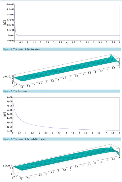
5.2. Simulations

In this part, taking in the system (45), the operator B=I and y0

( )

x = +x 0.3.

(12)

Figure 1.The norm of the free state.

[image:12.595.82.510.75.712.2]

Figure 2.The free state.

Figure 3. The norm of the stabilized state.

(13)

[image:13.595.126.473.80.202.2]

Figure 5. The stabilizing control.

6. Conclusion

In this work, we have considered the problem of strong stabilization with polynomial decay rate of the stabilized state for bilinear parabolic systems that can be decomposed in the stable and unstable parts (15) and (16) under a weaker condition (27). We have also considered the problem of using a stabilizing feedback control for the un-stable part (15) only that can make the whole system (1) un-stable. Various questions remain open. This is the case of stabilization for nonlinear systems. Finally, we have studied the robustness problem of the stabilizing controls with respect to a class of perturbations, but a confrontation to more realistic situations remain done. This leads us to consider the stabilization problem for stochastic bilinear system.

References

[1] Mohler, R.R. (1973) Bilinear Control Process. Academic Press, New York.

[2] Tsouli, A. and Boutoulout, A. (2014) Controllability of the Parabolic System via Bilinear Control. Journal of Dynami-cal and Control Systems, 20, in press. http://dx.doi.org/10.1007/s10883-014-9247-2

[3] Ball, J. and Slemrod, M. (1979) Feedback Stabilization of Distributed Semilinear Control Systems. Applied Mathemat-ics and Optimization, 5, 169-179. http://dx.doi.org/10.1007/BF01442552

[4] Jurdjevic, V. and Quinn, J.P. (1978) Controllability and Stability. Journal of Deferential Equations, 28, 381-389.

http://dx.doi.org/10.1016/0022-0396(78)90135-3

[5] Quinn, J.P. (1980) Stabilization of Bilinear Systems by Quadratic Feedback Control. Journal of Mathematical Analysis and Applications, 75, 66-80. http://dx.doi.org/10.1016/0022-247X(80)90306-6

[6] Ouzahra, M. (2008) Strong Stabilization with Decay Estimate of Semilinear Systems. Systems and Control Letters, 57, 813-815. http://dx.doi.org/10.1016/j.sysconle.2008.03.009

[7] Ouzahra, M., Tsouli, A. and Boutoulout, A. (2012) Stabilization and Polynomial Decay Estimate for Distributed Semi-linear Systems. International Journal of Control, 85, 451-456. http://dx.doi.org/10.1080/00207179.2012.656144

[8] Bounit, H. and Hammouri, H. (1999) Feedback Stabilization for a Class of Distributed Semilinear Control Systems.

Nonlinear Analysis, 37, 953-969. http://dx.doi.org/10.1016/S0362-546X(97)00577-4

[9] Tsouli, A., Ouzahra, M. and Boutoulout, A. (2014) A Decay Estimate for Constrained Semilinear Systems. Information Sciences Letters, 3, 77-83. http://dx.doi.org/10.12785/isl/030206

[10] Chen, M.S. (1998) Exponential Stabilization of a Constrained Bilinear System. Automatica, 34, 989-992.

http://dx.doi.org/10.1016/S0005-1098(98)00037-5

[11] Kato, T. (1980) Perturbation Theory for Linear Operators. Springer, New York.

[12] Ouzahra, M. (2011) Feedback Stabilization of Parabolic Systems with Bilinear Controls. Electronic Journal of Diffe-rential Equations, 38, 1-10.

[13] Triggiani, R. (1975) On the Stabilizability Problem in Banach Space. Journal of Mathematical Analysis and Applica-tions, 52, 383-403. http://dx.doi.org/10.1016/0022-247X(75)90067-0

[14] Pazy, A. (1983) Semi-Groups of Linear Operators and Applications to Partial Deferential Equations. Springer Verlag, New York. http://dx.doi.org/10.1007/978-1-4612-5561-1

[15] Ammari, K. and Tucsnak, M. (2001) Stabilization of Second Order Evolution Equations by a Class of Unbounded Feedbacks. ESAIM: Control, Optimisation and Calculus of Variations, 6, 361-386.

http://dx.doi.org/10.1051/cocv:2001114