Spatial variability in floodplain sedimentation: the use of generalized linear mixed effects models

(1)

www.hydrol-earth-syst-sci.net/14/1655/2010/ doi:10.5194/hess-14-1655-2010

Earth System

Sciences

Spatial variability in floodplain sedimentation: the use of

generalized linear mixed-effects models

A. Cabezas1,2, M. Angulo-Mart´ınez3, M. Gonzalez-Sanch´ıs1, J. J. Jimenez1, and F. A. Com´ın1

1_{Pyrenean Institute of Ecology-Spanish Research Council, IPE-CSIC. 1005 Avd. Monta˜nana, 50080 Zaragoza, Spain} 2_{Leibniz-Institute of Freshwater Ecology and Inland Fisheries, IGB, M¨uggelseedamm 301, 12587 Berlin, Germany}

3_{Aula Dei Experimental Station – Spanish Research Council, EEAD-CSIC. 1005 Avda. Monta˜nana, 50080 Zaragoza, Spain} Received: 10 February 2010 – Published in Hydrol. Earth Syst. Sci. Discuss.: 26 February 2010

Revised: 2 August 2010 – Accepted: 12 August 2010 – Published: 25 August 2010

Abstract. Sediment, Total Organic Carbon (TOC) and to-tal nitrogen (TN) accumulation during one overbank flood (1.15 y return interval) were examined at one reach of the Middle Ebro River (NE Spain) for elucidating spatial pat-terns. To achieve this goal, four areas with different geo-morphological features and located within the study reach were examined by using artificial grass mats. Within each area, 1 m2 study plots consisting of three pseudo-replicates were placed in a semi-regular grid oriented perpendicular to the main channel. TOC, TN and Particle-Size composi-tion of deposited sediments were examined and accumula-tion rates estimated. Generalized linear mixed-effects mod-els were used to analyze sedimentation patterns in order to handle clustered sampling units, specific-site effects and spa-tial self-correlation between observations. Our results con-firm the importance of channel-floodplain morphology and site micro-topography in explaining sediment, TOC and TN deposition patterns, although the importance of other factors as vegetation pattern should be included in further studies to explain small-scale variability. Generalized linear mixed-effect models provide a good framework to deal with the high spatial heterogeneity of this phenomenon at different spatial scales, and should be further investigated in order to explore its validity when examining the importance of factors such as flood magnitude or suspended sediment concentration.

Correspondence to: A. Cabezas ([email protected])

1 Introduction

Riverine floodplains can buffer the transport of sediment as washload mobilised from the upstream parts of the catch-ment. Such sediment deposition over floodplains is an im-portant process in the storage and cycling of sediments, nu-trients and contaminants in the river basins (Walling et al., 1997; Steiger and Gurnell, 2003; Walling and Owens, 2003; Noe and Hupp, 2009). Focussing on organic carbon (TOC) and nitrogen (TN), deposition during overbank floods is an important ecosystem function which provides important ben-efits as water quality enhancement or mitigation of green-house effect (Johnston, 1991; Day et al., 2004; Verhoeven et al., 2006, IPCC, 2007). At the reach scale, TOC and TN exchange between the main channel and its adjacent flood-plain plays a key role in the ecological functioning (Junk, 1999; Robertson et al., 1999; Tockner et al., 1999; Tock-ner at al., 2000; Thoms, 2003; Knosche, 2006; PreiTock-ner et al., 2008). Previous research has shown how human-induced changes at the basin and reach scale have decreased the po-tential of riverine floodplains to act as sediment-associated nutrient sinks (Noe and Hupp, 2005; Owens et al., 2005; Pierce and King, 2008; Cabezas et al., 2009; Cabezas and Comin, 2010). To accomplish knowledge-based manage-ment and restoration strategies at specific river reaches, TOC and TN deposition patterns must be properly understood.

The amounts and patterns of overbank sedimentation de-pend on several factors, namely frequency and duration of inundation, suspended sediment concentration in the main channel, and the flow patterns and stream velocity during floods. Regarding individual events, hydraulic connectiv-ity determines the loading rate of material over floodplains. Hydraulic connectivity, in turn, is controlled at the reach

(2)

1656 A. Cabezas et al.: Spatial variability in floodplain sedimentation scale by channel-floodplain geomorphology, which promotes

spatial variability on sedimentation load and patterns for a given river section during a specific flood event (Hupp, 2000; Steiger and Gurnell, 2003; Noe and Hupp, 2005; Pi´egay et al., 2008). At this scale, previous studies have indicated that distance from the main channel exerts more influence on spa-tial variability of overbank sedimentation than downstream variation (Walling and He, 1998; Middelkoop and Asselman, 1998; Thonon et al., 2007). Such trends were also observed at specific floodplain sections – site-scale – with uniform relief. At more complex sites, however, heterogeneity was strongly related with site micro-topography since it controls flow hydraulics, and thus suspended sediment transport and deposition (Nicholas and Walling, 1997; Hupp et al., 2009). With regards to TOC and TN, the amount of sediment de-posited and particle-size composition seem to determine the TOC and TN deposited in situ during overbank floods (Assel-man and Middelkoop, 1995; Walling and He, 1997; Steiger and Gurnell, 2003).

In this context, different modelling approaches have been employed to predict sedimentation processes and flood ef-fects. Earlier numerical modelling research focussed on dif-fusive sediment and grain-size deposition across channel and floodplain sections (James, 1985; Pizzuto, 1987). By cou-pling hydraulic and sediment deposition models, field-based sedimentation rates and digital elevation models of the flood-plain surface were incorporated to numerical modelling in order to reflect the high spatial heterogeneity observed in field-based investigations. Some of these models are based on a discrete-element approach (Stewart et al., 1998; But-tner et al., 2006), and other models on a finite-element ap-proach (Nicholas and Walling, 1997; Nicholas and Walling, 1998; Middelkoop and Van der Perk, 1998). Those tech-niques advanced the potential to predict sedimentation ef-fects by simple, computationally efficient functions param-eterised by distance from the main channel and floodplain elevation. It also allows the inclusion of the effect of the meso-scale topographic features as abandoned channels, lev-ees or drainage ditches (Nicholas and Mitchell, 2003).

However, empirical studies on contemporary sediment de-position are still needed to gain insight into the key vari-ables that determine spatial heterogeneity (Walling et al., 2004). Despite the complexity of floodplain sedimentation, individual studies rarely incorporate a multi-scale approach when analysing data, although variability at different spatial scales is described and the factors promoting such variability identified. Previous studies have reported high heterogene-ity on floodplain sedimentation (reach scale) when compar-ing sites located within the same study reach (Middlekoop and Asselman, 1998; Walling and He, 1997; Steiger and Gurnell, 2003). Within each site, self-correlation between observation points was observed (site scale). Moreover, self-correlation patterns greatly differed between study sites within the same reach (Middlekoop and Asselman, 1998; Nicholas and Walling, 2003). With regards to smaller scales,

the plot scale variability (∼1 m2)is normally taken into ac-count during the experimental design although not often in-cluded in statistical analyses or spatial interpolation (Mid-delkoop and Asselman, 1998; Steiger and Gurnell, 2003; Steiger et al, 2003).

In the current paper, we aimed to investigate sediment, TOC and TN deposition patterns during one individual flood by considering variability at the reach, site and plot scales. To fulfil our goal, generalized linear mixed-effect models (GLME) represent a potentially useful tool. GLME combine the properties of two statistical frameworks (Bolker et al., 2009): (a) Linear mixed models, which incorporate the ef-fect of random efef-fects; (b) Generalized linear models, which handle nonnormal data by using link functions and the expo-nential family (Poisson, normal, binomial) distributions. By using GLME, hierarchical-data analysis can be performed. GLME represent a class of regression models which do not assume that all observations are independent from each other, and so can be used to analyze data from clustered experimen-tal designs where observed subjects are nested within larger units. By doing so, cluster-specific random effects and cor-related residual structures are included in the analyses (Pin-heiro and Bates, 2000; Heegaard and Nilsen, 2007). Thus, GLME are able to account for differences between flood-plain sections when evaluating floodflood-plain sedimentation in a given reach (reach scale). Self-correlation between obser-vation points lying within the same section (site scale) can be also taken into account by using GLME (Witherington et al., 2009), whereas the small-scale variability (plot scale) is con-sidered without averaging the data. The validity of GLME as a tool to investigate spatial variability in floodplain sedimen-tation studies is also discussed.

2 Materials and methods

2.1 Study reach

(3)

[image:3.595.99.490.63.403.2]

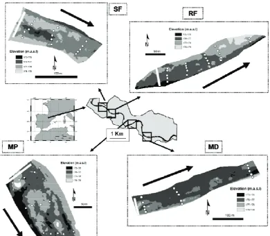
Fig. 1. Location of study plots along the four sites selected within the study reach, which are represented by a detailed Digital Elevation Model. Black arrows indicate the direction of the Ebro River flow. White circles represent the location of the study plots, reflecting an incremental distance to main channel along a perpendicular gradient. White solid lines at each site represent the area where surface water inputs the site, which has been the reference to calculate distances along a longitudinal gradient (see methods).

Table 1. Description of sites where study plots were set.

Site Geomorphological Planform setting Surface Dominant feature of channel bank connectivity land-cover

(m3/s)

MP Point Bar convex 350 Gravel and shrubs

MD Side Channel concave, natural levee 400 Water, grass and trees SF Side Channel convex, natural levee 800 Water, grass and trees

RF Bench convex 600 Grass and shrubs

dominated over natural patch types since 1957, and lateral migration of the main channel has not occurred since 1981 (Cabezas et al., 2009).

2.2 Sediment sampling and analyses

Sediment traps were used to collect the sediment deposited by a 27 days-duration flood on March 2007 (Fig. 2), which

reached 162 m3/s – 1.15 y return interval, 1927–2003; 2.73 y return interval, 1981–2003 – at the Zaragoza gauge station – A011 in www.chebro.es; 12 km upstream from the study area. The sediment traps were placed in four sites with differ-ent geomorphological traits and channel-floodplain connec-tivity – Fig. 1, Table 1: Mejana de Pastriz (MP) and Margen Derecha (MD), with higher channel-floodplain connectivity

[image:3.595.126.467.512.601.2]

(4)

[image:4.595.51.285.60.223.2]

1658 A. Cabezas et al.: Spatial variability in floodplain sedimentation

Fig. 2. Ebro River daily average discharge at the Zaragoza city gauge station during the examined flood. Dot grey line indicates the surface connectivity threshold for MP and MD. Dash grey line indicates the surface connectivity threshold RF. Solid grey line in-dicates the surface connectivity threshold for SF.

than Soto del Franc´es (SF) and Rinc´on Falso (RF). Each area was completely inundated during the examined flood. At each area, 1 m2plots – p=15 at MP, MD and SF; p=22 at RF – were placed in a semi-regular grid, consisting of several tran-sects – t=3 at MP, MD and SF; t=5 at RF – that were oriented perpendicular to the main stream (Fig. 3). The shape and size of each area directed the space between transects and be-tween plots. Study plots were marked by burying a metallic stick, which was geo-referenced using a differential GPS de-vice – Top-Com,±2 cm. In each plot, three 25×25 cm sedi-ment traps – pseudo-replicates – made of artificial grass mats – i=201 – which had been previously weighed, were af-fixed to the surface using 14 cm steel pins. Pseudo-replicates were placed at 30 cm on the left, right and opposite-to-the-river side of the metallic sticks. Sediment traps were set dur-ing the second and third week of February 2006. For each pseudo-replicate, three geographical variables were consid-ered: (i) elevation above sea level (m), extracted from the GPS device measurements; (ii) perpendicular distance (m) to the main channel; and (iii) longitudinal distance, calcu-lated as the distance to the zone where superficial inputs en-ters during overbank floods (Fig. 1), which is located at the upstream part of each site (j=4) and was previously iden-tified from field-based knowledge. Both perpendicular and longitudinal distances were estimated using ArcGIS 9.2

A few days after the flood event, when all of the mats had re-emerged, they were taken to the lab and air-dried at lab temperature during three weeks. Only 3.99% of the artifi-cial grass mats were flushed away by the river. Sedimen-tation rates were calculated as sediment dry mass per area unit (kg/m2)after re-weighing each sediment trap, which had been weighed prior installation. Afterwards, a sediment sam-ple was removed from each trap by hand using a brush with metallic bristles. To ensure homogeneity, mats were brushed

from the centre to the edge covering one quarter. After that, samples were gently mixed by hand. At plots presenting low sedimentation, mats presented great heterogeneity. In these cases, the entire mat was brushed to ensure homogeneity and get enough sediment for further analyses. All sediment sam-ples were finer than 2 mm, so sieving was necessary. Coarse particulate organic matter (>2 mm) was very rare and re-moved when present. An aliquot was separated for particle-size analysis with a laser-diffraction instrument (Coulter LS 230, Beckman Coulter). The <4 µm, <63 µm, <125 µm,

<250 µm and<500 µm particle-size separates were consid-ered for further analyses. These fractions cumulatively repre-sent the clay, silt, and very fine sand, fine sand and medium sand fractions according to Weinthwork (1922). The sed-iment samples were ground with a mortar and pestle prior to measure Total Organic Carbon (TOC) and Total Nitro-gen (TN) using elemental analysis (Leco SC-144DR and El-ementar Variomax CN, respectively). Details on TOC de-termination can be found in Cabezas et al. (2009b). TOC (g C m−2)and TN (g N m−2)accretion rates were calculated multiplying by sedimentation rates.

2.3 Spatial heterogeneity at the reach scale

To describe spatial variability at the reach scale, inter-site (j=4) differences on TOC (%, g C m−2), TN (%, g N m−2), particle size-class separates (%<4, 63, 125, 250, 500 µm) and sedimentation rates (kg m−2)were explored. After en-suring that data met the assumption of normality (including transformations where appropriate), a one-way ANOVA was performed using SPSS 14.0. Depending on the homogeneity of the variance, either SNK or Tahmane Tests were used in post-hoc comparisons.

The existence of spatial self-correlation was tested for the three variables by finding the most appropriate semi-variogram models to fit the empirical semi-semi-variograms com-puted from the samples. The R statistical analysis system – function variogram in the spatial library – (R Develop-ment Core Team, 2008) was used in the calculations. Spa-tial self-correlation was assumed isotropic, since it is one of the main assumptions when including spatial correlation in the GLME models (Pinheiro and Bates, 2000). The Akaike Information Criterion (AIC – Sakamoto, Ishiguro and Kita-gawa, 1986) was used for finding the best semi-variogram model. A Gaussian semi-variogram model was choosen for the sedimentation rate, whereas an Exponential semi-variogram model was applied to TOC and TN deposition. 2.4 Spatial heterogeneity at decreasing spatial scale:

site, transect, row and plot

(5)

FIGURE 3

Fig. 3. Representation of the different spatial scales considered in one of the examined areas (MP, see Fig. 1). The biggest one, the study site scale, encounters the area containing all study plots within a site. The solid rectangle is an example of the area encountered by transects spatial scale, which represents the gradient perpendicular to the main channel. The dashed rectangle is an example of the area encountered by the row spatial scale, which represents the gradi-ent parallel to the main channel. The displayed picture shows the composition of one study plot (solid circle).

sites (Fig. 3). The plot scale represented 1 m2 portions of each study site (3 pseudo-replicates). The transect and row scales (Fig. 3) were selected to assess the spatial variation of sediment deposition in the direction parallel and perpen-dicular to the river. As first pointed by Burrough (1996), this anisotropy on spatial variability is often encountered on river systems. The site scale showed spatial variability within sites –j=4 – with different geomorphological traits. Ar-eas represented by each transect, row and site were identi-fied in the field according to geomorphological traits. Af-terwards, the areas were delimitated over 2003 ortho-images using ArcMap 9.2with a fixed scale of 1:3000, and calculated using the XTools application. Ranges of values at each scale were calculated taking into account sediment traps enclosed at each of the different spatial scales.

Moreover, two different aspects on the relationship be-tween quantity and composition of deposited sediment were evaluated for each site: (i) influence of particle-size sepa-rates over TOC (%) and TN (%) concentrations; (ii) Influ-ence of particle-size separates over sediment (kg m−2), TOC (g C m−2)and TN (g N m−2)deposition rates. To accomplish that, Pearson correlations were performed using SPSS. 2.5 Evaluation of the spatial variability at the reach

scale using GLME modelling

Spatial variability of sediment rate, TOC and TN was as-sessed at the reach scale using generalized linear mixed-effects (GLME) models. Unlike standard linear models, mixed-effects models allow incorporating both fixed-effects and random-effects in the regression analysis (Pinheiro and Bates, 2000). The fixed-effects in a model describe the

val-ues of the response variables in terms of explanatory vari-ables that are considered to be non-random, whereas the random-effects are treated as arising from random causes. Random effects can be associated with the individual ex-perimental units sampled from the population, hence mixed-effects models are particularly suited to experimental settings where measurements are made on groups of related exper-imental units. If the classification factor is ignored when modelling grouped data, the random (group) effects are in-corporated in the residuals, leading to an inflated estimate of the within-site variability.

In our case, relationships were explored between the re-sponse variables – Sedrate, TOC and TN – and the covari-ates – longitudinal and transverse distance to the main chan-nel and percentages of deposited particle size – on a data set grouped according to one classification factor with four lev-els – the four sampling sites: MP, MD, RF and SF . Hence, the mixed-effects model allows for the identification of rela-tionships between the response variables and the covariates that are general to the four sites, irrespective of the local dif-ferences between the sites, which are considered a random effect.

The mixed-effects model combines a random-effects anal-ysis of variance model with a linear regression model. The mathematical formulation takes the form:

yj i=β1+bj+β2xj i+εj ij=1,...,4;i=1,...,201 (1) Whereyj i is the ith observation in the jth group of data and

xj i is the corresponding value of the covariate, an analysis of covariance with a random effect for the intercept; β1 is the mean variable value across the population being sampled,

bj is a random variable representing the deviation from the population mean of the mean variable value for the jth inter-site study area, and

units sampled from the population, hence mixed-effects models are particularly suited to 198

experimental settings where measurements are made on groups of related experimental units. If the 199

classification factor is ignored when modelling grouped data, the random (group) effects are 200

incorporated in the residuals, leading to an inflated estimate of the within-site variability. 201

202

In our case, relationships were explored between the response variables—Sedrate, TOC and TN— 203

and the covariates—longitudinal and transverse distance to the main channel and percentages of 204

deposited particle size—on a data set grouped according to one classification factor with four 205

levels—the four sampling sites: MP, MD, RF andSF . Hence, the mixed-effects model allows 206

finding relationships between the response variables and the covariates that are general to the four 207

sites, irrespective of the local differences between the sites, which are considered a random effect. 208

209

The mixed-effects model combines a random-effects analysis of variance model with a linear 210

regression model. The mathematical formulation takes the form: 211

212

ji ji j

ji b x

y =β1+ +β2 +ε j = 1, …, 4; i = 1, …, 201

213

214

Where yji is the ith observation in the jth group of data and xji is the corresponding value of the 215

covariate, an analysis of covariance with a random effect for the intercept; β1 is the mean variable

216

value across the population being sampled, bj is a random variable representing the deviation from

217

the population mean of the mean variable value for the jth inter-site study area, and Єji is a random

218

variable representing the deviation in the mean variable value for observation i on j from the mean 219

variable value for j on i. 220

221

To complete the statistical model, we must specify the distribution of the random variables bj, j=

222

1,…,4 and Єji, j = 1, …,4; i = 1, …, 201. We begin by modelling both of these as independent,

223

normally distributed random variables with mean zero and constant variance. The variances are 224

denoted σ2b bj, or between site variability, and σ2 for the Єji, or within-site variability. This is

225

expressed as: 226

227

bj, ~N(0, σ2b), Єji ~N(0, σ2)

228 229

Generalized linear mixed-effects (GLME) models allow including a correlation structure to model 230

the spatial dependence between observations. The inclusion of spatial correlation can be achieved 231

by decomposing the within-group variance-covariance structure—Єji—into a product of simpler

232

j iis a random variable representing the deviation in the mean variable value for observationionj

from the mean variable value forj oni.

To complete the statistical model, we must specify the dis-tribution of the random variables bj, j =1,. . . ,4 and

202

209

212

ji ji j

ji b x

y =β1+ +β2 +ε j = 1, …, 4; i = 1, …, 201

213

214

216

217

218

221

222

223

225

expressed as: 226

227

bj, ~N(0, σ2b), Єji ~N(0, σ2)

228 229

232

j i,

j=1, . . . ,4; i=1, . . . , 201. We begin by modelling both of these as independent, normally distributed random vari-ables with mean zero and constant variance. The variances are denotedσ_b2bj, or between site variability, andσ2for the units sampled from the population, hence mixed-effects models are particularly suited to

198

202

209

212

ji ji j

ji b x

y =β1+ +β2 +ε j = 1, …, 4; i = 1, …, 201

213

214

216

217

218

221

222

223

denoted σ2

b bj, or between site variability, and σ2 for the Єji, or within-site variability. This is

225

expressed as: 226

227

bj, ~N(0, σ2b), Єji ~N(0, σ2)

228 229

232

j i, or within-site variability. This is expressed as:

bj,∼N (0,σb2),

202

209

212

ji ji j

ji b x

y =β1+ +β2 +ε j = 1, …, 4; i = 1, …, 201

213

214

216

217

218

221

222

223

denoted σ2

225

expressed as: 226

227

bj, ~N(0, σ2b), Єji ~N(0, σ2)

228 229

232

j i∼N (0,σ2) (2) Generalized linear mixed-effects (GLME) models allow in-cluding a correlation structure to model the spatial depen-dence between observations. The inclusion of spatial cor-relation can be achieved by decomposing the within-group variance-covariance structure –

202

209

212

ji ji j

ji b x

y =β1+ +β2 +ε j = 1, …, 4; i = 1, …, 201

213

214

216

217

218

221

222

223

denoted σ2

225

expressed as: 226

227

bj, ~N(0, σ2b), Єji ~N(0, σ2)

228 229

232

j i – into a product of sim-pler matrices: (i) one describing the variance structure of the within-group errors, (ii) and the other matrix describing the correlation structure of the within-group errors. The spa-tial correlation is represented by its semi-variogram; the type

(6)

1660 A. Cabezas et al.: Spatial variability in floodplain sedimentation of correlation function used to model spatial dependence for

Sedrate, TOC and TN corresponds with the best adjustment achieved when modelling their semi-variogram.

The within-group variance-covariance structure –

202

209

212

ji ji j

ji b x

y =β1+ +β2 +ε j = 1, …, 4; i = 1, …, 201

213

214

216

217

218

221

222

223

225

expressed as: 226

227

bj, ~N(0, σ2b), Єji ~N(0, σ2)

228 229

232

j i– in any model can be assumed to have a homoscedastic within-group error structure, which mean that all within-within-groups er-rors assume the same variance. A more general model al-lows for different variances between study areas and between plots within a study area (heterocedasticity). Heterocedas-ticity can be included in GLME models by means of a vari-ance function. Heteroscesdasticity was evaluated for all three variables – Sedrate, TOC and TN. Several methods exist for fitting GLME models, including maximum likelihood (ML) and restricted maximum likelihood (REML). The R statisti-cal analysis package – function lme from the library nlme – (R Development Core Team, 2008) was used for the gener-alized linear mixed-effectsmodelling. Minimization of the Akaike’s Information Criterion was used for selecting the significant covariates (provided by the function stepAIC of R), as well as for comparing homocedastic and heterocedas-tic models, and choosing between REML and ML fits.

3 Results

3.1 Spatial heterogeneity at the reach scale

Sediment, TOC and TN deposition, as well as related vari-ables (TOC and TN concentration, particle-size separates) showed a high inter-site –j=4 – heterogeneity (Table 2). MP presented the highest sediment deposition rate. In turn, the remaining sites presented higher TOC and TN concentra-tions. Inter-site differences in TOC and TN deposition rates sites diminished when compared with sediment deposition, being the TOC and TN deposition the lowest at RF. With regard to particle-size separates, all fractions<125 µm pre-sented similar inter-site differences than those observed for TOC and TN concentrations, with MP presenting the coars-est deposited sediment. However, particle-size composition did not significantly differ between examined sites regarding the<250 and<500 µm particle-size fractions.

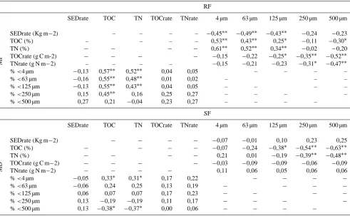
The amount of deposited sediment was related with grain size only at RF (Table 3). At this site, particle-size sepa-rates<125 µm were negatively correlated with the amount of sediment deposited. In turn, those separates>125 µm were negatively correlated with the amount of TOC and TN de-posited. Secondly, particle-size exerted a different influence over TOC and TN concentrations depending on the study site. At MP and RF, TOC and TN concentrations were pos-itively correlated with particle-size separates<125 µm. In turn, TOC and TN concentrations were negatively correlated with the <500 µm particle-size separate at MD, and posi-tively with the<4 µm particle-size separate. At SF, the<250 and<500 µm particle-size separate was negatively correlated with TOC and TN content.

Spatial correlation was significant at distances lower than 0.94 m, 1.30 m, and 1.32 m for Sediment, TOC and TN de-position, respectively. These results evidenced the need of a 1 m2sample grid, at least, as the best structure capturing the spatial heterogeneity in the sediment deposition.

3.2 Spatial heterogeneity at the reach, transect, row and plot scales

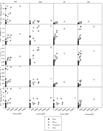
Within the study reach, variability on sediment, TOC and TN deposition was unevenly distributed, as were for TOC and TN concentrations in the deposited sediment (Fig. 4). More-over, variability of these variables (range) increased as their values (magnitude) increase. For Sediment, TOC and TN deposition, heterogeneity was in some cases (MP; MD) as high at the plot scale (1 m2)as it was for the row and transect scales. In turn, heterogeneity on TOC and TN concentration increased when increased sampling area. Within the exam-ined areas, spatial heterogeneity on all examexam-ined variables was as high for the longitudinal gradient as it was for the perpendicular gradient (Fig. 4). Moreover, the study areas, the location of either a plot, transect or row determines its variability on depositional rates, as well as for TOC and TN concentrations. MP presented for depositional rates the high-est site-scale variability for all the study sites. However, all other sites had the highest TOC and TN concentration vari-ability.

3.3 Generalized linear mixed-effects modelling

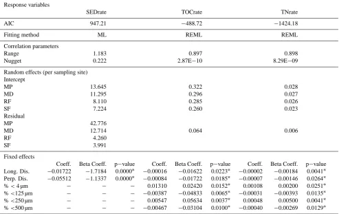
Along the study reach, sediment deposited over the flood-plain decreased with distance perpendicular to the main channel and distance to surface water inputs during the ex-amined flood (Table 4). The random effects were large, as reflected by significant differences in the intercept parameter between sampling sites (Table 4). The GLME model for sed-iment accumulation was the most complex, and included het-eroscesdasticity in the model errors, i.e., when grouping the data by the sampling site, resulting in differences in the resid-uals between sampling sites (Table 4). Fitting was obtained by maximum likelihood (ML). No significant relationship of particle-size composition over the quantity of deposited sed-iment was found. In addition, elevation did not present a significant relationship.

Longitudinal and perpendicular distances were signifi-cantly correlated with TOC and TN deposition rates. The

(7)

[image:7.595.107.485.119.267.2]

Table 2. One-way ANOVA summary results for deposited sediment variables, grouped by study site. All variables presented significant differences except the<250 µm particle-size. Superscript letters (a,b,c) within a row indicate the sub-groups formed after the applied post-hoc comparisons (SNK or Tahmane Test,p <0.05).

Mean±standar error

MP (n=41) MD (n=44) SF (n=44) RF (n=63)

Sedrate (Kg m−2) 13.49±2.19a 5.51±0.53b 4.18±0.27b 4.15±0.38b TOC (%) 0.83±0.05a 1.51±0.09b 1.96±0.07c 1.59±0.07b TN (%) 0.10±0.01a 0.18±0.01b 0.22±0.01c 0.18±0.01b TOC (g C m−2) 112.49±19.52a 77.26±7.91b 78.93±4.08b 56.13±4.36b TN (g N m−2) 11.56±1.67a 8.79±0.83b 9.10±0.46b 6.36±0.44c

<4 µm (%) 2.83±0.16a 4.27±0.22b 5.53±0.26c 4.19±0.22b

<63 µm (%) 24.01±1.43a 32.67±1.43b 40.44±1.39c 31.11±1.24b

<125 µm (%) 43.75±2.20a 50.37±1.78b 57.62±1.45c 48.85±1.30b

<250 µm (%) 74.49±1.84 71.46±1.86 74.57±1.39 71.34±1.03

<500 µm (%) 92.88±0.69a 88.90±1.27b 88.96±0.90b 88.56±0.76b

Table 3. Bivariate correlation between sediment particle-size, carbon and nitrogen concentration and deposition rates (sediment, TOC and TN). Data has been separated by study site: (a) RF, MP; (b) SF, MD. For an easier interpretation, correlations not related to the investigated aspects (see methods) are not displayed.

RF

SEDrate TOC TN TOCrate TNrate 4 µm 63 µm 125 µm 250 µm 500 µm

MP

SEDrate (Kg m−2) – – – – −0,45∗∗ −0,49∗∗ −0,43∗∗ −0,24 −0,23

TOC (%) – – – – 0,53∗∗ 0,43∗∗ 0,25∗ −0,11 −0,30∗

TN (%) − − − − 0,61∗∗ 0,52∗∗ 0,34∗∗ −0,02 −0,20

TOCrate (g C m-2) − − − − −0,15 −0,22 −0,25∗ −0,35∗∗ −0,52∗∗

TNrate (g N m−2) – – – – −0,15 −0,21 −0,23 −0,31∗ −0,47∗∗

%<4 µm −0,13 0,57∗∗ 0,52∗∗ 0,04 0,05 – – – –

%<63 µm −0,16 0,55∗∗ 0,48∗∗ 0,01 0,02 – – –

%<125 µm −0,13 0,55∗∗ 0,43∗∗ 0,04 0,05 – – – –

%<250 µm 0,15 0,45∗∗ 0,16 0,25 0,27 – – – –

%<500 µm 0,27 0,21 −0,04 0,23 0,27 – – – –

SF

SEDrate TOC TN TOCrate TNrate 4 µm 63 µm 125 µm 250 µm 500 µm

MD

SEDrate (Kg m−2) − − − − −0,07 −0,01 0,10 0,23 0,25

TOC (%) − − − − −0,07 −0,24 −0,38∗ −0,54∗∗ −0,63∗∗

TN (%) − − − − 0,21 0,01 −0,19 −0,39∗∗ −0,48∗∗

TOCrate (g C m−2) − − − − −0,03 −0,09 −0,09 −0,06 −0,09

TNrate (g N m−2) − − − − 0,11 0,06 0,05 0,06 0,06

%<4 µm −0,05 0,33∗ 0,31∗ 0,17 0,22 − − − −

%<63 µm −0,06 0,24 0,25 0,13 0,19 − − − −

%<125 µm 0,06 0,07 0,07 0,17 0,23 − − − −

%<250 µm 0,13 −0,19 −0,19 0,11 0,17 − − − −

%<500 µm 0,13 −0,38∗ −0,37∗ 0,00 0,06 − − − −

∗_{= Correlation is significant at the 0.05 level (2-tailed).} ∗∗_{= Correlation is significant at the 0.01 level (2-tailed).}

[image:7.595.52.544.340.643.2]

(8)

[image:8.595.119.481.67.527.2]

Fig. 4. TOC (%, g C m−2), TN (%, g N m−2) and sedimentation rates (kg/m2) ranges for different spatial scales (plot, transect, row and site).

See methods for details on area calculations.

heterocedastic models for TOC and TN deposition. AIC also indicated that RMLE was the best method to fit the TOC and TN heterocedastic models by using the AIC. Neither the

<63 µm nor the elevation were estimated as significant and therefore not included in the model.

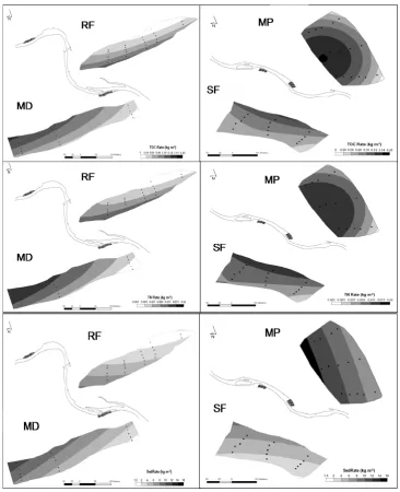
Coefficients to generate maps of predicted sediment rate, TOC and TN (Fig. 5) were obtained from the GLME mod-els. As expected from the previous description, these maps reflect a high degree of spatial heterogeneity at the reach and site scales. As the fixed effects showed, the highest values of deposited sediment, TOC and TN in each sampling site were found close to the main channel and at the upstream

end of the site. Differences between sites in the average sed-iment rate were large, the highest amounts occurring at MP and MD sites whereas lower values were predicted at SF and RF sites. For all sites, the predicted values reflect how sedi-ment deposition decreases whit increasing distance from the main channel and upstream inputs, both of which are sedi-ment sources.

(9)

[image:9.595.51.545.144.455.2]

Table 4. Summary of the results of the generalized linear mixed-effects models for sedimentation rate (SEDrate), Total Organic Carbon (TOCrate) and Total Nitrogen (TNrate): Goodness of fit statistic value (AIC); Fitting method: Maximum Likelihood (ML) or Restricted Maximum Likelihood (REML); Correlation parameters; Random effects for sampling site and model corresponding to the intercept and, in the case of heterocedasticity, in the residuals; Coefficients of the fixed effects: Coeff., Beta Coeff. (standarized coefficients) and p-values for the sedimentation rate (SEDrate), Total Organic Carbon (TOCrate) and Total Nitrogen (TNrate) models. Long. Dis. = Longitudinal distance; Perp. Dis. = Perpendicular distance (see methods for details).

Response variables

SEDrate TOCrate TNrate

AIC 947.21 −488.72 −1424.18

Fitting method ML REML REML

Correlation parameters

Range 1.183 0.897 0.898

Nugget 0.222 2.87E−10 8.29E−09

Random effects (per sampling site) Intercept

MP 13.645 0.322 0.028

MD 11.295 0.296 0.027

RF 8.110 0.285 0.026

SF 7.224 0.260 0.023

Residual

MP 42.776

MD 12.714 0.064 0.006

RF 4.260

SF 3.991

Fixed effects

Coeff. Beta Coeff. p−value Coeff. Beta Coeff. p−value Coeff. Beta Coeff. p−value Long. Dis. −0.01722 −1.7184 0.0000∗ −0.00016 −0.01622 0.0223∗ −0.00002 −0.00184 0.0041∗ Perp. Dis. −0.05512 −1.1337 0.0000∗ −0.00084 −0.01722 0.0185∗ −0.00007 −0.00146 0.0264∗

%<4 µm − − − 0.01310 0.02420 0.0152∗ 0.00108 0.00200 0.0251∗

%<125 µm − − − −0.00387 −0.04833 0.0065∗ −0.00031 −0.00393 0.0135∗

%<250 µm − − − 0.00547 0.05634 0.0037∗ 0.00048 0.00500 0.0041∗

%<500 µm − − − −0.00467 −0.03104 0.0100∗ −0.00040 −0.00269 0.0129∗

due to the existence in the model of covariates other than the distance to the river. Differences in the mean TOC and TN concentrations between were significantly lower than differ-ences in sediment rate between sites.

4 Discussion

4.1 Spatial heterogeneity at different scales

Spatial heterogeneity at the reach scale (10 000–100 000 m2)

influenced site-scale heterogeneity (1000–10 000 m2) by limiting the variation range at the examined sites (Fig. 4). It occurred for the amount of sediment, TOC and TN de-posited, as well as for TOC and TN concentrations. However, limitation of spatial heterogeneity at the plot scale (1 m2)by the site scale heterogeneity (1000–10 000 m2)was not clear. Regarding the amount of sediment, TOC and TN deposited, the plot scale heterogeneity can be as high as it was for big-ger spatial scales as row or transect. Regarding TOC and

TN concentrations, variability increase along with the spatial scale, and so with the extent of the examined area.

The relationship between the amount of sediment de-posited and its particle-size composition varied when consid-ering different spatial scales. Sediment deposition was neg-atively correlated at the reach scale with the proportion of the finest sediment fractions (%<4, 63, 125 µm; p <0.01,

n=201), whereas positively correlated with the %<500 µm particle-size separate (p <0.01,n=201). This is similar to the reach-scale results of Steiger and Gurnell (2003). How-ever, when analyzing the data at the site scale, we noted that this negative relationship at the reach scale was only found to exist at the RF site (Table 3), in agreement with results from Walling and He (1998) who found also no relation-ship between sediment deposition and grain size at the site scale. They highlighted the need to recognise that the sus-pended sediment transported by a river is commonly trans-ported as aggregates rather than individual particles. In ad-dition, convective transport processes could explain these

(10)

1664 A. Cabezas et al.: Spatial variability in floodplain sedimentation trends (Asselman and Midlekoop, 1995). In turn, the

reach-scale relationships between TOC and TN concentrations on deposited sediments and particle size composition remained relatively stable when down-scaling to the site-scale. TOC and TN concentrations were positively correlated (Table 3) with the proportion of the finest sediment fraction at the reach scale (%<4, 63, 125 µm;p <0.01,n=201), whereas they were negatively correlated with the medium sand size frac-tion (% <500 µm; p <0.01, n=201). At the site scale, the importance of each fraction varied depending on the site. Positive relationships with the percentage of<63 µm particle-size separate have been previously reported (Walling and He, 1997; Steiger and Gurnell, 2003), although are pro-vided for the remainder fractions in these papers.

At the reach scale, channel-floodplain geomorphology promoted heterogeneity on the amount and composition of sediment retained during the examined flood (Table 2). This trend has been previously observed in other studies deal-ing with contemporary sedimentation rates (Middlekoop and Van der Perk, 1998; Nicholas and Walling, 1998; Thonon et al., 2007). River-floodplain connectivity governs hydraulic patterns of overbank flows, and thus sedimentation patterns. Flooding took place later and was shorter at sites with the lower superficial connectivity thresholds (SF and RF in Ta-bles 1 and 2), where sedimentation rates were the lowest. Moreover, a decrease on the amount of suspended sedi-ment during the flood (Asselman and Middlekoop, 1998; Baborowski et al., 2007), which is higher at initial stages, could decrease the amount of sediment deposited at these sites. In turn, the proportion of the finest particle-size sep-arates, i.e. <125 µm (fine sand) increased at those sites. Assuming homogeneity of suspended sediment composition within the study reach, it would result from a drastic decrease of flow velocity at main channel margins. As a result, the coarsest particles, which are normally transported by diffu-sive processes (Asselman and Middlekoop, 1995; Walling and He, 1998), are released before water enters the flood-plain. Such phenomenon could also underlay results at MD, the high-connected side channel. At MD, the amount of sed-iment deposited was slightly higher than in low-connected sites. The location of MD in the concave bank of a river me-ander could reduce the quantity of sediment deposited by in-creasing erosion at certain flood stages (Steiger and Gurnell, 2003). At the other high-connected site, MP, extraordinary high sedimentation rates of coarse sediment were estimated. MP is characterized by a smooth topographic change at the border with the main channel.

At the site scale, complexity of local topography cre-ates complex sedimentation patterns (Walling and He, 1998; Hupp et al., 2009). Spatial differences in sedimentation de-pend, at first, on the distance to water and sediment inputs (Table 4). Secondly, local topography attributes as relict channels create preferential flowpaths along which particles and aggregates are conveyed. Depletion of suspended sedi-ment by sedisedi-mentation along preferential flow paths results

(Middelkoop and Van der Perk, 1998). At the examined sites, sediment, TOC and TN deposition varied along gradients which run parallel and perpendicular to the main channel (Fig. 5). Therefore, it is reasonable to assume that deposi-tion from sediment entering the floodplain at the upstream area is as important as those entering adjacent areas to the main channel. Moreover, variability within these gradients can differ depending on the location of the area within the same study site. This implies that either suspended sedi-ment concentrations decreased along flowpaths, or sedisedi-ment is transported by convective processes further from the input point.

At the plot scale (1 m2), further research is required to elu-cidate factors promoting variability on the considered vari-ables. Spatial heterogeneity may respond to heterogeneous vegetation structure within each plot, which modifies flow patterns and therefore result on differences on sediment de-position. Nicholas and Walling (1997) highlighted the need to include such effects on sedimentation modelling in order to improve its predictive ability at small spatial scales. Al-though factors promoting variability at the plot scale were not identified, our results indicate that the plot scale vari-ability was smaller for TOC and TN concentrations that for the amount of sediment deposited (Fig. 4). This suggest that there is a certain degree of homogeneity in suspended sed-iment composition when a given floodplain area is flooded, and indicates that factors promoting heterogeneity at the plot scale mainly operate over the amount sediment which is de-posited. In turn, factors promoting heterogeneity at larger spatial scales influenced TOC and TN concentrations. Re-sults from the present study indicate that the amount of TOC and TN deposited depend on sediment quantity rather than in their TOC and TN contents (Table 2), in agreement with previous reports in this study reach (Cabezas et al., 2009). Consequently, studies dealing with TOC and TN retention by floodplain habitats should address influence of these hot spots. The crucial role of hot spots on TOC and TN reten-tion has been previously highlighted for other biogeochemi-cal processes implied in the TOC and TN turnover at riparian floodplains (McClain et al., 2003; Groffman et al., 2009). 4.2 Linear mixed-effect models

(11)

[image:11.595.114.481.63.514.2]

Fig. 5. Prediction maps sediment, TOC and TN deposition after the Generalized linear mixed-effects models.

of TOC, TN and deposition rate, independent of the site con-sidered. The validity of our model at another Middle Ebro River reaches with similar geomorphological features is pos-sible although must be investigated. However, a development of a new model which includes different-magnitude flood events is necessary to generalize our findings at larger tem-poral scales. Moreover, GLME handles small-scale hetero-geneity by including all sampling units (pseudo-replicates) at each study plot. Previous studies (Steiger and Gurnell, 2003; Steiger et al., 2003) applied a lumped approach by av-eraging values of the clustered sampling units. According to our models, the amount of deposited sediment, TOC and TN decreases within the study reach with distance to

superfi-cial water inputs (longitudinal and perpendicular distance in Table 4). The inverse relationship between elevation and sed-imentation rate (Walling et al., 1996; Walling and He, 1998) could not be confirmed by this study. As Middelkoop and As-selman (1998) and Thonon et al. (2007b) found, this might be attributed to levees and other topographic features. More-over, high flow velocities at low-lying areas can even reverse this trend at certain flood magnitudes (Asselman and Mid-dlekoop, 1998). The inclusion of the particle size fractions in the TOC and TN deposition models reflects the influence that particle-size exerted on sediment composition at the four examined sites (Table 4). Assignation of model coefficients to the different particle-size classes respond to the best model

(12)

1666 A. Cabezas et al.: Spatial variability in floodplain sedimentation goodness of fit and not to the previously described

empiri-cal relationships. Note that cumulative particle-size fractions were considered for this study.

Secondly, GLME models are able to predict Sediment, TOC and TN deposition at the reach scale taking into ac-count spatial heterogeneity at smaller spatial scales. As a result, predicted deposition maps could be built for the four study sites included in the analyses (Fig. 5). To interpret predicted patterns, knowledge on site-specific features is re-quired, as it was required by previous studies evaluating floodplain sedimentation by using different techniques than those performed in the current study (Middelkoop and As-selman, 1998; Steiger and Gurnell, 2003). However, GLME models are a useful tool when the scope of the study is to predict Sediment, TOC and TN deposition at heterogeneous river reaches rather than explaining spatial patterns at the site scale. At the study reach scale, homogeneity of spatial pat-terns was higher than expected for three of the four sites ex-amined (Fig. 4). Flood magnitude and duration probably de-termined sediment deposition patterns at the examined sites. Also the position of study plots only in areas adjacent to the channel margin could influence the results. Future studies (either during different lower magnitude floods or position-ing study plots in areas far to the main channel) are required to test the validity of our findings at spatio-temporal scales different than those considered in this study.

5 Conclusions

In the current paper, Sediment, TOC and TN deposition in one reach of the Middle Ebro River were evaluated by using GLME models. From this, we conclude:

1. As previously described for other study areas, channel-floodplain connectivity determines spatial heterogeneity on floodplain sedimentation at the reach scale, whereas micro-topography controls at the site scale.

2. Relationships between the amount of sediment de-posited and its characteristics (particle size, TOC and TN concentration) vary when considering different spa-tial scales.

3. Sediment deposition variability at the plot scale (1 m2)

can be as high as is for larger spatial scales (1000– 10 000 m2). This should be considered in future studies. 4. Factors determining heterogeneity at the plot scale ex-ert a higher influence over the amount of sediment de-posited than over TOC and TN concentrations.

5. By considering random effects, GLME can elucidate which variables were significant in controlling the spa-tial sedimentation patterns of TOC, TN and deposition rate, independent of the site considered. Thus, con-clusions could be extrapolated with caution to different study sites.

6. GLME is a useful tool when the scope of the study is predicting Sediment, TOC and TN deposition at the reach scale while taking into account heterogeneity at smaller spatial scales.

Acknowledgements. Field works were funded by the

Depart-ment of EnvironDepart-mental Science, Technology and University – Government of Aragon (Research group E-61 on Ecological Restoration)– and MEC (CGL2005-07059). The Spanish Research Council (CSIC) granted ´Alvaro Cabezas through the I3P program (I3P-EPD2003-2), which was financed by European Social Funds (UE). Thanks are extended to Melchor Maestro for his help with the TN analyses. Research of M. Angulo-Mart´ınez is supported by a JAE-Predoc Research Grant from the Spanish National Research Council (Consejo Superior de Investigaciones Cient´ıficas – CSIC).

Edited by: M. Gooseff

References

Asselman, N. E. M. and Middelkoop, H.: Floodplain Sedimentation – Quantities, Patterns and Processes, Earth. Surf. Proc. Land., 20, 481–499, 1995.

Asselman, N. E. M. and Middelkoop, H.: Temporal variability of contemporary floodplain sedimentation in the Rhine-Meuse Delta, the Netherlands, Earth. Surf. Proc. Land., 23, 595–609, 1998.

Baborowski, M., Buttner, O., Morgenstern, P., Kruger, F., Lobe, I., Rupp, H., and Von Tumpling, W. V.: Spatial and temporal vari-ability of sediment deposition on artificial-lawn traps in a flood-plain of the River Elbe, Environ. Manage., 48, 770–778, 2007. Bolker, B. M., Brooks, M. E., Clark, C. J., Geange, S. W., Poulsen,

J. R., Stevens, M. H. H., and White, J. S. S.: Generalized lin-ear mixed models: a practical guide for ecology and evolution, Trends Ecol. Evol., 24, 127–135, 2009.

Buttner, O., Otte-Witte, K., Kruger, F., Meon, G., and Rode, M.: Numerical modelling of floodplain hydraulics and suspended sediment transport and deposition at the event scale in the mid-dle river Elbe, Germany, Acta Hydroch. Hydrob., 34, 265–278, 2006.

Cabezas, A., Comin, F. A., Begueria, S., and Trabucchi, M.: Hy-drologic and landscape changes in the Middle Ebro River (NE Spain): Implications for restoration and management, Hydrol. Earth Syst. Sci., 13, 273–284, 2009,

http://www.hydrol-earth-syst-sci.net/13/273/2009/.

Cabezas, A., Comin, F. A., and Walling, D. E.: Changing patterns of organic carbon and nitrogen accretion on the middle Ebro flood-plain (NE Spain), Ecol. Eng., 35, 1547–1558, 2009b.

Cabezas, A. and Comin, F. A.: Carbon and nitrogen accretion in the topsoil of the Middle Ebro River Floodplains (NE Spain): Implications for their ecological restoration, Ecol. Eng., 36, 640– 652, 2010.

(13)

Heegaard, E. and Nilsen, T.: Local linear mixed effect models – Model specification and interpretation in a biological context, J. Agric. Biol. Envir. S., 12, 414–430, 2007.

Hupp, C. R.: Hydrology, geomorphology and vegetation of Coastal Plain rivers in the south-eastern USA, Hydrol. Process., 14, 2991–3010, 2000.

Hupp, C. R., Pierce, A. R., and Noe, G. B.: Floodplain geomorphic processes and environmental impacts of human alterations along coastal plain rivers, USA. Wetlands., 29, 413–429, 2009. IPCC: Working Group III Report “Mitigation of Climate Change”,

Cambridge Univeristy Press, Cambridge, United Kingdom., 2007.

James, C. S.: Sediment transfer to overbank sections, J. Hydrol. Res., 23, 435–452, 1985.

Johnston, C. A.: Sediment and nutrient retention by freshwater wet-lands – Effects on surface-water quality, Crit. Rev. Env. Contr., 21, 491–565, 1991.

Junk, W. J.: The flood pulse concept of large rivers: learning from the tropics, Arch. Hydrobiol., 3, 261–280, 1999.

Knosche, R.: Organic sediment nutrient concentrations and their re-lationship with the hydrological connectivity of floodplain waters (River Havel, NE Germany), Hydrobiologia, 560, 63–76, 2006. Middelkoop, H. and Asselman, N. E. M.: Spatial variability of

floodplain sedimentation at the event scale in the Rhine-Meuse delta, the Netherlands, Earth Surf. Proc. Land., 23, 561–573, 1998.

Middelkoop, H. and Van der Perk, M.: Modelling spatial patterns of overbank sedimentation on embanked floodplains, Geogr. Ann. A., 80A, 95–109, 1998.

Nicholas, A. P. and Walling, D. E.: Modelling flood hydraulics and overbank deposition on river floodplains, Earth Surf. Proc. Land., 22, 59–77, 1997.

Nicholas, A. P. and Walling, D. E.: Numerical modelling of flood-plain hydraulics and suspended sediment transport and deposi-tion, Hydrol. Proces., 12, 1339–1355, 1998.

Nicholas, A. P. and Mitchell, C. A.: Numerical simulation of over-bank processes in topographically complex floodplain environ-ments, Hydrol. Proces., 17, 727–746, 2003.

Noe, G. B. and Hupp, C. R.: Carbon, nitrogen, and phosphorus ac-cumulation in floodplains of Atlantic Coastal Plain rivers, USA, Ecol. Appl., 15, 1178–1190, 2005.

Noe, G. B. and Hupp, C. R.: Retention of Riverine Sediment and Nutrient Loads by Coastal Plain Floodplains, Ecosystems, 12, 728–746, 2009.

Ollero, A.: Din´amica reciente del cauce de el Ebro en la Reserva Natural de los Galachos, Cuat. Geomor., 9, 85–93, 1995. Owens, P. N., Batalla, R. J., Collins, A. J., Gomez, B., Hicks, D.

M., Horowitz, A. J., Kondolf, G. M., Marden, M., Page, M. J., Peacock, D. H., Petticrew, E. L., Salomons, W., and Trustrum, N. A.: Fine-grained sediment in river systems: Environmental significance and management issues, River Res. Appl., 21, 693– 717, doi:10.1002/rra.878, 2005.

Piegay, H., Hupp, C. R., Citterio, A., Dufour, S., Moulin, B., and Walling, D. E.: Spatial and temporal variability in sedimentation rates associated with cutoff channel infill de-posits: Ain River, France, Water Resour. Res., 44, W05420, doi:10.1029/2006WR005260, 2008.

Pierce, A. R. and King, S. L.: Spatial dynamics of overbank sedi-mentation in floodplain systems, Geomorphology, 100, 256–268,

2008.

Pinheiro, J. C. and Bates, D. M.: Mixed-Effects Models in S and S-PLUS, Springer, New York, 530 pp., 2000.

Pizzuto, J. E.: Sediment diffusion during overbank flows, Sedimen-tology, 34, 301–317, 1987.

Preiner, S., Drozdowski, I., Schagerl, M., Schiemer, F., and Hein, T.: The significance of side-arm connectivity for carbon dynam-ics of the River Danube, Austria, Freshwater Biol., 53, 238–252, 2008.

Robertson, A. I., Bunn, S. E., Boon, P. I., and Walker, K. F.: Sources, sinks and transformations of organic carbon in Aus-tralian floodplain rivers, Mar. Freshwater Res., 50, 813–829, 1999.

Sakamoto, Y., Ishiguro, M., and Kitagawa, G.: Akaike Information Criterion Statistics, Reidel, Dordrecht, Holland., 1986.

Steiger, J. and Gurnell, A. M.: Spatial hydrogeomorphological in-fluences on sediment and nutrient deposition in riparian zones: observations from the Garonne River, France, Geomorphology, 49, 1–23, 2003.

Steiger, J., Gurnell, A. M., and Goodson, J. M.: Quantifying and characterizing contemporary riparian sedimentation, River Res. Appl., 19, 335–352, 2003.

Stewart, M. D., Bates, P. D., Price, D. A., and Burt, T. P.: Mod-elling the spatial variability in floodplain soil contamination dur-ing flood events improve chemical mass balance estimates, in: Hihg-Resolution Modelling in Hydrology and Geomorphology, edited by: Bates, P. D. and Lane, S. D., Wiley, Chichester, 239– 261, 1999.

R development core team, R: A language and Environment for Sta-tistical Computing, Foundation fro StaSta-tistical Computing, (http: //www.R-project.org), Vienna, Austria. 2008.

Thonon, I., de Jong, K., van der Perk, M., and Middelkoop, H.: Modelling floodplain sedimentation using particle tracking, Hy-drol. Process., 21, 1402–1412, 2007.

Thonon, I., Middelkoop, H., and van der Perk, M.: The influence of floodplain morphology and river works on spatial patterns of overbank deposition, Neth. J. Geosci., 86, 63–75, 2007b. Thoms, M. C.: Floodplain-river ecosystems: lateral connections

and the implications of human interference, Geomorphology, 56, 335–349, 2003.

Tockner, K., Pennetzdorfer, D., Reiner, N., Schiemer, F., and Ward, J. V.: Hydrological connectivity, and the exchange of or-ganic matter and nutrients in a dynamic river-floodplain system (Danube, Austria), Freshwater Biol., 41, 521–535, 1999. Tockner, K., Malard, F., and Ward, J. V.: An extension of the flood

pulse concept, Hydrol. Process., 14, 2861–2883, 2000.

Verhoeven, J. T. A., Arheimer, B., Yin, C. Q., and Hefting, M. M.: Regional and global concerns over wetlands and water quality, Trends Ecol. Evol., 21, 96–103, 2006.

Walling, D. E., He, Q., and Nicholas, A. P.: Floodplains as Sus-pended Sediment Sinks, in: Floodplain Processes, edited by: An-derson, G. M., Walling, D. E., and Bates, P. D., Wiley, Chich-ester, 399–440, 1996.

Walling, D. E. and He, Q.: Investigating spatial patterns of overbank sedimentation on river floodplains, Water Air Soil Poll., 99, 9– 20, 1997.

Walling, D. E., Owens, P. N., and Leeks, G. J. L.: The character-istics of overbank deposits associated with a major flood event in the catchment of the River Ouse, Yorkshire, UK, Catena, 31,

(14)

53–75, 1997.

Walling, D. E. and He, Q.: The spatial variability of overbank sed-imentation on river floodplains, Geomorphology, 24, 209–223, 1998.

Walling, D. E. and Owens, P. N.: The role of overbank floodplain sedimentation in catchment contaminant budgets, Hydrobiolo-gia, 494, 83–91, 2003.

Walling, D. E.: Quantifying the fine sediment budgets of river basins., Proceedings Irish National Hydrology Seminar, 9–20, 2004.

Wentworth, C. K.: A scale of grade and class terms for clastic sedi-ments. J. Geol., 30, 377–350, 1922.