www.hydrol-earth-syst-sci.net/19/4365/2015/ doi:10.5194/hess-19-4365-2015
© Author(s) 2015. CC Attribution 3.0 License.
Process verification of a hydrological model using a temporal
parameter sensitivity analysis
M. Pfannerstill1, B. Guse1, D. Reusser2, and N. Fohrer1
1Christian-Albrechts-University of Kiel, Institute of Natural Resource Conservation, Department of Hydrology and Water Resources Management, Kiel, Germany
2Potsdam Institute for Climate Impact Research, Potsdam, Germany
Correspondence to: M. Pfannerstill ([email protected])
Received: 11 December 2014 – Published in Hydrol. Earth Syst. Sci. Discuss.: 5 February 2015 Revised: 4 October 2015 – Accepted: 7 October 2015 – Published: 29 October 2015
Abstract. To ensure reliable results of hydrological models, it is essential that the models reproduce the hydrological cess dynamics adequately. Information about simulated pro-cess dynamics is provided by looking at the temporal sensi-tivities of the corresponding model parameters. For this, the temporal dynamics of parameter sensitivity are analysed to identify the simulated hydrological processes. Based on these analyses it can be verified if the simulated hydrological pro-cesses match the observed propro-cesses of the real world.
We present a framework that makes use of processes ob-served in a study catchment to verify simulated hydrolog-ical processes. Temporal dynamics of parameter sensitivity of a hydrological model are interpreted to simulated hydro-logical processes and compared with observed hydrohydro-logical processes of the study catchment. The results of the analysis show the appropriate simulation of all relevant hydrological processes in relation to processes observed in the catchment. Thus, we conclude that temporal dynamics of parameter sen-sitivity are helpful for verifying simulated processes of hy-drological models.
1 Introduction
Discharge, one of the major outputs of hydrological models, is controlled by a number of interacting processes. However, a simple comparison of observed and simulated discharge, which is often the only criterion used for model calibration and evaluation, does not take into account the underlying pro-cesses that shape the hydrograph. For a more profound as-sessment of the reliability of model results, a deeper
under-standing of how these processes are described in the model and a more detailed analysis of how well the corresponding real-world processes are represented are essential. To deter-mine if the model behaviour is consistent with the hydrolog-ical processes observed in a catchment, the model structure, i.e. the model equations and parameters, needs to be con-sidered when evaluating the model output (e.g. Gupta et al., 2008; Hrachowitz et al., 2014).
Model diagnostic analyses as proposed by Gupta et al. (2008) and Yilmaz et al. (2008) determine the appropriate-ness of process descriptions in the model structure. Thus, di-agnostic methods help to detect failures in models and the corresponding components that need to be improved (Feni-cia et al., 2008; Reusser and Zehe, 2011; Guse et al., 2014).
As stated by Yilmaz et al. (2008), a systematic approach to analysing the adequacy of model structures is needed, since the processes occurring in a catchment are not always represented appropriately within hydrological models (Clark et al., 2011). There is a need to assess if the model struc-tures and the simulated processes are consistent with ob-served hydrological processes within the catchment (Gupta et al., 2012). This is a step towards establishing a general framework for model accuracy verification (Wagener et al., 2001; Yilmaz et al., 2008).
output or similarity between the functioning of the model and the hydrologic system it describes.
Temporal parameter sensitivity analyses detect periods in which a certain parameter or a set of parameters controls the model output (e.g. Massmann et al., 2014). This informa-tion can be obtained by TEmporal Dynamics of PArameter Sensitivity (TEDPAS, Sieber and Uhlenbrook, 2005; Reusser et al., 2011; Guse et al., 2014; Haas et al., 2015).
In contrast to other temporally resolved sensitivity anal-yses, which were applied on performance metrics (van Werkhoven et al., 2009; Herman et al., 2013), TEDPAS de-tects dominant model parameters by analysing their sensi-tivity on the modelled discharge in a high temporal resolu-tion. Thereby, it helps to explain the model’s behaviour by detecting the temporal dominance of individual model com-ponents. Reusser et al. (2009) used TEDPAS in combina-tion with TIGER, a temporal model performance analysis (Reusser et al., 2009), to characterise the types of errors in the output of hydrological models (e.g. the simulation of dis-charge). Wagener et al. (2003) analysed parameter variations over time to reproduce observed hydrological data. Both ap-proaches have in common that they focus on the link between model performance and deficiencies of the model structure. However, the capabilities of TEDPAS for examining model structures have not been fully exploited yet.
Typical patterns of temporal parameter sensitivity can pro-vide information about simulated hydrological processes. This approach is based on the fact that hydrological pro-cesses and discharge phases vary temporally and hence also the dominance of model components (Boyle et al., 2000, 2001; Wagener et al., 2003, 2009; Reusser et al., 2011; Garambois et al., 2013; Guse et al., 2014).
In this context, Guse et al. (2014) used TEDPAS and TIGER to detect which component of a hydrological model was responsible for poorly simulated baseflow in dry years. Although the temporal variability of the parameter sensitiv-ity was reasonable, the model performed poorly for several performance metrics in phases of groundwater dominance (Guse et al., 2014). Based on this temporal diagnostic anal-ysis, Pfannerstill et al. (2014a) modified the aquifer struc-ture of the model to emphasise non-linear dynamics of the groundwater processes. The analysis of Pfannerstill et al. (2014b) showed that the modification improved the simula-tion of the discharge with respect to different performance metrics. However, an analysis of the hydrological processes and their representation by the model structure is required to prove that the simulation of discharge was improved for the right reasons (Kirchner, 2006).
Therefore, this study aims at developing a method that ver-ifies appropriate process simulation of hydrological models using TEDPAS and observed hydrological processes of the study catchment. Based on an application example, we pro-pose a general framework for the verification of hydrological consistency of models that is in principal applicable to any model in any catchment.
TEDPAScatchment
the results of TEDPAS for the hydrological model
aiming to verify...
to derive hypotheses... about thesequence of observed processes
Uses... observations and knowledge of the catchment
and uses...
agreement betweensequences of simulatedandobserved processes to extract... thesequence of simulated processes a)
b)
c)
d)
[image:2.612.308.549.67.342.2]e)
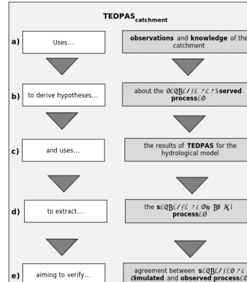
Figure 1. General idea of TEDPAScatchmentas a verification frame-work. The framework integrates processes observed in the catch-ment (a) to derive hypotheses about the temporal sequence of ob-served processes (b) and the calculation of temporal parameter sen-sitivities with TEDPAS, (c) to extract the temporal sequence of sim-ulated processes (d) for the investigated hydrological model. The verification of the model is performed by comparing the temporal sequences of observed and simulated processes (e).
We demonstrate how to (i) use observed hydrological pro-cesses of a catchment for (ii) comparison with TEDPAS re-sults to (iii) verify that processes are adequately simulated by a hydrological model.
2 Methods
The general idea of the proposed framework is to make use of processes observed within the catchment and results of TEDPAS to verify hydrological models (Fig. 1). For this, all available information about processes occurring in the study catchment is collected (Fig. 1a). These processes are then ordered according to the timing of their occurrence, which is controlled by seasonal hydrological conditions. Hypotheses about assumed process dynamics are formulated based on this temporal sequence of observed processes (Fig. 1b).
the model behaviour, there is no need for previous model calibration. In principle, the central aim of TEDPAS is not to provide direct information of how to define model param-eters in a calibration of a hydrological model, but rather to derive information about the behaviour of model parameters over time (Fig. 1c). The temporal dynamics of parameter sen-sitivity are used to draw inferences to hydrological processes. In a similar manner, the temporal sequence of simulated pro-cesses is derived from the timing of simulated hydrological processes (Fig. 1d).
Since the sequences of observed and simulated processes both describe the timing of hydrological processes, they are directly comparable to each other. An appropriate simulation of the hydrological processes is then verified by comparing the temporal sequences of observed and simulated processes (Fig. 1e). Consequently, the hydrological consistency in rep-resenting the whole hydrological system is investigated (e.g. Martinez and Gupta, 2011; Euser et al., 2013). In the fol-lowing, the individual methods that are part of the proposed framework are described in detail.
2.1 Processes observed in the catchment
To achieve hydrologically consistent model results, the model should be able to simulate all relevant hydrologi-cal processes of the study catchment. Therefore, knowledge about observed hydrological processes is crucial to evaluate the hydrological consistency of the model results. For this, all available information available from previous field stud-ies and general knowledge about hydrological characteristics of the study catchment needs to be collected (Fig. 1a). This information is then used to identify all relevant hydrologi-cal processes of the study catchment and the timing of their occurrence.
2.2 Derived hypotheses
The knowledge about processes observed in the catchment is translated into information that is comparable with pro-cesses simulated by the model. For this, qualitative hypothe-ses about seasonal process occurrences, process dynamics and specific hydrological situations observed in the catch-ment are formulated (Fig. 1b). Each hypothesis incorporates knowledge such as the activity of tile drainages, the seasonal groundwater contribution to the total discharge or the impact of soil water dynamics on surface runoff. However, it has to be emphasised that the incorporated hydrological informa-tion needs to be derived from observed data of the catchment (Fig. 1a). In this way, real-world processes are considered for the verification framework.
2.3 TEDPAS methods
TEDPAS was selected to provide the temporal sequence of simulated processes for comparison to the temporal sequence of observed processes (Fig. 1c). As shown in recent studies
for several models with different complexity (Gupta et al., 2008; Yilmaz et al., 2008; Herbst et al., 2009; Reusser et al., 2009; van Werkhoven et al., 2009; Garambois et al., 2013; Herman et al., 2013; Pfannerstill et al., 2014b; Guse et al., 2014; Haas et al., 2015), a high temporal resolution is essen-tial for proper diagnostic model evaluation. TEDPAS aims at improving the understanding of model dynamics and identi-fying temporal dynamics of parameter sensitivity. For each time step, the sensitivity of changes in the values of different parameters to the model output (e.g. discharge) is calculated (cf. Reusser et al., 2009; Guse et al., 2014). The presented framework for a TEDPAS-based verification aims at provid-ing insights into the modelled hydrological system in a high temporal resolution by using the widely available daily dis-charge. However, TEDPAS is generally applicable with or without measured data.
The temporal parameter sensitivities on the discharge are provided by TEDPAS and related to hydrological processes. It is assumed that the parameter sensitivity represents the hydrological process that is described by process equations of the model and the corresponding parameters (Fig. 1c). Accordingly, the temporal dynamics of parameter sensitiv-ity can be attributed to the temporal dynamics of hydrologi-cal processes and the dominant model processes for different periods of time can be determined (Sieber and Uhlenbrook, 2005; Cloke et al., 2008; Reusser et al., 2011).
The presented study focuses on the factor prioritisation setting to identify dominant model processes (Saltelli et al., 2006). These processes can be related to parameters that are dominant for the analysed time series (Reusser and Zehe, 2011). The first-order partial variance is estimated to deter-mine a measure of sensitivity (Saltelli et al., 2006). Parame-ters are simultaneously modified during partial variance es-timations. Thereby, TEDPAS investigates how a variation in model parameter values influences the variance of the model output (Eq. 1, from Reusser and Zehe, 2011). In contrast to other sensitivity analysis methods, TEDPAS uses the direct model output instead of performance metrics, i.e. the devi-ation between simulated and measured discharge. The first-order partial variance is calculated by dividing the changes due to a specific parameter with the total varianceV that is described by all model runs (Reusser and Zehe, 2011). For all parameters, the first-order partial variance is summed up. Because of parameter interactions the sum of all partial vari-ances fluctuates between 0 and 1, but cannot be higher than 1.
V =X
i Vi+
X
i<j
Vij+ · · · +V1,2,3,···,n (1)
V is the total variance, Vi is the variance due to changes
in parameterθi (first-order variance),Vij is the covariance
caused by changes inθi andθ1(second-order variance), and
As shown by Saltelli et al. (2006), Nossent et al. (2011), Reusser and Zehe (2011), Sudheer et al. (2011), Herman et al. (2013), Massmann et al. (2014), the (extended) Fourier Amplitude Sensitivity Test (FAST) and Sobol’s method are applicable to determine the effect of parameter interactions. In this study, the FAST method was used. The FAST method considers non-linearities as an important factor in hydrol-ogy (Cukier et al., 1973, 1975, 1978) and has a high com-putational efficiency. In contrast with other methods such as Sobol’s, the number of required model runs is lower, which is of particular relevance for complex models (Saltelli and Bo-lado, 1998; Reusser and Zehe, 2011). Since this algorithm has been implemented in the R-package FAST (Reusser, 2012), all analyses were made within the R environment. Readers are referred to Reusser and Zehe (2011) for further details.
2.4 Identification of simulated processes with TEDPAS The presented framework TEDPAScatchment, which is used for the verification of models, is based on the main assump-tion that the provided informaassump-tion about high parameter sen-sitivity in a certain time period indicates the dominance of the corresponding model component (Fig. 1d). Parameters with a strong impact on the selected model output are assumed to be relevant for the process description in the model and can be related to model components. The provided diagnostic in-formation is then used for TEDPAScatchment.
2.5 Model verification by combining hypotheses and TEDPAS
TEDPAS provides the temporal sequence of simulated pro-cesses for comparison with the hypotheses about the tempo-ral sequence of observed processes. Consequently, the results of TEDPAS are used to verify an accurate process implemen-tation. The hypotheses are accepted in the case of agreement between temporal sequence of simulated and observed pro-cesses (Fig. 1e). Consequently, hydrological consistency is assumed since real-world processes are reproduced appro-priately.
3 Framework application example 3.1 Catchment description
The Kielstau catchment comprises an area of about 50 km2 and is located in the federal state of Schleswig-Holstein in north Germany. It is a subbasin of the Treene catchment to which TEDPAS has previously been applied by Guse et al. (2014) and Haas et al. (2015). The catchment is characterised by a maritime climate with a mean annual precipitation of 918.9 mm and mean annual temperature of 8.2◦C (station: Gluecksburg–Meierwik, period: 1961–1990; DWD, 2012).
surface runoff
tile drainage flow
fast groundwater flow
slow groundwater flow evapotranspiration
sequence of processes
vertical redistribution soil
aquifer vegetation
[image:4.612.311.549.68.229.2]precipitation atmosphere
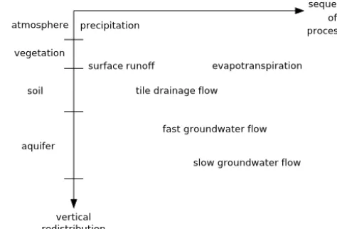
Figure 2. Schema of the timing of processes after a precipitation
event based on the concept of vertical water redistribution.
As reported by Kiesel et al. (2010), the catchment has a high water retention potential. Due to the flat topography (27 to 78 m above mean sea level), the water tables are very high in this region (Kiesel et al., 2010) and a high fraction of the agricultural area is drained (Fohrer et al., 2007). The installed tile drainages contribute to fast runoff and consequently in-crease peak flows, especially in winter (Kiesel et al., 2010). Decreasing tile drainage flow is observed from April and May before tile drainage flow stops during the relatively dry summer months (Kiesel et al., 2009).
Another main characteristic of the Kielstau catchment is the close interaction between river and groundwater, which is due to high groundwater water tables that are directly con-nected to the river (Schmalz et al., 2008). The near-surface groundwater is controlled by precipitation, especially in win-ter (Schmalz et al., 2008). A more detailed description of the catchment can be found in Fohrer and Schmalz (2012).
3.2 Hypotheses derived from observed processes The processes observed in the catchment are used in combi-nation with the concept of vertical water redistribution (Yil-maz et al., 2008) to derive hypotheses about the temporal se-quence of observed processes (Table 1). The vertical redistri-bution of water between faster and slower runoff components after excess rainfall is one of the primary functions of the wa-tershed system (Yilmaz et al., 2008). Accordingly, we distin-guish between the different processes of surface runoff, tile drainage flow, fast (primary) and slow (secondary) ground-water flow and evapotranspiration (Fig. 3).
Based on the findings of Kiesel et al. (2010) for the study catchment and Fig. 2, it is hypothesised that the magnitude and timing of surface runoff is relevant during the whole year whenever the amount of precipitation exceeds the soil infil-tration capacity (H1: surface runoff upon rainfall).
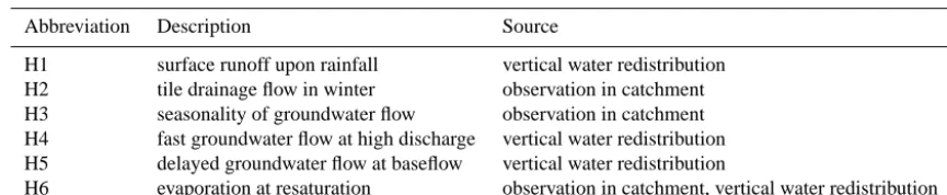
Table 1. Hypotheses for model verification, derived from theory of vertical water redistribution and hydrological processes observed within
the catchment.
Abbreviation Description Source
H1 surface runoff upon rainfall vertical water redistribution
H2 tile drainage flow in winter observation in catchment
H3 seasonality of groundwater flow observation in catchment
H4 fast groundwater flow at high discharge vertical water redistribution
H5 delayed groundwater flow at baseflow vertical water redistribution
H6 evaporation at resaturation observation in catchment, vertical water redistribution
2001 2002 2003 2004
0.0 0.2 0. 4 0. 6 0.8 1.0
a) surface runoff
se ns iti vi ty CN2 SURLAG
2001 2002 2003 2004
0.0 0.2 0. 4 0. 6 0.8 1.0 se ns iti vi ty
b) tile drainage flow
GDRAIN LATKSATF
2001 2002 2003 2004
0.0 0.2 0. 4 0. 6 0.8 1.0 se ns iti vi ty
c) fast shallow aquifer
RCHRGssh ALPHA_BFfsh
2001 2002 2003 2004
0.0 0.2 0. 4 0. 6 0.8 1.0 se ns iti vi ty
d) slow shallow aquifer
RCHRGdp ALPHA_BFssh
2001 2002 2003 2004
0.0 0.2 0. 4 0. 6 0.8 1.0
e) evaporation and soil water storage
se ns iti vi ty SOL_AWC ESCO
2001 2002 2003 2004
0 1 2 3 4 5 6 di sc ha rg e [m ³/s ] 200 15 0 100 50 0 pr ec ip ita tio n [m m ] SDRAIN GW_DELAYfsh GW_DELAYssh
Figure 3. Temporal parameter sensitivities for all analysed model
parameters from 2001 to 2004. Based on the processes they con-trol, the parameters are grouped into surface runoff (a), tile drainage flow (b), process dynamics of the fast shallow aquifer (c) and the slow shallow aquifer (d), evaporation, and soil water storage (e). The bottom plot shows the observed discharge and precipitation.
depending on the soil water storage capacity. As shown by Kiesel et al. (2009, 2010) and Schmalz et al. (2008), the stor-age capacity in the catchment is directly connected with tile drainage and groundwater dynamics. In winter, groundwater tables are high, which results in a high potential for ground-water extraction through the tile drainages (Kiesel et al., 2010). Based on the observations of Kiesel et al. (2009), tile drainage flow is expected to cause peak flows in winter due to groundwater ponding and a high soil water content. Con-sequently, we hypothesise that the tile drainage flow is highly relevant in winter and of minor importance in summer (H2: tile drainage flow in winter).
High groundwater tables are one of the most important hydrological characteristics in the study catchment. During winter periods, the groundwater dynamics are mainly trolled by precipitation inputs due to a direct hydraulic con-nection between groundwater and the river (Schmalz et al., 2008). In summer, the extent of groundwater–surface water interactions decreases, but groundwater storage remains the main contributor of flow to the river (Schmalz et al., 2008). Based on these assumptions, we hypothesise a high relevance of fast groundwater flow in winter and high relevance of the slow groundwater flow in the beginning of summer (H3: sea-sonality of groundwater flow).
More specifically, recharge from the quickly reacting aquifer is high during high discharge periods in winter. This fast groundwater recharge leads to increasing dominance of the outflow from this aquifer at decreasing high discharge (H4: fast groundwater flow at high discharge). At the begin-ning of the recession, the delayed recharge is expected to be the main process controlling the discharge generation (H5: slow groundwater contribution at baseflow).
compensa-tion in dry summer months until the beginning of resaturacompensa-tion phases in autumn (H6: evaporation at resaturation).
3.3 TEDPAS application
TEDPAS was applied to a hydrological model to obtain tem-poral parameter sensitivities, which are used to derive infor-mation about the timing of specific hydrological processes. Based on this, a temporal sequence of simulated processes is derived. In the following, the hydrological model and the application of TEDPAS is described in detail.
3.3.1 Model description and setup
In our study, TEDPAS was applied to the semi-distributed, ecohydrological SWAT model (Arnold et al., 1998). The SWAT model uses distinct spatial positions for the subbasins within the catchment. Within the subbasins, Hydrological Response Units (HRU) are used to describe areas of the same land use, slope and soil. The different components of the SWAT model have an empirical and process-oriented char-acter. Due to the incorporation of several model components, there is a high number of parameters, which strongly in-creases the complexity of the SWAT model (Cibin et al., 2010).
The water balance is driven mainly by the processes of pre-cipitation, evapotranspiration, runoff, soil water percolation, drainage and groundwater flow. Runoff is routed through the main reaches of the subbasins to the catchment outlet. A de-tailed description of process implementation and the theory about the SWAT model can be found in Neitsch et al. (2011). Catchment-specific input data are required to set up the model, including a soil map (resolution 1 : 200 000, BGR, 1999) and a digital elevation model (resolution 5 m; LVermA, 1995). The data on land use and crop rotations used in this study were derived from two mapping campaigns during the cropping seasons 2011/2012 and 2012/2013 (Pfannerstill et al., 2014a, b). The spatial distribution of tile drainages and databases for soil and crops were obtained from Fohrer et al. (2013, 2007).
Precipitation data were provided by the Gluecksburg– Meierwik weather station located north of the Kielstau catch-ment (DWD, 2012). Additional weather input that is based on regional interpolation (Oesterle, 2001) was used to fill gaps of data that are needed. In this study, interpolated data of wind speed, temperature, solar radiation, and humidity were used to fill data gaps.
During model setup, 36 subbasins and 2214 HRUs, which were determined using three slope classes (<2.6, 2.6–4.6 and>4.6 %), were defined with the ArcSWAT interface (ver-sion 2012.10.1.6). For the application of the TEDPAS-based model verification, the SWAT3S version (Pfannerstill et al.,
2014a) with its modified groundwater structure was used. Therefore, the groundwater input files were reprocessed us-ing a script in the R environment (R Core Team, 2013) to
add the additional groundwater input parameters required by SWAT3S.
3.3.2 Model simulations
Model simulations were carried out to obtain a basis for the analysis with TEDPAS. To achieve equilibrium for the dif-ferent storages of the model, a warm-up period from 1997 to 2000 was chosen. The temporal sensitivity analysis was performed for the hydrological years of 2001 to 2004. TED-PAS provided the dynamics of temporal parameter sensitiv-ity for the analysed model. The model parameters (Table 2) and their ranges were selected according to previous SWAT model studies (Pfannerstill et al., 2014a; Guse et al., 2014, 2015). Based on the parameter variation set that was gen-erated with FAST (Reusser, 2012), TEDPAS required 687 model runs.
After performing all model runs, TEDPAS provides a tem-poral sequence of simulated processes that is based on the parameter sensitivity. The sensitivity of parameters was as-signed to the processes of surface runoff, tile drainage flow, groundwater flow, evaporation, and soil water storage. These simulated processes and its interpretation to a temporal se-quence of simulated processes are the core results of TED-PAS for the model verification.
3.4 Process verification of SWAT3S with
TEDPAScatchment
The agreement between the temporal sequences of observed and simulated processes is determined by comparing both se-quences with each other. The temporal sequence of processes observed in the study catchment is described with hypotheses that were formulated based on information about the hydro-logical processes occurring in the catchment. The temporal model parameter sensitivities that are provided by TEDPAS are used to analyse the timing of hydrological processes and to identify the temporal sequence of simulated processes. Fi-nally, both temporal sequences are compared to verify the model results with respect to processes observed in the study catchment.
4 Description and discussion of the results
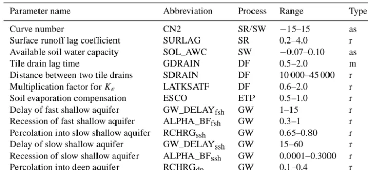
Table 2. Selection of parameters and their ranges for the temporal sensitivity analyses. The three methods to change parameter values used
are replacement (r), multiplication (m), and addition/subtraction (as). The parameters are assigned to the hydrological process they control including surface runoff (SR), soil water storage (SW), drainage flow (DF), evapotranspiration (ETP), and groundwater flow (GW)
Parameter name Abbreviation Process Range Type
Curve number CN2 SR/SW −15–15 as
Surface runoff lag coefficient SURLAG SR 0.2–4.0 r
Available soil water capacity SOL_AWC SW −0.07–0.10 as
Tile drain lag time GDRAIN DF 0.5–2.0 m
Distance between two tile drains SDRAIN DF 10 000–45 000 r
Multiplication factor forKe LATKSATF DF 0.6–2.0 r
Soil evaporation compensation ESCO ETP 0.5–1.0 r
Delay of fast shallow aquifer GW_DELAYfsh GW 1–15 r
Recession of fast shallow aquifer ALPHA_BFfsh GW 0.3–1 r
Percolation into slow shallow aquifer RCHRGssh GW 0.65–0.80 r
Delay of slow shallow aquifer GW_DELAYssh GW 15–60 r
Recession of slow shallow aquifer ALPHA_BFssh GW 0.0001–0.3000 r
Percolation into deep aquifer RCHRGdp GW 0.1–0.4 r
the derived hypotheses against the temporal parameter sensi-tivity (Fig. 4).
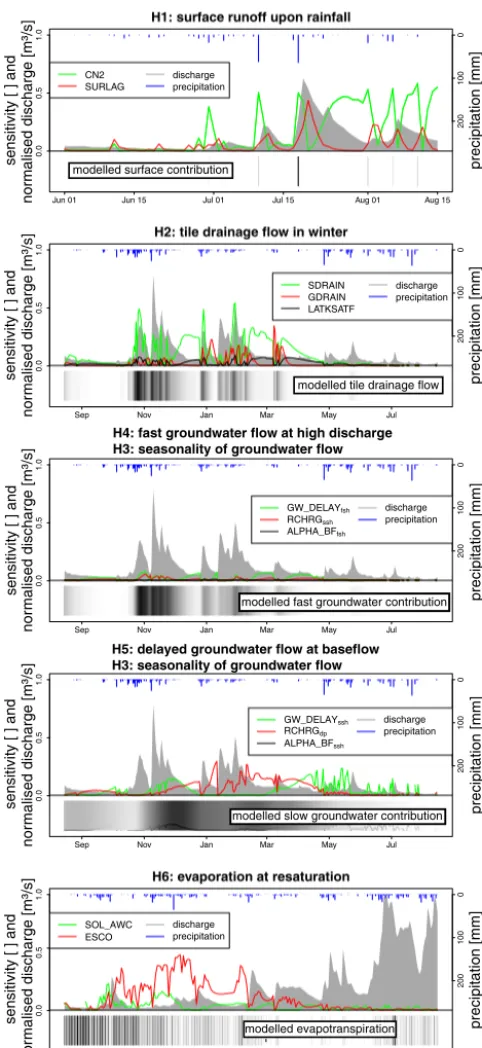
The impact of the model parameters controlling surface runoff (SURLAG and CN2) was observed during discharge peaks throughout the year (Fig. 4). The model component for simulated surface runoff is the first component to be-come sensitive during a rainfall event, which confirms hy-pothesis H1. The temporal sequence of observed processes in the study catchment, which was based on the observations of Kiesel et al. (2010), is confirmed by the sensitivity of the two parameters, which is clearly linked to short peak flow events and single surface runoff events (Figs. 3 and 4). Ad-ditionally, it is clearly shown that these events are connected to high amounts of daily precipitation.
All other parameters showed a characteristic temporal pa-rameter sensitivity, which depends on the discharge mag-nitude and the moisture conditions. The impact of tile drainages (GDRAIN, SDRAIN, and LATKSATF) was very low in phases of low discharge during summer and espe-cially high in winter (Fig. 4). This finding verifies hypotheses H1 and H2: tile drainages are inactive when groundwater ta-bles, which do not rise during the short and low precipitation events in summer periods, are low. The most pronounced dy-namic of sensitivity and influence on the discharge was ob-served during wet periods in winter and spring (Fig. 4), when rising water tables are expected due to sufficient precipita-tion.
The low impact of the tile drainages during low flow peri-ods can be further explained by the groundwater dominance, which is the next step in the temporal sequence of observed processes that is described by the concept of vertical water redistribution (see Fig. 2). The high impact of groundwater on discharge for the studied lowland catchment is particu-larly visible at the beginning and the end of the long-lasting low flow periods, which confirms hypothesis H3.
Additionally, there is a clear separation for the relevance of the fast and the slow shallow aquifers. The time delay for recharge of the fast shallow aquifer (GW_DELAYfsh) becomes less relevant when the influence of the time delay parameter of the slow shallow aquifer (GW_DELAYssh) in-creases. This result clearly depicts the fast shallow aquifer recharge at high discharge with fast groundwater contribu-tion (ALPHA_BFfsh), followed by a delayed slow shallow aquifer recharge at recession phases with slow groundwa-ter contribution (ALPHA_BFfsh, H3, H4, H5). Consequently, the low flow during dry periods is controlled by flow from the slow shallow aquifer to the channel (Fig. 4). This finding supports hypothesis H3, which expects a high relevance of the slow shallow aquifer parameters in the beginning of the low flow period in summer but low relevance in winter.
In general, the fast shallow aquifer had very limited impact on the discharge, because the tile drainage flow controls the water amount recharging the groundwater. Consequently, the process of fast discharge generation in winter is controlled by both the tile drainage flow and the fast shallow aquifer (Fig. 4). This was partly expected, since the parameters of the fast shallow aquifer were hypothesised to be mainly relevant in winter (H4). Due to the low parameter sensitivity of the fast shallow aquifer, hypothesis H4 is partly verified. How-ever, the modelled discharge contribution of tile drainages and the fast shallow aquifer indicates simultaneous activity of both hydrological processes.
avail-CN2 SURLAG
discharge precipitation
Jun 01 Jun 15 Jul 01 Jul 15 Aug 01 Aug 15 H1: surface runoff upon rainfall
0.0
0.5
1.0
modelled surface contribution
200 100 0 precip itation [mm] normal ised discha rge [ m³/s]
Sep Nov Jan Mar May Jul
H2: tile drainage flow in winter
0.0 0.5 1.0 200 100 0 precip itation [mm] nor mal ised discha rge [ m³/s] SDRAIN GDRAIN LATKSATF discharge precipitation
Sep Nov Jan Mar May Jul
H4: fast groundwater flow at high discharge
H3: seasonality of groundwater flow w
0.0 0.5 1.0 200 100 0 precip itation [mm] nor mal ised discha rge [ m³/s] GW_DELAYfsh RCHRGssh ALPHA_BFfsh discharge precipitation
Sep Nov Jan Mar May Jul
H5: delayed groundwater flow at baseflow
H3: seasonality of groundwater flow w
0.0 0.5 1.0 200 100 0 precip itation [mm] s nor mal ised discha rge [ m³/s] GW_DELAYssh RCHRGdp ALPHA_BFssh discharge precipitation
Sep Nov Jan Mar
H6: evaporation at resaturation
0.0 0.5 1.0 SOL_AWC ESCO discharge precipitation 200 100 0 precip itation [mm] nor mal ised discha rge [ m³/s] sen sitivi ty [ ] and sen sitivi ty [ ] and sen sitivi ty [ ] and sen sitivi ty [ ] and sen sitivi ty [ ] and
modelled tile drainage flow
modelled fast groundwater contribution
modelled slow groundwater contribution
[image:8.612.46.287.85.609.2]modelled evapotranspiration
Figure 4. Periods of temporal parameter sensitivities for the
veri-fication of hypotheses about surface runoff (H1), tile drainage flow (H2), the process dynamics of the fast shallow aquifer (H3, H4) and the slow shallow aquifer (H3, H5), evaporation, and soil water stor-age (H6). The normalised observed discharge and the precipitation are shown for each subplot. Additionally, the modelled hydrological output is averaged and normalised to show the range between low (white) and high (black) intensity.
able for the slow shallow and the inactive deep aquifer. This behaviour is consistent with the observed processes of the study catchment as the recharge to the fast shallow aquifer is intended to be more important during wet phases with fast groundwater recharge (H3, H4). In contrast, the slow shallow aquifer controls the slow recharge before recession phases (H3, H5).
The processes expected to become relevant last accord-ing to the concept of vertical water redistribution (Fig. 2) are the storage function of the soils and evaporation. The evap-oration and soil water availability parameters (ESCO and SOL_AWC) are most relevant during low flow periods in late summer and during phases of resaturation in the beginning of autumn (Figs. 3 and 4). During these periods, the influ-ence of all other processes is very limited. This highlights the relevance of additional storages besides the aquifers for the generation of baseflow in dry periods. Since the parame-ter sensitivities of the groundwaparame-ter component are very low in these periods, hypothesis H6 is verified (Fig. 4).
The verified temporal sequence of processes proves the hydrological consistency of the simulated processes. How-ever, additional information about the model’s behaviour may be used to support this finding. For this, we refer to previous studies of Pfannerstill et al. (2014b). In these stud-ies, Pfannerstill et al. (2014b) clearly showed the ability of SWAT3Sto reproduce the daily discharge for the study
catch-ment. With respect to timing and dynamics, SWAT3Sshowed
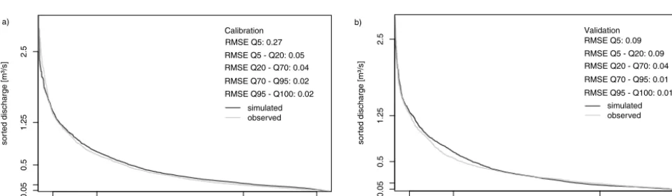
satisfactory model performance for the calibration and vali-dation periods (Fig. 5). In addition, Pfannerstill et al. (2014b) validated the reproduction of discharge magnitudes for the validation and calibration periods by extracting information about the ability of SWAT3S to realistically simulate
hydro-logic characteristics for the study catchment (Fig. 6a and b). In combination with the results of Pfannerstill et al. (2014b), the findings of this study confirm that SWAT3S is
able to simulate the investigated hydrological processes ad-equately. This evidence is provided by satisfying model per-formance in simulating daily discharge dynamics and mag-nitudes and the appropriate simulation of process dynamics.
5 Relevance of TEDPAS for model verifications
TEDPAS is a central method for model diagnostics and the verification of models (Fig. 1). We developed TEDPAScatchment, which is a verification framework that uses processes observed in a catchment in combination with TED-PAS. In the following, it is discussed if the presented verifi-cation framework provides useful diagnostic information for the verification of hydrological models.
2000 2002 2004 2006 2008 2010
0
1
2
3
4
discharge [m³/s]
simulated observed
calibration validation calibration validation
Performance for:
calibration
validation NSE: PBIAS:
NSE: PBIAS:
0.72 4.4
[image:9.612.54.539.65.240.2]0.67 -5.4
Figure 5. Daily observed (grey) and simulated (black) discharge for the study catchment with model performance (Nash–Sutcliffe efficiency
(NSE) and percent bias (PBIAS)) for the calibration and validation period after Pfannerstill et al. (2014b).
white
Q5 Q20 Q70 Q95
0.05
0.5
1.25
2.5
sor
ted disch
arge [m³/s]
simulated observed Calibration RMSE Q5: 0.27 RMSE Q5 - Q20: 0.05 RMSE Q20 - Q70: 0.04 RMSE Q70 - Q95: 0.02 RMSE Q95 - Q100: 0.02
white
Q5 Q20 Q70 Q95
0.05
0.5
1.
25
2.5
sor
ted disch
arge [m³/s]
simulated observed Validation RMSE Q5: 0.09 RMSE Q5 - Q20: 0.09
RMSE Q95 - Q100: 0.01 RMSE Q20 - Q70: 0.04 RMSE Q70 - Q95: 0.01
a) b)
Figure 6. Flow duration curve of observed (grey) and simulated (black) discharge magnitudes for the calibration period (a) and the validation
period (b). The model performance is depicted with root-mean-square error (RMSE) of the different flow duration curve segments according to Pfannerstill et al. (2014b).
more general context. We hypothesise that TEDPAScatchment is applicable to any hydrological model in any catchment.
Our analysis of model results showed that there is the ne-cessity to analyse the relevance of individual model parame-ters. In our study, we focused on hydrological processes that are identifiable at daily resolution, which facilitated the de-tection of the groundwater processes of the model (fast- and slow-reacting aquifer). Despite a clear separation of the two groundwater storages, the verification of dynamics for the fast aquifer was limited due to low parameter sensitivity of the fast groundwater model component. Nevertheless, all hy-pothesised processes were part of the temporal sequence of simulated processes. The case study results revealed a tem-poral sequence of simulated processes that is consistent with the processes observed in the study catchment and the con-cept of vertical water redistribution (Fig. 2). The temporal sequence of simulated processes exhibited the order with sur-face runoff as the first process, followed by tile drainage flow. Finally, this temporal sequence continues with fast
ground-water flow and slow groundground-water flow (Figs. 3 and 4). How-ever, the low sensitivity of the parameters to the fast shallow aquifer limits the verification to a certain extent. Nonethe-less, the temporal sequence of processes is identifiable. Con-sequently, the confirmation of the hydrological consistency is the core result of the diagnostic analysis. It indicates that the simplified process representation is in accordance with the concept of vertical process dynamics.
[image:9.612.59.541.284.425.2]In this study, TEDPAScatchment was applied using com-monly available, daily observed discharge data. The high temporal resolution facilitated the diagnosis of the model structure and its ability to simulate the processes that were observed in the catchment. Thereby, TEDPAS provided additional diagnostic information to understand the repre-sentation of processes within the analysed model. Addi-tionally, the presented example highlights the potential of TEDPAScatchmentto evaluate the consistency of parameters and process structure using qualitative data. We used pro-cesses observed in the catchment, as well as the concept of vertical water redistribution (Fig. 2) to derive hypotheses for the model verification. Additional measured data would al-low a more detailed quantitative evaluation but it has to be kept in mind that this kind of data is generally not available for large catchments.
Regardless of the kind and amount of available data, this study shows that TEDPAS is needed for the extraction of comprehensive model diagnostic information. The applica-tion of TEDPAS in our demonstraapplica-tion example revealed that the highest sensitivity of multiple parameters of different hy-drological processes may occur simultaneously. This find-ing emphasises the importance of TEDPAS, which can be also used to identify the overlapping dominance of different model components and the corresponding hydrological pro-cesses.
6 Conclusions
The main capability of model diagnostics is the determi-nation of the adequacy of process descriptions in model structures. In this study, we used TEDPAS as a verification method in model diagnostics. As shown in Fig. 1, we propose five aspects that need to be considered for model diagnostics and the verification of models.
The proposed framework for model verification requires (i) observations and knowledge about the catchment to (ii) derive hypotheses about the temporal sequence of ob-served processes. Contrary to processes obob-served in the catchment, TEDPAS is used to (iii) calculate temporal pa-rameter sensitivities to (iv) extract the temporal sequence of simulated processes. Finally, the model verification is per-formed by (v) determining the agreement between the se-quences of observed and simulated processes.
Based on our results, we propose TEDPAS as a method to provide relevant diagnostic information. TEDPAS is applied to analyse the temporal sequence of processes of all relevant hydrological processes.
The main outcomes of this study are as follows:
– TEDPAScatchment provides diagnostic information for the verification of the consistency between the tem-poral sequence of observed and simulated processes. The temporal sequence of observed processes is derived
from qualitative knowledge of the catchment, and the concept of vertical water redistribution.
– TEDPAS provides the temporal sequence of simulated processes for comparison against the temporal sequence of observed processes.
We recommend the use of TEDPAScatchmentas a verifica-tion framework for model diagnostics since it provides rele-vant information, which leads to an improved understanding of the relationship between model structure and the processes occurring in a catchment.
Acknowledgements. The Government-Owned Company for
Coastal Protection, National Parks and Ocean Protection, provided the discharge data for this study. The digital elevation model and the river net were obtained from the land survey office of Schleswig-Holstein. We thank the German Weather Service (DWD) for providing the climate data and the Potsdam Institute for Climate Impact Research (PIK) for providing the STAR data.
Many thanks to Katrin Bieger (Blackland Research & Exten-sion Center, Texas A&M AgriLife) for the proofreading of various manuscript versions. We are thankful to the Erwin Zehe, Shervan Gharari, and the anonymous reviewer for their insightful comments. The paper greatly benefitted from their comments.
Matthias Pfannerstill was supported by a scholarship of the Ger-man Environmental Foundation (DBU). The DFG-funded project GU 1466/1-1 (hydrological consistency in modelling) supported the work of Bjön Guse. Dominik Reusser was supported by the BMBF via its initiative Potsdam Research Cluster for Georisk Analysis, Environmental Change and Sustainability (PROGRESS – grant: 03IS2191B). We want to thank the community of the open-source software R, which was used for the calibration of the SWAT model and following analysis.
Edited by: E. Zehe
References
Arnold, J. G., Srinivasan, R., Muttiah, R. S., and Williams, J. R.: Large area hydrologic modeling and assessment part I: Mmodel development, J. Am. Water Resour. As., 1, 73–89, doi:10.1111/j.1752-1688.1998.tb05961.x, 1998.
BGR: Bundesanstalt fuer Geowisschenschaften und Rohstoffe – Bodenuebersichtskarte im Maßstab 1 : 200.000, Verbreitung der Bodengesellschaften, 1999.
Boyle, D. P., Gupta, H. V., and Sorooshian, S.: Toward improved calibration of hydrologic models: Combining the strengths of manual and automatic methods, Water. Resour. Res., 36, 3663– 3674, doi:10.1029/2000wr900207, 2000.
Boyle, D. P., Gupta, H. V., Sorooshian, S., Koren, V., Zhang, Z., and Smith, M.: Toward improved streamflow forecasts: Value of semidistributed modeling, Water. Resour. Res., 37, 2749–2759, doi:10.1029/2000WR000207, 2001.
Clark, M. P., McMillan, H. K., Collins, D. B. G., Kavetski, D., and Woods, R. A.: Hydrological field data from a modeller’s perspec-tive: Part 2: process-based evaluation of model hypotheses, Hy-drol. Process., 25, 523–543, doi:10.1002/hyp.7902, 2011. Cloke, H., Pappenberger, F., and Renaud, J.-P.: Multi-method
global sensitivity analysis (MMGSA) for modelling flood-plain hydrological processes, Hydrol. Process., 22, 1660–1674, doi:10.1002/hyp.6734, 2008.
Cukier, R. I., Fortuin, C. M., Shuler, K. E., Petschek, A. G., and Schaibly, J. H.: Study of sensitivity of coupled reaction systems to uncertainties in rate coefficients. 1. Theory, J. Chem. Phys., 59, 3873–3878, doi:10.1063/1.1680571, 1973.
Cukier, R. I., Schaibly, J. H., and Shuler, K. E.: Study of sensitivity of coupled reaction systems to uncertainties in rate coefficients. 3. Analysis of approximations, J. Chem. Phys., 63, 1140–1149, doi:10.1063/1.431440, 1975.
Cukier, R. I., Levine, H. B., and Shuler, K. E.: Non-linear sensitivity analysis of multi-parameter model systems, J. Comput. Phys., 26, 1–42, doi:10.1016/0021-9991(78)90097-9, 1978.
DWD: Weather and climate data from the German Weather Ser-vice (DWD) of the station Flensburg (1961–1990), Online cli-mate data, 2012.
Euser, T., Winsemius, H. C., Hrachowitz, M., Fenicia, F., Uhlen-brook, S., and Savenije, H. H. G.: A framework to assess the realism of model structures using hydrological signatures, Hy-drol. Earth Syst. Sci., 17, 1893–1912, doi:10.5194/hess-17-1893-2013, 2013.
Fenicia, F., Savenije, H., and Winsemius, H.: Moving from model calibration towards process understanding, Phys. Chem. Earth, 33, 1057–1060, doi:10.1016/j.pce.2008.06.008, 2008.
Fohrer, N. and Schmalz, B.: Das UNESCO
Oekohydrologie-Referenzprojekt Kielstau-Einzugsgebiet – Nachhaltiges
Wasserressourcenmanagement und Ausbildung im
laendlichen Raum, Hydrol. Wasserbewirts., 4, 160–168,
doi:10.5675/HyWa_2012,4_1, 2012.
Fohrer, N., Schmalz, B., Tavares, F., and Golon, J.: Modelling the landscape water balance of mesoscale lowland catchments con-sidering agricultural drainage systems, Hydrol. Wasserbewirts., 51, 164–169, 2007.
Fohrer, N., Dietrich, A., Kolychalow, O., and Ulrich, U.: Assess-ment of the EnvironAssess-mental Fate of the Herbicides Flufenacet and Metazachlor with the SWAT Model, J. Environ. Qual., 42, 1–11, doi:10.2134/jeq2011.0382, 2013.
Garambois, P. A., Roux, H., Larnier, K., Castaings, W., and Dar-tus, D.: Characterization of process-oriented hydrologic model behavior with temporal sensitivity analysis for flash floods in Mediterranean catchments, Hydrol. Earth Syst. Sci., 17, 2305– 2322, doi:10.5194/hess-17-2305-2013, 2013.
Gupta, H. V., Wagener, T., and Liu, Y.: Reconciling theory with observations: Elements of a diagnostic approach to model eva-lution, Hydrol. Process., 22, 3802–3813, doi:10.1002/hyp.6989, 2008.
Gupta, H. V., Clark, M. P., Vrugt, J. A., Abramowitz, G., and Ye, M.: Towards a comprehensive assessment of model structural adequacy, Water Resour. Res., 48, W08301, doi:10.1029/2011WR011044, 2014.
Guse, B., Reusser, D. E., and Fohrer, N.: How to improve the representation of hydrological processes in SWAT for a low-land catchment – Temporal analysis of parameter
sensitiv-ity and model performance, Hydrol. Process., 28, 2651–2670, doi:10.1002/hyp.9777, 2014.
Guse, B., Pfannerstill, M., and Fohrer, N.: Dynamic modelling of land use change impacts on nitrate loads in rivers, Environ. Pro-cess., 1–18, doi:10.1007/s40710-015-0099-x, 2015.
Haas, M., Guse, B., Pfannerstill, M., and Fohrer, N.: Detection of dominant nitrate processes in ecohydrological modelling with temporal parameter sensitivity analysis, Ecol. Model., 314, 62– 71, doi:10.1016/j.ecolmodel.2015.07.009, 2015.
Herbst, M., Gupta, H. V., and Casper, M. C.: Mapping model be-haviour using Self-Organizing Maps, Hydrol. Earth Syst. Sci., 13, 395–409, doi:10.5194/hess-13-395-2009, 2009.
Herman, J. D., Reed, P. M., and Wagener, T.: Time-varying sen-sitivity analysis clarifies the effects of watershed model formu-lation on model behavior, Water Resour. Res., 49, 1400–1414, doi:10.1002/wrcr.20124, 2013.
Hrachowitz, M., Fovet, O., Ruiz, L., Euser, T., Gharari, S., Nijzink, R., Freer, J., Savenije, H., and Gascuel-Odoux, C.: Process con-sistency in models: The importance of system signatures, ex-pert knowledge, and process complexity, Water Resour. Res., 50, 7445–7469, doi:10.1002/2014wr015484, 2014.
Kiesel, J., Schmalz, B., and Fohrer, N.: SEPAL – a simple GIS-based tool to estimate sediment pathways in lowland catchments, Adv. Geosci., 21, 25–32, doi:10.5194/adgeo-21-25-2009, 2009. Kiesel, J., Fohrer, N., Schmalz, B., and White, M. J.: Incorporating
landscape depressions and tile drainages of a northern German lowland catchment into a semi-distributed model, Hydrol. Pro-cess., 24, 1472–1486, doi:10.1002/hyp.7607, 2010.
Kirchner, J. W.: Getting the right answers for the right rea-sons: Linking measurements, analyses, and models to advance the science of hydrology, Water Resour. Res., 42, W03S04, doi:10.1029/2005WR004362, 2006.
LVermA: Landesvermessungsamt Schleswig-Holstein – Digitales Geländemodell fuer SchleswigHolstein. Quelle: TK25.
Gitter-weite 25 m×25 m und TK50 Gitterweite 50 m×50 m sowie
ATKIS-DGM2-1 m×1 m Gitterweite und DGM 5 m×5 m
Git-terweite, abgeleitet aus LiDAR-Daten, 1995.
Martinez, G. and Gupta, H.: Hydrologic consistency as a ba-sis for assessing complexity of monthly water balance mod-els for the continental United States: Hydrologic consistency and model complexity, Water Resour. Res., 47, W12540, doi:10.1029/2011WR011229, 2011.
Massmann, C., Wagener, T., and Holzmann, H.: A new approach to visualizing time-varying sensitivity indices for environmen-tal model diagnostics across evaluation time-scales, Environ. Model. Softw., 51, 190–194, doi:10.1016/j.envsoft.2013.09.033, 2014.
Neitsch, S. L., Arnold, J. G., Kiniry, J. R., and Williams, J. R.: SWAT Theoretical Documentation Version 2009, Grassland, Soil and Water Research Laboratory, Agricultural Research Service, Blackland Research Center, Texas Agricultural Experiment Sta-tion, 2011.
Nossent, J., Elsen, P., and Bauwens, W.: Sobol’ sensitivity analyses of a complex environmental model, Environ. Model. Softw., 26, 1515–1525, doi:10.1016/j.envsoft.2011.08.010, 2011.
Pfannerstill, M., Guse, B., and Fohrer, N.: A multi-storage ground-water concept for the SWAT model to emphasize nonlinear groundwater dynamics in lowland catchments, Hydrol. Process., 28, 5599–5621, doi:10.1002/hyp.10062, 2014a.
Pfannerstill, M., Guse, B., and Fohrer, N.: Smart low flow sig-nature metrics for an improved overall performance eval-uation of hydrological models, J. Hydrol., 510, 447–458, doi:10.1016/j.jhydrol.2013.12.044, 2014b.
Razavi, S. and Gupta, H. V.: What do we mean by sensitivity anal-ysis? The need for comprehensive characterization of “global” sensitivity in Earth and Environmental systems models, Wa-ter Resour. Res., 51, 3070–3092, doi:10.1002/2014WR016527, 2015.
R Core Team: R: A language and environment for statistical com-puting. Vienna, Austria: R Foundation for Statistical Computing, 2013.
Reusser, D.: Implementation of the Fourier Amplitude Sensitivity Test (FAST), R-package, 0.61, 2012.
Reusser, D. E. and Zehe, E.: Inferring model structural deficits by analyzing temporal dynamics of model performance and parameter sensitivity, Water Resour. Res., 47, W07550, doi:10.1029/2010WR009946, 2011.
Reusser, D. E., Blume, T., Schaefli, B., and Zehe, E.: Analysing the temporal dynamics of model performance for hydrological mod-els, Hydrol. Earth Syst. Sci., 13, 999–1018, doi:10.5194/hess-13-999-2009, 2009.
Reusser, D. E., Buytaert, W., and Zehe, E.: Temporal dynamics of model parameter sensitivity for computationally expensive mod-els with FAST (Fourier Amplitude Sensitivity Test), Water Re-sour. Res., 47, W07551, doi:10.1029/2010WR009947, 2011. Saltelli, A. and Bolado, R.: An alternative way to compute Fourier
amplitude sensitivity test (FAST), Comput. Stat. Data Anal., 26, 445–460, doi:10.1016/S0167-9473(97)00043-1, 1998.
Saltelli, A., Ratto, M., Tarantola, S., and Campolongo,
F.: Sensitivity analysis practices: Strategies for
model-based inference, Reliab. Eng. Syst. Safe., 91, 1109–1125, doi:10.1016/j.ress.2005.11.014, 2006.
Schmalz, B., Springer, P., and Fohrer, N.: Interactions between near-surface groundwater and near-surface water in a drained riparian wet-land, in: Proceedings of International Union of Geodesy and Geophysics XXIV General Assemble “A New Focus on Inte-grated Analysis of Groundwater/Surface Water Systems”, Peru-gia, Italy, 11–13 July 2007, 21–29, IAHS Press, 2008.
Sieber, A. and Uhlenbrook, S.: Sensitivity analyses of a distributed catchment model to verify the model structure, J. Hydrol., 310, 216–235, doi:10.1016/j.jhydrol.2005.01.004, 2005.
Sudheer, K. P., Lakshmi, G., and Chaubey, I.: Application of a pseudo simulator to evaluate the sensitivity of parameters in com-plex watershed models, Environ. Model. Softw., 26, 135–143, doi:10.1016/j.envsoft.2010.07.007, 2011.
van Griensven, A., Meixner, T., Grundwald, S., Bishop, T., Diluzio, M., and Srinivasan, R.: A global sensitivity analysis tool for the parameters of multi-variable catchment models, J. Hydrol., 324, 10–23, doi:10.1016/j.jhydrol.2005.09.008, 2006.
van Werkhoven, K., Wagener, T., Reed, P., and Tang, Y.: Sensitivity-guided reduction of parametric dimensionality for multi-objective calibration of watershed models, Adv. Water Resour., 32, 1154–1169, doi:10.1016/j.advwatres.2009.03.002, 2009.
Wagener, T., Boyle, D. P., Lees, M. J., Wheater, H. S., Gupta, H. V., and Sorooshian, S.: A framework for development and applica-tion of hydrological models, Hydrol. Earth Syst. Sci., 5, 13–26, doi:10.5194/hess-5-13-2001, 2001.
Wagener, T., McIntyre, N., Lees, M., Wheater, H., and Gupta, H.: Towards reduced uncertainty in conceptual rainfall-runoff mod-elling: Dynamic identifiability analysis, Hydrol. Process., 17, 455–476, doi:10.1002/hyp.1135, 2003.
Wagener, T., Reed, P., van Werkhoven, K., Tang, Y., and Zhang, Z.: Advances in the identification and evaluation of com-plex environmental systems models, J. Hydroinform., 11, 266, doi:10.2166/hydro.2009.040, 2009.