temperature and surface energy balance using MODIS and SEBS
F. Alkhaier1, Z. Su1, and G. N. Flerchinger2
1Department of Water Resources, Faculty of Geo-Information Science and Earth Observation, University of Twente,
Enschede, The Netherlands
2Northwest Watershed Research Center, United States Department of Agriculture, Washington, D.C., USA
Correspondence to: F. Alkhaier ([email protected])
Received: 7 September 2011 – Published in Hydrol. Earth Syst. Sci. Discuss.: 23 September 2011 Revised: 5 June 2012 – Accepted: 8 June 2012 – Published: 3 July 2012
Abstract. The possibility of observing shallow groundwater depth and areal extent using satellite measurements can sup-port groundwater models and vast irrigation systems man-agement. Moreover, these measurements can help to include the effect of shallow groundwater on surface energy bal-ance within land surface models and climate studies, which broadens the methods that yield more reliable and informa-tive results. To examine the capacity of MODIS in detect-ing the effect of shallow groundwater on land surface tem-perature and the surface energy balance in an area within Al-Balikh River basin in northern Syria, we studied the in-terrelationship between in-situ measured water table depths and land surface temperatures measured by MODIS. We, also, used the Surface Energy Balance System (SEBS) to cal-culate surface energy fluxes, evaporative fraction and daily evaporation, and inspected their relationships with water ta-ble depths. We found out that the daytime temperature in-creased while the nighttime temperature dein-creased when the depth of the water table increased. And, when the water table depth increased, net radiation, latent and ground heat fluxes, evaporative fraction and daily evaporation decreased, while sensible heat flux increased. This concords with the findings of a companion paper (Alkhaier et al., 2012). The observed clear relationships were the result of meeting both condi-tions that were concluded in the companion paper, i.e. high potential evaporation and big contrast in day-night tempera-ture. Moreover, the prevailing conditions in this study area helped SEBS to yield accurate estimates. Under bare soil conditions and under the prevailing weather conditions, we conclude that MODIS is suitable for detecting the effect of shallow groundwater because it has proper imaging times
and adequate sensor accuracy; nevertheless, its coarse spa-tial resolution is disadvantageous.
1 Introduction
Not only do shallow water table conditions characterize low lands in many drainage basins (Freeze and Cherry, 1979), but it has also become a general feature in many of the world’s large-scale irrigation systems in various countries, i.e. USA, Mexico, China, India, Pakistan, Australia, etc. (Dregne et al., 1996; Rahman, 2008; Umali, 1993; Middleton and Thomas, 1997; Wichelns, 1999; World Bank, 1992; Xiong et al., 1996). The presence of a shallow water table is common in such areas due to high recharge rates, low drainage rates or small topographic slopes (Northey et al., 2006; Wichelns, 1999).
The possibility of utilizing thermal measurements of oper-ational satellites in observing the depth and the areal extent of shallow groundwater can be of great value in their con-tribution to groundwater flow models and in improving the management of vast irrigation systems. Besides, these mea-surements can be useful in observing the effect of shallow groundwater on surface energy balance, and in conveying that effect into land surface models and climate studies on more solid basis.
This early work was followed by the investigation of My-ers and Moore (1972) which made use of seasonal flights with thermal radiometers flown over the Sioux Basin in east-ern South Dakota. Soil temperature data (8.0 to 14.0 µm) were obtained from predawn missions flown on 7 May, 21 July, 26 August and 12 October 1971. The 26 August imagery showed a broad cool area within the flood plain. This cool area extended over farms with a diversity of land use. Furthermore, a high correlation was found between soil temperature and the aquifer thickness. Their study concluded that late August or early September was the best period for thermal detection of shallow aquifers.
Studies which investigated the effect of shallow ground-water on land surface temperature stopped after the early 1980’s (Becker, 2006; Meijerink et al., 2007). Actually, the latest study we could trace back in the literature was the study of Heilman and Moore (1982).
In this study, they correlated radiometric temperatures (10.5 to 12.5 µm) from five scenes captured between 5 June and 4 September 1978 by the Heat Capacity Mapping Mis-sion, with water table depths measured on these dates. Af-ter empirical correction for the vegetation effect, they found that the daytime thermal scene of 4 September had the best correlation. They demonstrated that radiometric temperature measurements from satellites can be correlated with depth to shallow groundwater if proper deliberations were given to the effect of vegetation. Furthermore, they suggested, simi-lar to Huntley (1978), developing a procedure to distinguish groundwater influence from that of soil moisture.
For a more comprehensive view, it is worth mentioning here that some remote sensing studies utilized the thermal effect of shallow water table on snow cover. Some investi-gations focused on this thermal effect on snow when it ac-cumulates and later when it melts over lowlands in relation to the surrounding highlands within a watershed (Falconer et al., 1981). Other investigations focused on how this ef-fect reduces the reflectance and emissivity of the snow cover (Bobba et al., 1992). As long as the target of these studies was the snow cover, the visible to near infrared imageries can be considered more informative than the thermal infrared ones. Despite the humble facilities of earth observation technol-ogy during that early period, keen investigations were con-ducted with regards to tracing the shallow groundwater ef-fect on land surface temperature. It is quite odd how with the availability of satellites orbiting the earth and continu-ously collecting data about the planet surface (Bosilovich et al., 2008), there is hardly any study that has researched the utilization of this reservoir of data in shallow groundwater studies. Furthermore, this data has not been effectively uti-lized in mapping the shallow groundwater effect on land sur-face temperature and sursur-face energy balance components so far.
In a companion paper (Alkhaier et al., 2012), we pre-sented a detailed description of how shallow groundwater affects surface soil moisture, surface soil temperature and
the various components of surface energy balance. We also discussed the optimum conditions under which this effect can be sufficiently clear to be detected by dint of satellite measurements.
In this paper, we aim at inspecting the capacity of MODIS (Moderate-resolution Imaging Spectroradiometer) to detect the effect of shallow groundwater on surface temperature of an area within Al-Balikh River basin in northern Syria. Day and night images were used in this study. Our other objective is to reconnoiter the spatial distribution of shallow groundwa-ter effect on surface energy balance components, soil mois-ture, evaporative fraction and daily evaporation in this area on the date the images were acquired.
In this study, we investigated the interrelationship between water table depths measured in the field and land surface temperatures which were retrieved from two MODIS images (day and night) captured within the timeframe of our field campaign. We also used the Surface Energy Balance Sys-tem (SEBS) to calculate the maps of surface energy balance, evaporative fraction and daily evaporation. The spatial rela-tionships of water table depth with these parameters were then inspected and analyzed. Hereinafter, we give a brief de-scription of collecting and handling both field measurements and remote sensing data.
2 Study area description and data collection
2.1 Field data
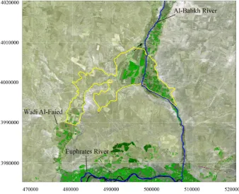
During a short period (13 to 17 January 2007), we conducted a field campaign within Al-Balikh river basin in northern Syria supported by the General Organization for Land Recla-mation, Ar-Raqqa. The campaign covered an area of about 186 km2, between latitude 36◦020to 36◦130N and longitude 38◦460to 39◦030E (Fig. 1).
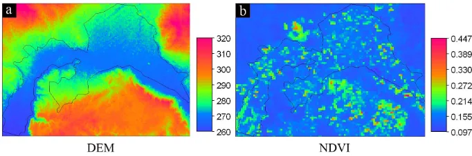
The study area represents a flat region of reclaimed agri-cultural fields. Hence, there is no considerable topographic relief within the area under consideration. The Digital Ele-vation Model retrieved from the ASTER Global Digital El-evation Model (GDEM, 30 m pixel resolution) shows that the level of the flat study area ranges between approximately 260 m and 300 m a.m.s.l. (Fig. 2a).
Fig. 1. Study area location within Al-Balikh river basin in northern of Syria (Google Earth image).
Fig. 2. (a) Digital Elevation Model (30 m pixel resolution), and (b) NDVI map of the study area (250 m pixel resolution).
The area is dominated by steppe climate (K¨oppen climate classification) (Kottek et al., 2006; Peel et al., 2007), which is a semi-dry climate with an average annual rainfall of less than 200 mm. The weather data used in this study was ob-tained from the nearby weather station (Ar-Raqqa, 35◦570N, 39◦000E). The field campaign days were mostly sunny. The prevalent wind was a dry cold northerly wind with an average speed of 2.6 m s−1. In this area, air temperature usually has a high contrast between day and night. During the field cam-paign period, air temperature fell to−5◦C during nighttime and rose to 14◦C during daytime.
Somewhere between mid November and mid February, the main irrigation canal that supplies the whole area is usually blocked for maintenance for about one and half months. A month before our field campaign the irrigation activity had
been stopped. So, we were sure that there were no intense water table fluctuations in the period of our measurements.
[image:3.595.126.467.372.485.2]ranged between 1 and 8 m. Raster maps of soil moisture and water table depth were generated starting from the point data by means of a moving average interpolation.
2.2 Remote sensing data
The MODIS instrument was chosen for our research because it is rich in spectral bands with moderate spatial resolution, and because it provides free-of-charge images at four differ-ent times per day. Currdiffer-ently, there are two operating units of this instrument in space carried by two satellites (Terra and Aqua). Each unit captures images of 36 spectral bands rang-ing in wavelength between 0.4 and 14.4 µm. The numerous bands of MODIS have three spatial resolutions: 250, 500 and 1000 m, and provide data regarding land cover type and dy-namics, vegetation indices, land surface temperature, emis-sivity and albedo.
Two MODIS level 1B images of 17 January 2007 were used in this study as they were the clearest within the field work timeframe. Using the MODIS Reprojection Swath Tool (MRTSwath), each radiances-calibrated level 1B image was transformed from HDF-EOS swath format to a UTM pro-jected GeoTIFF image and resampled into 1 km pixel size. Next, it was imported to the Integrated Land and Water In-formation System (ILWIS) (ITC, 2001) for further process-ing and surface energy balance calculations. This included: raw data to radiance or reflectance transformation; brightness temperature computation and atmospheric correction. Within the framework of SEBS, we calculated the albedo, emissiv-ity and temperature of the land surface, vegetation indices, surface energy fluxes, evaporative fraction and actual daily evaporation.
3 Surface energy balance and related maps calculations
SEBS is an advanced remote sensing algorithm developed by Su (2001) for the estimation of atmospheric turbulent fluxes maps using satellite data. It has been extensively applied and validated with a variety of methods in different regions and climates (Su, 2002; Jia et al., 2003, 2009; Su et al., 2005; McCabe and Wood, 2006; McCabe et al., 2008; Pan et al., 2008; Badola, 2009; van der Kwast et al., 2009; Gibson et al., 2011).
Calculating surface energy fluxes (Eq. 1) by means of SEBS involves using two types of data: spatially distributed variables (maps) and in-situ measured variables. The first type can be derived from remote sensing data and includes land surface albedo, emissivity, temperature, vegetation in-dexes and roughness height. The second type can be obtained from local weather stations and includes air pressure, temper-ature, humidity, wind speed and solar radiation.
Rn =G+H +LE. (1)
The algorithm of SEBS is composed of (1) a set of equa-tions to obtain land surface albedo, emissivity, temperature,
in addition to vegetation indices from satellite data; (2) an extended model for calculating the roughness length for heat transfer; and (3) a formulation for obtaining sensible heat flux by an iterative process.
Net radiation,Rn, is calculated as the outcome of radiation
at land surface:
Rn =(1−α) Kin+ε Lin−ε σ Ts4 (2)
whereKinandLinare the incoming shortwave and longwave
radiations respectively,α,εandTs are land surface albedo,
emissivity and temperature respectively, and σ is Stefan-Boltzmann constant.
Ground heat flux,G, is simply calculated as a ratio of net radiation,Rn, depending on the fractional canopy coverage,
fc, of the studied area:
G=Rn[0.05+0.265(1−fc)]. (3)
Sensible heat flux,H, is calculated using Monin-Obukhov similarity (MOS) theory. The similarity relationships for wind speed and temperature profiles can be expressed as
u= u∗
k
ln
z−d
0
zom
−9m
z−d
0
Ol
+9m
zom
Ol
(4) θs−θa=
H k u∗ρaca
ln
z−d
0
zoh
−9h
z−d
0
Ol
+9h
zoh
Ol
. (5)
uis the average wind speed,θs andθaare the potential
tem-peratures at the land surface and at the reference height,z, respectively,u∗is wind friction velocity,kis von Karman’s
constant,d0is the zero plane displacement height,zomand
zohare the roughness heights for momentum and heat
trans-fer respectively,9mand9hare stability correction functions
for momentum and heat transfer respectively,ρaandca are
air density and specific heat correspondingly and Ol is the Obukhov length.
Sensible heat flux is derived from Eqs. (4) to (5) using an iterative process and latent heat flux is calculated by closing the energy balance (Eq. 1). For further details the reader is referred to Su (2002, 2005).
After estimating all four terms of the surface energy bal-ance (Eq. 1) using SEBS, additional important physical in-formation can be retrieved, such as the daily evaporation, the daily evaporative fraction, and surface soil moisture.
The daily evaporation can be estimated as
Edaily=8.64×107×3×
Rn−G
L ρw
. (6)
In this equation,Lis the latent heat of the vaporization,ρw
is water density. The daily ground heat flux,G, is assumed to be zero, and the daily net radiation,Rn, can be calculated
from
Rn=(1−α) Kin+ε L (7)
whereKinis the daily incoming radiation andLis daily net
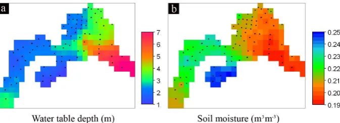
Fig. 3. The interpolated raster maps for (a) water table depth and (b) soil moisture of the upper 5 cm. Locations of the point data collected in the field are also shown.
According to Su (2005), the daily evaporative fraction,3, is conservative and can be approximated by the instantaneous evaporative fraction:
3≈ LE
Rn−G
= LE
LE+H. (8)
The evaporative fraction has proved to be a suitable indicator of soil moisture conditions. Using datasets from the USA and Spain, Bastiaanssen et al. (2000) demonstrated that volumet-ric soil moisture can be estimated using a statistical relation-ship between the evaporative fraction and the soil moisture of the vadose zone. This relationship was later modified by Scott et al. (2003) to involve the degree of saturation (θ/θsat):
θ θsat
=exp
3−1 0.42 (9) whereθandθsatare the actual and the saturated volumetric
soil moisture respectively. By validating the accuracy of this relationship with data from irrigated plains in Pakistan and Mexico, Scott et al. (2003) demonstrated that it is a kind of a standard relationship which can be applied to a wide range of soils. In our calculations, we used a value of 0.49 forθsat
which is the average soil porosity of the predominant top soil in the study area (silty clay).
The spatial relationships between the water table depth and the variant calculated maps were plotted and inspected as de-scribed in the following section.
4 Results and discussion
4.1 Water table depth and soil moisture maps
The two raster maps showing the spatial distributions of the water table depth and the soil moisture were interpolated from the point data collected in the field (Fig. 3). Areas in vicinity to Al-Balikh River (the eastern area) and in Wadi Al-Faied (the south western area) have deeper water table (Fig. 3a) and lower level of soil moisture (Fig. 3b), while the
remaining area has shallower water table and higher level of soil moisture.
The deeper water table conditions in Al-Balikh River and Wadi Al-Faied are most likely attributable to the relatively better drainage conditions. A historical False Color Compos-ite (FCC) image captured by the Multispectral Scanner Sys-tem (MSS) sensor on board of Landsat2 on 8 August 1975 (Fig. 4) demonstrates that the areas with deeper water table correspond to very old cultivated land and that the newly cul-tivated area which has shallower water table suffer poorer drainage conditions.
The cross-relationship between the water table depth and the surface soil moisture is plotted in Fig. 5. It explains that the soil moisture obviously increased starting from a water depth of 4 m upwards. Where the water table was deeper than 4m, the surface soil moisture seems unaffected by water table level.
To insure that the spotted relationship is not indirect and to feature the nature of the water table depth behavior and the spatial distribution of surface soil texture in relation to the land surface elevation, we plotted the water table depth (Fig. 6a), and the texture of the collected soil sam-ples (Fig. 6b) against the land surface elevation. Figure 6a manifests that the shallowest water table (<1.5 m) resides in the areas of highest levels (>285 m a.m.s.l.), and the wa-ter table depth generally tends to increase when the level of land surface decreases. Nevertheless, this increase occurs in two aspects; it can be sharp in some areas (good drainage conditions) and smooth or gradual in others (poor drainage conditions). In addition to these two aspects of the increase, we notice rather a concentrated scattering. The introduction of land reclamation and the accompanying operations such as soil transport and land surface leveling which altered the original hydrological system justifies the two different trends and the scattering in Fig. 6a. The presence of clayey soils detains the lateral water flow and affects the drainage in the newly cultivated areas (Fig. 4).
Fig. 4. Landsat2, False Color Composite (Red = band 5; Green = band 6; Blue = band 4), 8 August 1975, 09:34 LT.
Fig. 5. The cross-relationship between water table depth map and surface soil moisture map.
[image:6.595.49.285.380.537.2]It is noticeable that the sand percentage is low in all samples in comparison to the percentages of silt and clay. However, the silt percentage is to some extent higher than the clay one in the areas of lower surface elevation. Alternatively, the clay percentage is higher that the silt one in the areas of higher surface elevation. Actually, most of the soil samples fall in the silty clay category, and a few fall in the silty clay loam, clay loam, loam and clay categories. Supported by field ob-servations, this limited number of samples provides a rea-sonable prospective about the soil classification in the area.
Figure 6a and b and the relevant discussion infer that soil moisture is potentially affected by the water table depth, and that the influence of topography and soil classification on soil moisture distribution is marginal.
4.2 Soil temperature maps
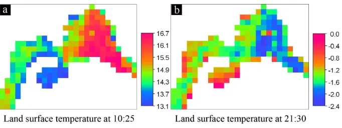
By inspecting both day and night maps of land surface tem-perature extracted from the two MODIS images of 17 Jan-uary 2007, we find that areas of deeper water table depth were warmer during daytime and cooler during nighttime (Fig. 7).
Plotting the cross-relationships (Fig. 8) between the wa-ter table depth and day and night temperatures on 17 Jan-uary 2007 showed that, down to 4 m water depth, the day-time temperature increased (Fig. 8a) while the nightday-time temperature decreased when the water table depth increased (Fig. 8b).
4.3 Surface energy balance maps
Fig. 6. The relationship between land surface elevation and both (a) the water table depth and (b) the soil texture of the collected samples.
Fig. 7. Land surface temperature maps (◦C) of the study area on 17 January 2007. (a) Daytime temperature, and (b) nighttime temperature.
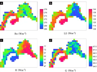
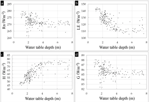
shallow groundwater areas tended to have higher positive net radiation and ground heat flux. The cross-relationships plot-ted in Fig. 10 show that both latent and sensible heat fluxes had a sharper trend to follow the water table depth than net radiation and ground heat flux had. In agreement with the findings and results of the companion paper (Alkhaier et al., 2012), net radiation, latent and ground heat fluxes decreased while sensible heat flux increased when the water table depth increased.
We notice that some pixels within the shallower ground-water areas have lower values than the general trend regard-ing net radiation and ground heat flux (Fig. 10a and d). Inves-tigating the cause of this phenomenon reveals that some spots of these areas suffer soil salinity (Alkhaier, 2003). When ac-cumulating at the land surface, the salt crust increases the albedo (Fujimaki et al., 2003). This in turn magnifies the re-flected shortwave radiation (Eq. 2) and thus diminishes the net radiation.
We notice that ground heat flux is also diminished at these pixels (Fig. 10d). Actually, the behavior of ground heat flux in relation to the water table depth is very similar to that of the net radiation (Fig. 10a and d). This is because SEBS and other surface energy balance algorithms like SEBAL (Basti-aanssen, 1995) simplify the calculation of ground heat flux
by considering it as a ratio of the net radiation, a ratio that depends on the vegetation cover (Eq. 3). In our case, as the vegetation cover was minimal, the spatial variations in both energy components were very similar.
In the companion paper (Alkhaier et al., 2012), we no-tice that the ground heat flux is computed in SHAW (and in many land surface models) by solving for a surface tem-perature that satisfies the complete surface energy balance. The balance equation (Eq. 1) is solved iteratively and simul-taneously with the equations for heat and water fluxes within the soil profile. In SEBS (and other surface energy balance algorithms), we notice that ground heat flux is parameterized and approximated to simplify the calculations. The compar-ison between SHAW and SEBS raises a question regarding the accuracy of the calculated G in SEBS.
Actually the calculation of ground heat flux using Eq. (3), which apparently ignores the soil volumetric heat capacity and thermal conductivity, makes the spatial distribution of
Gand its relationship with water table depth uncertain. The modeling results in the companion paper (Alkhaier et al., 2012: Table 2, and Figs. 3 to 6) reveal that the ratio ofG
toRn not only varies with time but also varies with water
[image:7.595.128.469.262.390.2]Fig. 8. The cross-relationships between the water table depth and both (a) daytime land surface temperatures and (b) nighttime land surface temperatures on 17 January 2007.
Fig. 9. The SEBS calculated maps of the instantaneous components of the surface energy balance, i.e. (a) net radiation; (b) latent heat flux; (c) sensible heat flux; (d) ground heat flux, on 17 January 2007, 10:25 LT.
actual spatial distribution ofG. Further on, since the calcula-tion of the latent heat flux and the derived evaporative terms are dependent on the calculation of the other energy balance terms including ground heat flux, enhancing the calculation of ground heat flux within SEBS will, thereby, enhance the calculation of the evaporative terms.
This discussion point promotes further research to en-hance the calculation ofGin SEBS and other remote sens-ing algorithms. In recent remote senssens-ing studies, there have been some attempts to calculate ground heat flux indepen-dently of net radiation (Murray and Verhoef, 2007). Actually,
integrating such methodologies in SEBS holds a big poten-tial for more accurate mapping of energy fluxes. Neverthe-less, this will require detailed studies, in-situ measurements and calibrations.
4.4 The evaporative fraction and the actual daily evaporation
[image:8.595.128.469.272.525.2]Fig. 10. The cross-relationships between the water table depth and the variant instantaneous components of the surface energy balance, i.e. (a) net radiation; (b) latent heat flux; (c) sensible heat flux; (d) ground heat flux, on 17 January 2007, 10:25 LT.
when the water table depth increased. Comparing the daily evaporation to the measured pan one (Class A) which was recorded by the nearby weather station (2.4 mm) on 17 Jan-uary demonstrates that the SEBS estimates of the energy fluxes are reasonable.
4.5 The soil moisture map estimated from SEBS’ actual daily evaporation
Both soil moisture maps, the one measured in the field and the one estimated from SEBS evaporative fraction, were plot-ted against each other in Fig. 12. This figure manifests a rea-sonable agreement (R2= 0.7506) between soil moisture val-ues from both maps. This agreement demonstrates the rea-sonability of SEBS calculations. However, it is also notice-able that when the values from both maps are low, the esti-mated soil moisture values are slightly lower than the mea-sured ones. But, they are slightly higher when values of both maps are high. We ascribe this to the fact that Eq. (9) was originally developed for soil moisture of the complete vadose zone (Bastiaanssen et al., 2000; Scott et al., 2003), whereas the measured soil moisture values were obtained only for the upper 5 cm of surface soil. In other words, Eq. (9) was
not specifically tailored to the top soil. However, developing this equation to express the top soil moisture is an interest-ing topic to be examined in further studies which inevitably require further measurements and correlation investigations. All in all, this slight difference does not conceal the clear agreement and therefore promotes the effectiveness of re-mote sensing measurements and calculations.
5 Conclusions and recommendations
Fig. 11. The cross-relationships between the water table depth and both (a) the evaporative fraction and (b) the actual daily evaporation.
Fig. 12. The soil moisture of the upper 5 cm measured in field by Stevens’ Hydra probe against the soil moisture estimated from the evaporative fraction using Eq. (9).
Many factors played a substantial role in the good results of our investigation. In view of the conclusions of the com-panion paper (Alkhaier et al., 2012) concerning the favorable conditions for detecting the effect of shallow groundwater via thermal remote sensing, we find that the two major con-ditions were met on this particular day. On the one hand, the effect of latent heat flux was clear at daytime due to the rela-tively high potential evaporation under the prevalent dry and sunny conditions. On the other hand, the effect of volumet-ric heat capacity was clear owing to the high contrast in air temperature between day and night. In this way the circum-stances were most expedient for water table depth detection using thermal remote sensing.
The suspension of irrigation activities together with the scarcity of rainfall for quite some time before the field cam-paign made surface soil moisture and water table depth con-ditions fairly stable. We may add here that the short period
of the campaign facilitated obtaining reliable data of the two state variables (i.e. soil moisture and water table depth).
The limited vegetation cover in the study area was advan-tageous regarding avoiding possible perturbations and com-plexities imposed by plants on surface temperature measuments. Further investigations of such circumstances using re-mote sensing data supported by numerical simulations are recommended.
The limitedness of both topographic relief and vegetation cover in the study area invalidated possible factors of un-certainty in SEBS estimates of energy fluxes (Gibson et al., 2011). Actually, the agreement between the SEBS estimated evaporation and soil moisture values and the field measured values led to the conclusion that the utilization of SEBS in this area under such limitedness was a success.
The exploitation of MODIS in this study proved to be a suitable choice, since it has many convenient characteris-tics. The imaging times were appropriate to detect the ther-mal effect of groundwater at both day and night. Acquir-ing images of an area four times per day secured abundance in imageries, which in turn furnished more options of clear and reliable scenes. Next to the commonly used spectral bands of MODIS for obtaining helpful information about the study area (i.e. vegetation indices, albedo, emissivity, tem-perature, etc.), we found that bands 20 and 22, centered at 3.75 and 3.959 µm respectively, were specifically useful to ascertain that the image was free from perturbation by thin clouds. In terms of its accuracy, precision and resolution, MODIS demonstrated satisfactory efficacy. Even at night-time when land surface temperature ranged within only two degrees Celsius, MODIS could delineate the groundwater ef-fect suitably.
[image:10.595.66.268.271.444.2]sequently all the surface energy balance components. This critical depth may be a peculiarity for this area and may dif-fer from one region to another according to the conditions of the predominant soils.
Some researches suggested developing a procedure for ex-tracting groundwater influence from that of soil moisture (Heilman and Moore, 1982; Huntley, 1978). We believe that this procedure is not necessary if remote sensing investiga-tions are accompanied with appropriate relevant numerical simulations. In fact, the results of this paper together with those of the companion paper (Alkhaier et al., 2012) illus-trate clearly that the two profiles respond differently to rain-falls in a way that they still differ in surface soil moisture. Nevertheless, more attention should be given to the different responses of the two profiles in the periods just after the rain incidents have occurred especially when these incidents are heavy. Right after a heavy rainfall, the effect of groundwater on land surface disappears for some time. Later, the moisture redistributes in the soil profile till the soil moisture profile stabilizes. At this stage, the effect of shallow groundwater on land surface appears again.
The aim of this study is to show the potential of satellites in detecting shallow groundwater. This goal was achieved un-der typical conditions. However, there are some limitations to this method such as intense precipitation, dense vegeta-tion cover and clouds that may make land surface invisible to satellites.
In the companion paper (Alkhaier et al., 2012), we used one-dimensional model simulations to feature the expected behavior of land surface temperature in the presence of a wa-ter table at shallow depths. In this paper, we inspect the re-lationship between the remotely measured land surface tem-perature and the water table depth. The two papers can be considered as one step towards the operational exploitation of satellites in groundwater modeling and studies. However, it is important to point out here that simple correlation anal-ysis will not always be useful to detect the water table depth. There are still many efforts to be exerted to achieve this ob-jective. To put this device (satellites) into operational service for shallow groundwater dynamics, further studies and in-vestigations are required. In our future view of this process, a 3-D transient groundwater model should be involved. This model is recommended to have the capability of simulating the dynamic interaction between water table, surface mois-ture and temperamois-ture. Then, this model can be supported with
US Geological Survey (USGS) Earth Resources Observation and Science (EROS) Center (lpdaac.usgs.gov). The authors highly appreciate the editor Harrie-Jan Hendricks Franssen, and the three anonymous reviewers for their sincere efforts and constructive comments.
Edited by: H.-J. Hendricks Franssen
References
Alkhaier, F.: Soil Salinity Detection Using Satellite Remote Sens-ing, M.Sc. thesis, International Institute for Geo-Information Sci-ence and Earth Observation, The Netherlands, 2003.
Alkhaier, F., Flerchinger, G. N., and Su, Z.: Shallow groundwa-ter effect on land surface temperature and surface energy bal-ance under bare soil conditions: modeling and description, Hy-drol. Earth Syst. Sci., 16, 1817–1831, doi:10.5194/hess-16-1817-2012, 2012.
Badola, A.: Validation of Surface Energy Balance System (SEBS) over Forest Land Cover and Sensitivity Analysis of the Model, M.Sc. thesis, International Institute for Geo-information Science and Earth Observation, The Netherlands, 2009.
Bastiaanssen, W. G. M.: Regionalization of surface flux densities and moisture indicators in composite terrain – A remote sensing approach under clear skies in Mediterranean climates, Ph.D. the-sis, Wageningen Agricultural University, The Netherlands, 1995. Bastiaanssen W. G. M., Molden, D. J., and Makin, I. W.: Remote sensing for irrigated agriculture: examples from research and possible applications, Agr. Water Manage., 46, 137–155, 2000. Becker, M. W.: Potential for satellite remote sensing of ground
wa-ter, Ground Wawa-ter, 44, 306–318, 2006.
Bobba, A. G., Bukata, R. P., and Jerome, J. H.: Digitally processed satellite data as a tool in detecting potential groundwater flow systems, J. Hydrol., 131, 25–62, 1992.
Bosilovich, M., Hook, S., Knuteson, R., Pinheiro, A., Prigent, C., Rossow, W., and Viterbo, P.: International Workshop on the Retrieval and Use of Land Surface Temperature: Bridging the Gaps, Summary Report, NOAA’s National Climatic Data Center (NCDC), Asheville, 7–9 April 2008.
Chase, M. E.: Airborne remote sensing for groundwater studies in prairie environment, Can. J. Earth Sci., 6, 737–741, 1969. Dregne, H. E., Xiong, Z., and Xiong, S.: Soil salinity in China,
De-sertification Control Bull., 28, 28–33, 1996.
Freeze, R. A. and Cherry, J. A.: Groundwater, Prentice-Hall, Inc. Englewood Cliffs, NJ, 1979.
Fujimaki, H., Shiozawa, S., and Inoue, M.: Effect of salty crust on soil albedo, Agr. Forest. Meteorol., 118, 125–135, doi:10.1016/S0168-1923(03)00110-2, 2003.
Gibson, L. A., M¨unch, Z., and Engelbrecht, J.: Particular uncertain-ties encountered in using a pre-packaged SEBS model to derive evapotranspiration in a heterogeneous study area in South Africa, Hydrol. Earth Syst. Sci., 15, 295–310, doi:10.5194/hess-15-295-2011, 2011.
Heilman, J. L. and Moore, D. G.: Evaluating depth to shallow groundwater using heat capacity mapping mission (HCMM) data, Photogramm. Eng. Rem. S., 48, 1903–1906, 1982. Huntley, D.: On the detection of shallow aquifers using thermal
in-frared imagery, Water Resour. Res., 14, 1075– 1083, 1978. ITC: ILWIS 3.0 Academic user’s guide, International institute for
aerospace survey and earth sciences, Enschede, The Netherlands, 2001.
Jia, L., Su, Z., van den Hurk, B., Menenti, M., Moene, A., de Bruin, H. A. R., Yrisarry, J. J. B., Ibanez, M., and Cuesta, A.: Estimation of sensible heat flux using the Surface Energy Balance System (SEBS) and ATSR measurements, Phys. Chem. Earth, 28, 75– 88, 2003.
Jia, L., Xi, G., Liu, S., Huang, C., Yan, Y., and Liu, G.: Re-gional estimation of daily to annual reRe-gional evapotranspira-tion with MODIS data in the Yellow River Delta wetland, Hy-drol. Earth Syst. Sci., 13, 1775–1787, doi:10.5194/hess-13-1775-2009, 2009.
Kottek, M., Grieser, J., Beck, C., Rudolf, B., and Rubel, F.: World Map of the K¨oppen-Geiger climate classification updated, Mete-orol. Z., 15, 259–263, doi:10.1127/0941-2948/2006/0130, 2006. McCabe, M. F. and Wood, E. F.: Scale influences on the remote estimation of evapotranspiration using multiple satellite sensors, Remote Sens. Environ., 105, 271–285, 2006.
McCabe, M. F., Wood, E. F., Wojcik, R., Pan, M., Sheffield, J., Gao, H., and Su, H.: Hydrological consistency using multi-sensors re-mote sensing data for water and energy cycle studies, Rere-mote Sens. Environ., 112, 430–444, 2008.
Meijerink, A. M. J., Bannert, D., Batelaan, O., Lubczynski, M. W., and Pointet, T.: Remote Sensing Applications to Groundwater, Paris, United Nations Educational Scientific and Cultural Orga-nization (UNESCO), 2007.
Middleton, N. and Thomas, D.: World Atlas of Desertification, 2, Wiley, publisher Arnold United Nations Environment Pro-gramme (UNEP), New York, 1997.
Murray, T. and Verhoef, A.: Moving towards a more mechanistic approach in the determination of soil heat flux from remote mea-surements, II: Diurnal shape of soil heat flux, Agr. Forest. Mete-orol., 147, 88–97, 2007.
Myers, V. I. and Moore, D. G.: Remote sensing for defining aquifers in glacial drift, Eighth International Symposium on Remote Sensing of Environment, 1, University of Michigan, 715–728, 1972.
Northey, J. E., Christen, E. W., Ayars, J. E., and Jankowski, J.: Oc-currence and measurement of salinity stratification in shallow groundwater in the Murrumbidgee Irrigation Area, south-eastern Australia, Agr. Water Manage., 81, 23–40, 2006.
Pan, M., Wood, E. F., Wojcik, R., and McCabe, M. F.: Estimation of regional terrestrial water cycle using multi-sensor remote sensing observations and data assimilation, Remote Sens. Environ., 112, 1282–1294, 2008.
Peel, M. C., Finlayson, B. L., and McMahon, T. A.: Updated world map of the K¨oppen-Geiger climate classification, Hy-drol. Earth Syst. Sci., 11, 1633–1644, doi:10.5194/hess-11-1633-2007, 2007.
Rahman, A.: A GIS based DRASTIC model for assessing ground-water vulnerability in shallow aquifer in Aligarh, India, Appl. Geogr., 28, 32–53, 2008.
Scott, C. A., Bastiaanssen, W. G. M., and Ahmad, M. D.: Map-ping spatio-temporal distributions of soil moisture throughout ir-rigated watersheds using optical and high resolution imagery, J. Irrig. Drain. Eng.-ASCE, 129, 326–335, 2003.
Su, H., McCabe, M. F., and Wood, E. F.: Modeling evapotranspira-tion during SMACEX: Comparing two approaches for local and regional-scale prediction, J. Hydrometeorol. – Special Section, 6, 910–922, 2005.
Su, Z.: A Surface Energy Balance System (SEBS) for estimation of turbulent heat fluxes from point to continental scale, Publi-cations of the National Remote Sensing Board (BCRS), USP-2, The Netherlands, 2001.
Su, Z.: The Surface Energy Balance System (SEBS) for estima-tion of turbulent heat fluxes, Hydrol. Earth Syst. Sci., 6, 85–100, doi:10.5194/hess-6-85-2002, 2002.
Su, Z.: Estimation of the surface energy balance, in: Encyclopedia of Hydrological Sciences, edited by: Anderson, M. G. and Mc-Donnell, J. J., 2, Wiley and Sons, 731–752, 2005.
Umali, D. L.: Irrigation-Induced Salinity: A Growing Problem for Development and the Environment, Technical Paper 215, World Bank, Washington, D.C., 1993.
van der Kwast, J., Timmermans, W., Gieske, A., Su, Z., Olioso, A., Jia, L., Elbers, J., Karssenberg, D., and de Jong, S.: Eval-uation of the Surface Energy Balance System (SEBS) applied to ASTER imagery with flux-measurements at the SPARC 2004 site (Barrax, Spain), Hydrol. Earth Syst. Sci., 13, 1337–1347, doi:10.5194/hess-13-1337-2009, 2009.
Wichelns, D.: An economic model of waterlogging and salinization in arid regions, Ecol. Econ., 30, 475–491, 1999.
World Bank: Development and the Environment, World Develop-ment Report, World Bank, Washington, D.C., 1992.