On the \(O(1/t)\) convergence rate of the alternating direction method with LQP regularization for solving structured variational inequality problems

R E S E A R C H

Open Access

On the

O

(/

t

)

convergence rate of the

alternating direction method with LQP

regularization for solving structured

variational inequality problems

Abdellah Bnouhachem

_{, Abdul Latif}

_{and Qamrul Hasan Ansari}

*_{Correspondence:}

[email protected]

1_{School of Management Science}

and Engineering, Nanjing University, Nanjing, 210093, P.R. China

2_{Laboratoire d’Ingénierie des}

Systémes et Technologies de l’Information, ENSA, Ibn Zohr University, Agadir, BP 1136, Morocco Full list of author information is available at the end of the article

†_{Equal contributors}

Abstract

In this paper, we propose a parallel descent LQP alternating direction method for solving structured variational inequality with three separable operators. TheO(1/t) convergence rate for this method is studied. We also present some numerical examples to illustrate the efficiency of the proposed method. The results presented in this paper extend and improve some well-known results in the literature.

MSC: Primary 90C33; 49J40; secondary 65N30

Keywords: structured variational inequalities; logarithmic-quadratic proximal method; convergence rate; projection method; alternating direction method

1 Introduction

LetRn

+={x= (x,x, . . . ,xn)∈Rn:xi≥∀i= , , . . . ,n} andRn++={x= (x,x, . . . ,xn)∈

Rn_:x

i> ∀i= , , . . . ,n}. The variational inequality problem is to find

x∈:=(u,v) :u∈Rn₊,v∈Rm₊,Au+Av=b

such that

x–xTF(x)≥, ∀x∈, (.)

with

x=

u v

and F(x) =

f(u)

f(v)

, (.)

whereA∈Rl×n,A∈Rl×mare given matrices,b∈Rlis a given vector, andf:Rn+→Rn,

f:Rm+ →Rm are given monotone operators. For further study and applications of such problems, we refer to [–] and the references therein. By attaching a Lagrange multi-plier vectorλ∈Rl_{to the linear constraintsA}

u+Av=b, the problem (.)-(.) can be

explained in terms of findingz∈Z:=Rn

+×Rm+ ×Rlsuch that

z–zQ(z)≥, ∀z∈Z, (.)

where

z=

⎛ ⎜ ⎝

u v

λ

⎞ ⎟

⎠, Q(z) =

⎛ ⎜ ⎝

f(u) –Aλ

f(v) –Aλ

Au+Av–b

⎞ ⎟

⎠, (.)

andA_ denotes the transpose of the matrixA. The problem (.)-(.) is referred as a

structured variational inequality problem(in short, SVI).

Yuan and Li [] developed the following logarithmic-quadratic proximal (LQP)-based decomposition method by applying the LQP terms to regularize the ADM subprob-lems: For a given zk _{= (u}k_,vk_,λk_)∈Rn

++×Rm++×Rl, and μ∈(, ), the new iterative (uk+_,vk+_,λk+_{) is obtained via solving the following system:}

f(u) –A

λk–HAu+Avk–b

+Ru–uk+μuk–U_ku–= , (.)

f(v) –A

λk–H(Au+Av–b)

+Sv–vk+μvk–V_kv–= , (.)

λk+=λk–HAuk+Avk–b

, (.)

whereH∈Rl×l,R∈Rn×n, andS∈Rm×mare symmetric positive definite.

Later, some LQP alternating direction methods have been proposed to make the LQP alternating direction method more practical, see, for example, [–] and the references therein. Each iteration of these methods contains a prediction and a correction, the pre-dictor is obtained via solving (.)-(.) and the new iterate is obtained by a convex com-bination of the previous point and the one generated by a projection-type method along a descent direction. The main disadvantage of the methods proposed in [–] is that solving equation (.) requires the solution of equation (.). To overcome with this diffi-culty, Bnouhachem and Hamdi [] proposed a parallel descent LQP alternating direction method for solving SVI.

In this paper, we propose a parallel descent LQP alternating direction method for solving the following structured variational inequality with three separable operators: Findy∈

:={(u,v,w) :u∈Rn

+,v∈Rn+,w∈Rn+,Au+Av+Aw=b}such that

y–yF(y)≥, ∀y∈, (.)

with

y=

⎛ ⎜ ⎝

u v w

⎞ ⎟

⎠, F(y) =

⎛ ⎜ ⎝

f(u)

f(v)

f(w)

⎞ ⎟

⎠, (.)

whereA∈Rm×n,A∈Rm×n,A∈Rm×n are given matrices,b∈Rmis a given vector, andf:Rn+→Rn,f:R+n →Rn,f:Rn+ →Rn are given monotone operators. By at-taching a Lagrange multiplier vectorλ∈Rm_{to the linear constraintsA}

the problem (.)-(.) can be explained in terms of findingz∈Z:=Rn

+ ×Rn+×Rn+×Rm such that

z–zQ(z)≥, ∀z∈Z, (.)

where

z=

⎛ ⎜ ⎜ ⎜ ⎝

u v w

λ

⎞ ⎟ ⎟ ⎟

⎠ and Q(z) =

⎛ ⎜ ⎜ ⎜ ⎝

f(u) –Aλ

f(v) –Aλ

f(w) –Aλ

Au+Av+Aw–b

⎞ ⎟ ⎟ ⎟

⎠. (.)

The problem (.)-(.) is referred as SVI.

The main aim of this paper is to present the parallel descent LQP alternating direction method for solving SVIand to investigate the convergence rate of this method. We show that the proposed method has theO(/t) convergence rate. The iterative algorithm and results presented in this paper generalize, unify, and improve the previously known results in this area.

2 The proposed method

For any vectoru∈Rn_,u∞=max{|u

|, . . . ,|un|}. LetD∈Rn×nbe a symmetry positive definite matrix, we denote theD-norm ofubyu_D=uTDu.

The following lemma provides a basic property of projection operator onto a closed convex subsetofRl_{. We denote byP}

,D(·) the projection operator under theD-norm, that is,

P,D(v) =argmin

v–uD:u∈

.

Lemma . Let D be a symmetry positive definite matrix and be a nonempty closed convex subset ofRl_.Then

z–P,D[z]

DP,D[z] –v

≥, ∀z∈Rl,v∈. (.)

We make the following standard assumptions.

Assumption . f is monotone with respect toRn+, that is, (f(x) –f(y))T(x–y)≥,

∀x,y∈Rn

+,fis monotone with respect toRn+, andfis monotone with respect toRn+.

Assumption . The solution set of SVI, denoted byZ∗, is nonempty.

We propose the following parallel LQP alternating direction method for solving SVI:

Algorithm .

Step . Givenε> ,μ∈(, ),β∈( √



 , ),γ ∈(, )and

z_{= (u}_,v_,w_,λ_)∈Rn

Step . Computez˜k_{= (u˜}k_,v˜k_,w˜k_,λ˜k_)∈Rn

++×Rn++ ×Rn++ ×Rmby solving the following

system:

f(u) –A

λk–HAu+Avk+Awk–b

+R

u–uk+μuk–U_ku–= , (.)

f(v) –A

λk–HAuk+Av+Awk–b

+R

v–vk+μvk–V_kv–= , (.)

f(w) –A

λk–HAuk+Avk+Aw–b

+R

w–wk+μwk–W_kw–= , (.)

˜

λk=λk–βHAu˜k+Av˜k+Aw˜k–b

, (.)

whereH∈Rm×m,R∈Rn×n,R∈Rn×n andR∈Rn×nare symmetric

positive definite matrices.Uk,Vk, andWkare positive definite diagonal matrices defined byUk=diag(uk, . . . ,ukn),Vk=diag(vk, . . . ,vkn),Wk=diag(wk, . . . ,wkn). Step . Ifmax{uk–u˜k∞,vk–v˜k∞,wk–w˜k∞,λk–λ˜k∞}<, then stop. Step . The new iteratezk+(τk) = (uk+,vk+,wk+,λk+)is given by

zk+(τk) = ( –σ)zk+σPZ,G

zk–γ τkG–g

zk,z˜k, σ∈(, ), (.)

where

τk=

ϕ(zk_,z˜k₎ zk_–z˜k

G

, (.)

ϕzk,z˜k=zk–˜zk_M

+ β

λk–λ˜kTA

uk–u˜k+A

vk–˜vk+A

wk–w˜k, (.)

g(zk_,z˜k₎

= ⎛ ⎜ ⎜ ⎜ ⎝

f(u˜k) –Aλ˜k+AH[A(uk–u˜k) +A(vk–v˜k) +A(wk–w˜k) +–ββH

–_(λk_–λ˜k_)] f(v˜k) –Aλ˜k+AH[A(uk–u˜k) +A(vk–v˜k) +A(wk–w˜k) +–ββH

–_(λk_–λ˜k_)] f(w˜k) –Aλ˜k+AH[A(uk–u˜k) +A(vk–v˜k) +A(wk–w˜k) +–ββH

–_(λk_–λ˜k_)] Au˜k+Av˜k+Aw˜k–b

⎞ ⎟ ⎟ ⎟ ⎠,

(.)

G= ⎛ ⎜ ⎜ ⎝

( +μ)R+A_HA   

 ( +μ)R+AHA  

  ( +μ)R+AHA 

   

βH

–

⎞ ⎟ ⎟ ⎠,

and

M=

⎛ ⎜ ⎜ ⎜ ⎝

R+AHA   

 R+AHA  

  R+AHA 

   _βH–

⎞ ⎟ ⎟ ⎟ ⎠.

Remark . As special cases, we can obtain some new LQP alternating methods as fol-lows:

(a) Ifuk+=u˜k,vk+=v˜k,wk+=w˜kandλk+=λ˜kin (.), (.), (.) and (.), respectively, we obtain a new method which can be viewed as an extension of that proposed in [] for solving structured variational inequality with three separable operators in a parallel way.

(b) Ifuk+_=u˜k_,vk+_=v˜k_,wk+_=w˜k_,λk+_=λ˜k_{, andβ= in (.), (.), (.) and (.),} respectively, we obtain a new method which can be viewed as an extension of that proposed in [] for solving structured variational inequality with three separable operators in a parallel wise.

(c) Ifβ= , the proposed method can be viewed as an extension of that proposed in [] for solving structured variational inequality with three separable operators.

We need the following result in the convergence analysis of the proposed method.

Lemma .([]) Let q(u)∈Rn_{be a monotone mapping of u with respect toR}n

+and R∈

Rn×n_{be a positive definite diagonal matrix.For a given u}k_{> ,if U}

k:=diag(uk,uk, . . . ,ukn) (the diagonal matrix with elements uk_,uk_, . . . ,uk

n)and u–be an n-vector whose jth element

is/uj,then the equation

q(u) +Ru–uk+μuk–U_ku–=  (.)

has a unique positive solution u.Moreover,for any v≥,we have

(v–u)q(u)≥ +μ 

u–v_R–uk–v_R+ –μ  u

k_–u

R. (.)

The next theorem is useful for the convergence analysis.

Theorem . For given zk_∈Rn

++×Rn++×Rn++×Rm,letz˜kbe generated by(.)-(.).Then

ϕzk,z˜k≥β– √

 β z

k_–z˜k

G (.)

and

τk≥

β–√

β . (.)

Proof It follows from (.) that

ϕzk,z˜k=zk–˜zk_M+  β

λk–λ˜kA

uk–u˜k+A

vk–˜vk+A

wk–w˜k

=uk–u˜k_R

+Au k_–A

u˜k  H+v

k_–v˜k

R+Av k_–A

v˜k  H

+wk–w˜k_R

+Aw k_–A

w˜k  H+

 βλ

k_–λ˜k H–

+  β

λk–λ˜kA

uk–u˜k+A

vk–v˜k+A

By using the Cauchy-Schwarz inequality, we have

λk–λ˜kA

uk–u˜k≥– 

_√

A

uk–u˜k_H+√ λ

k_–λ˜k H–

, (.)

λk–λ˜kA

vk–v˜k≥– 

_√

A

vk–v˜k_H+√ λ

k_–λ˜k H–

, (.)

and

λk–λ˜kA

wk–w˜k≥– 

_√

A

wk–w˜k_H+√ λ

k_–λ˜k H–

. (.)

Substituting (.), (.), and (.) into (.), we get

ϕzk,z˜k≥β– √

 β Au

k_–A u˜k

 H+Av

k_–A v˜k



H+Aw k_–A

w˜k  H + – √  β λ

k_–λ˜k

H–+uk–u˜k  R+v

k_–v˜k R+w

k_–w˜k R

≥β– √

 β

Auk–Au˜k  H+Av

k_–A v˜k

 H

+Awk–Aw˜k_H+  βλ

k_–λ˜k H–

+β– √

 β u

k_–u˜k R+v

k_–˜vk R+w

k_–w˜k R

= β– √

 β z

k_–z˜k

G+ ( –μ)u k_–u˜k

R

+ ( –μ)vk_–v˜k

R+ ( –μ)w k_–w˜k

R

≥β– √

 β z

k_–z˜k G.

Therefore, it follows from (.) and (.) that

τk≥

β–√

β , (.)

and this completes the proof.

3 Convergence rate

Recall thatZ∗can be characterized as (see (..) in p. of [])

Z∗₌ z∈Z

ˆ

z∈Z: (z–zˆ)Q(z)≥.

This implies thatˆzis an approximate solution of SVIwith the accuracy>  if it satisfies

ˆ

z∈Z and sup

z∈Z

Now we show that aftertiterations of the proposed method, we can find aˆz∈Zsuch that (.) is satisfied with=O(/t).

We introduce the following matrices,

N=

⎛ ⎜ ⎜ ⎜ ⎝

I   

 I  

  I 

–βHA –βHA –βHA βI

⎞ ⎟ ⎟ ⎟

⎠ (.)

and

J=

⎛ ⎜ ⎜ ⎜ ⎝

( +μ)R+AHA   

 ( +μ)R+AHA  

  ( +μ)R+AHA 

–A –A –A H–

⎞ ⎟ ⎟ ⎟

⎠. (.)

By simple manipulations, we can find thatJ=GN. Our analysis needs a new sequence defined by

ˆ zk=

⎛ ⎜ ⎜ ⎜ ⎝

ˆ uk ˆ vk ˆ wk

ˆ λk

⎞ ⎟ ⎟ ⎟

⎠=

⎛ ⎜ ⎜ ⎜ ⎝

˜ uk ˜ vk ˜ wk

λk–H(Auk+Avk+Awk–b)

⎞ ⎟ ⎟ ⎟

⎠. (.)

Based on (.) and (.), we can easily have

zk–z˜k=Nzk–zˆk. (.)

Using (.), (.), and (.), we obtain

gzk,z˜k=Qˆzk. (.)

Lemma . Letˆzkbe defined by(.),z∈Z,and the matrix J be given by(.).Then

z–zˆkQˆzk–Jzk–zˆk≥–μuk–uˆk_R

–μv k_–vˆk

R–μw k_–wˆk

R. (.)

Proof Applying Lemma . to (.), we get

u–u˜kf

˜

uk–A_λk–HAu˜k+Avk+Awk–b

≥ +μ  u˜

k_–u R–u

k_–u R

+ –μ  u

k_–u˜k

R. (.)

Since

uk–u_R

=u k_–u˜k

R+u˜ k_–u

R+ 

˜

uk–uTR

uk–u˜k,

we have

u–u˜kR

uk–u˜k= u˜

k_–u R–u

k_–u R

+ u

k_–u˜k

Adding (.) and (.), we obtain

u–u˜k( +μ)R

uk–u˜k–f

˜

uk+A_λk–HAuk+Avk+Awk–b

+A_HA

uk–u˜k≤μuk–u˜k_R

. (.)

Similarly, applying Lemma . to (.), we get

v–v˜kf

˜

vk–A_λk–HAuk+A˜vk+Awk–b

≥ +μ  v˜

k_–v R–v

k_–v R

+ –μ  v

k_–v˜k

R. (.)

Similar to (.), we have

v–v˜kR

vk–v˜k= v˜

k_–v R–v

k_–v R

+ v

k_–v˜k

R. (.)

Adding (.) and (.), we have

v–v˜k( +μ)R

vk–v˜k–f

˜

vk+A_λk–HAuk+Avk+Awk–b

+A_HA

vk–v˜k≤μvk–v˜k_R

. (.)

Similarly, we have

w–w˜k( +μ)R

wk–w˜k–f

˜

wk+A_λk–HAuk+Avk+Awk–b

+A_HA

wk–w˜k≤μwk–w˜k_R

. (.)

Then, by using the notation ofˆzk_{in (.), (.), (.), and (.) can be written as}

u–uˆk( +μ)R

uk–uˆk–f(uˆk) +Aλˆk+AHA

uk–uˆk

≤μuk–uˆk_R

, (.)

v–vˆk( +μ)R

vk–vˆk–f

ˆ

vk+A_λˆk+A_HA

vk–vˆk

≤μvk–vˆk_R

, (.)

and

w–wˆk( +μ)R

wk–wˆk–f

ˆ

wk+A_λˆk+A_HA

wk–wˆk

≤μwk–wˆk_R

. (.)

In addition, it follows from (.) that

Auˆk+Avˆk+Awˆk–b+H–

_ˆ

λk–λk

–A

ˆ

uk–uk–A

ˆ

vk–vk–A

ˆ

Combining (.)-(.), we get

⎛ ⎜ ⎜ ⎝

u–uˆk v–vˆk w–wˆk

λ–λˆk ⎞ ⎟ ⎟ ⎠ ⎛ ⎜ ⎜ ⎝

f(uˆk) –Aλˆk– (( +μ)R+ATHA)(uk–uˆk)

f(vˆk) –Aλˆk– (( +μ)R+AHA)(vk–vˆk)

f(wˆk) –Aλˆk– (( +μ)R+AHA)(wk–wˆk)

Auˆk+Aˆvk+Awˆk–b+A(uk–uˆk) +A(vk–vˆk) +A(wk–wˆk) –H–(λk–λˆk)

⎞ ⎟ ⎟ ⎠

≥–μuk_–uˆk

R–μv

k_–vˆk

R–μw

k_–wˆk

R. (.)

Recall the definition ofJin (.), we obtain the assertion (.). The proof is completed.

Lemma . For given zk_∈Rn

++×Rn++ ×R++n ×Rmand zk∗:=PZ,G[zk–τkG–g(zk,˜zk)],we

have

γ τk

z–zˆkQ(z) +  z–z

k

G–z–z k ∗G

≥ 

γ( –γ)τ 

kzk–z˜k 

G. (.)

Proof Sincezk

∗∈Z, substitutingz=z∗kin (.), we get

γ τk

z_∗k–zˆkQzˆk (.)

≥γ τk

z_∗k–zˆkJzk–zˆk–μγ τkuk–uˆk 

R–μγ τkv k_–vˆk

R

–μγ τkwk–wˆk  R

=γ τkzk–zˆkJzk–zˆk+γ τkzk_∗–zkJzk–zˆk

–μγ τkuk–uˆk_R

–μγ τkv k_–vˆk

R–μγ τkw k_–wˆk

R

=γ τk

zk–z˜kN–JN–zk–z˜k+γ τk

zk_∗–zkJN–zk–z˜k

–γ τkμuk–uˆk 

R–γ τkμv k_–vˆk

R–μγ τkw k_–wˆk

R

=γ τk

zk–z˜kN–Gzk–z˜k–γ τkμuk–uˆk 

R–γ τkμv k_–vˆk

R

–μγ τkwk–wˆk_R +γ τk

zk_∗–zkGzk–z˜k

=γ τk

zk–z˜kN–Mzk–z˜k+γ τk

zk_∗–zkGzk–z˜k

≥γ τkϕ

zk,˜zk+γ τk

z_∗k–zkGzk–˜zk

≥γ τkϕ

zk,˜zk– z

k_–zk ∗G–

 γ

_τ

kzk–z˜k  G

=

γ( –γ)τ 

kzk–z˜k  G–

 z

k_–zk

∗G. (.)

Using (.),zk_∗is the projection ofzk–γ τkG–Q(zˆk) onZ, it follows from (.) that

zk–γ τkG–Q

ˆ

zk–zk_∗Gz–zk_∗≤, ∀z∈Z,

and consequently, we have

γ τk

Using the identityxGy= _(x

G–x–yG+yG) to the right hand side of the last inequality, we obtain

γ τk

z–zk ∗

Qzˆk_≥  z–z

k

∗G–z–z k

G

+ z

k_–zk

∗G. (.)

Adding (.) and (.), we get

γ τkz–zˆkQzˆk+ z–z

k

G–z–z k ∗G

≥ 

γ( –γ)τ 

kzk–z˜k  G,

and by using the monotonicity ofQ, we obtain (.) and the proof is completed.

Lemma . Let zk_∈Rn

++×Rn++ ×Rn++ ×Rmand zk+(τk)be generated by(.).Then

γ σ τk

z–ˆzkQ(z) + z–z

k

G–z–z k+_(τ

k)  G

≥ 

σ γ( –γ)τ  kz–z˜k

 G. (.)

Proof We have

z–zk_G–z–zk+(τk) 

G (.)

=zk–z_G–zk–σzk–zk_∗–z_G

= σzk–zGzk–zk_∗–σzk–zk_∗_G

= σzk–zk_∗G –z–zk_∗Gzk–zk_∗–σzk–zk_∗_G. (.)

Using the identity

z–zk_∗Gzk–zk_∗= z

k

∗–zG–z k_–z

G

+ z

k_–zk ∗G,

we get

zk–zk_∗_G– z–zk_∗Gzk–zk_∗=zk–z_G–zk_∗–z_G. (.)

Substituting (.) into (.), we obtain

z–zk_G–z–zk+(τk) 

G =σz–z k

G–z–z k ∗G

+σ( –σ)zk–zk_∗_G

≥σz–zk_G–z–zk_∗_G. (.)

Substituting (.) into (.), we obtain (.), the required result.

Theorem . Let z∗be a solution ofSVIand zk+(τk)be generated by(.).Then zkand ˜

zk_{are bounded,and}

zk+(τk) –z∗_G≤zk–z∗_G–czk–˜zk_G, (.)

where

c:=σ γ( –γ)(β– √

Proof Settingz=z∗in (.), we obtain

zk+(τk) –z∗  G≤z

k_–z∗

G–σ γ( –γ)τ 

kzk–z˜k 

G+ γ σ τk

z∗–zˆkQz∗

≤zk–z∗_G–σ γ( –γ)τ_kzk–z˜k_G

≤zk–z∗_G–σ γ( –γ)(β– √

)

β z

k_–˜zk G.

Then we have

zk+(τk) –z∗_G≤zk–z∗_G≤ · · · ≤z–z∗_G,

and thus,{zk}is a bounded sequence. It follows from (.) that

∞

k=

czk–˜zk_G< +∞,

which means that

lim k→∞z

k_–z˜k

G= . (.)

Since{zk_{}is a bounded sequence, we conclude that{˜z}k_{}is also bounded.} The global convergence of the proposed method can be proved by similar arguments as in []. Hence the proof is omitted.

Theorem . The sequence{zk_{}generated by the proposed method converges to some z}∞

which is a solution ofSVI.

Now, we are ready to present theO(/t) convergence rate of the proposed method.

Theorem . For any integer t> ,we have azˆt∈Zwhich satisfies

(zˆt–z)Q(z)≤  γ σ ϒt

z–z_G, ∀z∈Z,

where

ˆ zt=

 ϒt

t

k=

τkˆzk and ϒt= t

k= τk.

Proof Summing the inequality (.) overk= , . . . ,t, we obtain

_t

k= γ σ τk

z– t

k= γ σ τkˆzk

Q(z) + z–z

Using the notations ofϒtandzˆtin the above inequality, we derive

(zˆt–z)Q(z)≤ 

γ σ ϒtz–z 

G, ∀z∈Z.

Indeed, ˆzt∈Z because it is a convex combination of zˆ,zˆ, . . . ,zˆt. The proof is

com-pleted.

Remark . It follows from (.) that

ϒt≥

β–√ β (t+ ).

Suppose that, for any compact setD⊂Z, letd=sup{z–z

G|z∈D}. For any given> , after at most

t=

βd

(β–√)γ σ

iterations, we have

(zˆt–z)TQ(z)≤, ∀z∈D.

That is, theO(/t) convergence rate is established in an ergodic sense.

4 Preliminary computational results

In this section, we present some numerical examples to illustrate the proposed method. We consider the following optimization problem with matrix variables, which is studied in []:

min



U–C  FU∈Sn+

, (.)

where · Fis the matrix Fröbenius norm,i.e.,CF= (ni=

n

j=|Cij|)/and

Sn₊=M∈Rn×n:M=M,M.

It has been shown in [] that solving problem (.) is equivalent to the following varia-tional inequality problem: FindX∗= (U∗,V∗,Z∗)∈=Sn

+×Sn+×Rn×nsuch that

⎧ ⎪ ⎪ ⎨ ⎪ ⎪ ⎩

U–U∗, (U∗–C) –Z∗ ≥,

V–V∗, (V∗–C) +Z∗ ≥, ∀X= (U,V,Z)∈, U∗–V∗= .

(.)

The problem (.) is a special case of (.)-(.) with matrix variables whereA=In×n,

Table 1 Numerical results for problem (4.1) withr1= 0.5,r2= 5

Dimension of the problem

The proposed method The method in [18] The method in [17]

k CPU (Sec.) k CPU (Sec.) k CPU (Sec.)

100 43 0.83 49 0.96 71 2.47

300 48 3.98 53 4.85 79 6.33

500 50 11.54 56 13.27 82 20.2

700 52 29.91 57 34.33 85 44.06

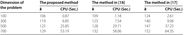
Table 2 Numerical results for problem (4.1) withr₁= 1,r₂= 10

Dimension of the problem

The proposed method The method in [18] The method in [17]

k CPU (Sec.) k CPU (Sec.) k CPU (Sec.)

100 106 0.87 109 1.18 124 2.61

300 119 6.85 123 7.54 140 9.06

500 125 25.85 128 29.71 147 37.25

700 129 53.19 132 58.06 152 64.35

we takeμ= .,β = .,C=rand(n), and (U,V,Z) = (In×n,In×n, n×n) as the initial point in the test. The iteration is stopped as soon as

maxUk–U˜k,Vk–V˜k,Zk–Z˜k≤–.

All codes were written in Matlab, we compare the proposed method with those in [] and []. The iteration numbers, denoted byk, and the computational time for the problem (.) with different dimensions are given in Tables -.

Tables - show that the proposed method is more flexible and efficient for the problem tested.

5 Conclusions

In this paper, we proposed a new modified logarithmic-quadratic proximal alternating direction method for solving structured variational inequalities with three separable op-erators. The prediction point is obtained by solving series of related systems of nonlinear equations in a parallel way. Global convergence of the proposed method is proved under mild assumptions. We have proved theO(/t) convergence rate of the parallel LQP alter-nating direction method. Some preliminary numerical examples are reported to verify the effectiveness of the proposed method in practice.

Competing interests

The authors declare that they have no competing interests.

Authors’ contributions

All authors contributed equally and significantly in writing this article. All authors read and approved the final manuscript.

Author details

1_{School of Management Science and Engineering, Nanjing University, Nanjing, 210093, P.R. China.}2_Laboratoire

d’Ingénierie des Systémes et Technologies de l’Information, ENSA, Ibn Zohr University, Agadir, BP 1136, Morocco.

3_{Department of Mathematics, King Abdulaziz University, P.O. Box 80203, Jeddah 21589, Saudi Arabia.}4_{Department of}

Mathematics, Aligarh Muslim University, Aligarh 202002, India.5_{Department of Mathematics & Statistics, King Fahd}

University of Petroleum & Minerals, Dhahran, Saudi Arabia.

Acknowledgements

third author was done during his visit to King Fahd University of Petroleum & Minerals (KFUPM), Dhahran, Saudi Arabia. He is grateful to KFUPM for providing excellent research facilities to carry out his part of this research.

Received: 3 October 2016 Accepted: 8 November 2016 References

1. Fortin, M, Glowinski, R: Augmented Lagrangian Methods: Applications to the Solution of Boundary-Valued Problems. North-Holland, Amsterdam (1983)

2. Gabay, D: Applications of the method of multipliers to variational inequalities. In: Fortin, M, Glowinski, R (eds.) Augmented Lagrangian Methods: Applications to the Solution of Boundary-Valued Problems. Studies in Mathematics and Its Applications, vol. 15, pp. 299-331. North-Holland, Amsterdam, The Netherlands (1983) 3. Gabay, D, Mercier, B: A dual algorithm for the solution of nonlinear variational problems via finite-element

approximations. Comput. Math. Appl.2, 17-40 (1976)

4. Glowinski, R: Numerical Methods for Nonlinear Variational Problems. Springer, New York (1984)

5. Glowinski, R, Le Tallec, P: Augmented Lagrangian and Operator-Splitting Methods in Nonlinear Mechanics. SIAM Studies in Applied Mathematics. SIAM, Philadelphia, PA (1989)

6. He, BS, Yang, H: Some convergence properties of a method of multipliers for linearly constrained monotone variational inequalities. Oper. Res. Lett.23, 151-161 (1998)

7. Hou, LS: On theO(1/t) convergence rate of the parallel descent-like method and parallel splitting augmented Lagrangian method for solving a class of variational inequalities. Appl. Math. Comput.219, 5862-5869 (2013) 8. Jiang, ZK, Bnouhachem, A: A projection-based prediction-correction method for structured monotone variational

inequalities. Appl. Math. Comput.202, 747-759 (2008)

9. Kontogiorgis, S, Meyer, RR: A variable-penalty alternating directions method for convex optimization. Math. Program.

83, 29-53 (1998)

10. Tao, M, Yuan, XM: On theO(1/t) convergence rate of alternating direction method with logarithmic-quadratic proximal regularization. SIAM J. Optim.22(4), 1431-1448 (2012)

11. Wang, K, Xu, LL, Han, DR: A new parallel splitting descent method for structured variational inequalities. J. Ind. Manag. Optim.10(2), 461-476 (2014)

12. Yuan, XM, Li, M: An LQP-based decomposition method for solving a class of variational inequalities. SIAM J. Optim.

21(4), 1309-1318 (2011)

13. Bnouhachem, A: On LQP alternating direction method for solving variational. J. Inequal. Appl.2014, 80 (2014) 14. Bnouhachem, A, Ansari, QH: A descent LQP alternating direction method for solving variational inequality problems

with separable structure. Appl. Math. Comput.246, 519-532 (2014)

15. Bnouhachem, A, Benazza, H, Khalfaoui, M: An inexact alternating direction method for solving a class of structured variational inequalities. Appl. Math. Comput.219, 7837-7846 (2013)

16. Bnouhachem, A, Xu, MH: An inexact LQP alternating direction method for solving a class of structured variational inequalities. Comput. Math. Appl.67, 671-680 (2014)

17. Li, M: A hybrid LQP-based method for structured variational inequalities. J. Comput. Math.89(10), 1412-1425 (2012) 18. Bnouhachem, A, Hamdi, A: Parallel LQP alternating direction method for solving variational inequality problems with

separable structure. J. Inequal. Appl.2014, 392 (2014)