FOR HIGHER-ORDER VOLTERRA
INTEGRO-DIFFERENTIAL EQUATIONS
EDRIS RAWASHDEH, DAVE MCDOWELL, AND LEELA RAKESH
Received 20 December 2004 and in revised form 17 July 2005
The numerical stability of the polynomial spline collocation method for general Volterra integro-differential equation is being considered. The convergence and stability of the new method are given and the efficiency of the new method is illustrated by examples. We also proved the conjecture suggested by Danciu in 1997 on the stability of the polynomial spline collocation method for the higher-order integro-differential equations.
1. Introduction
In this paper, we analyze the stability properties of the polynomial spline collocation method for the approximate solution of general Volterra integro-differential equation. Consider the linearpth-order Volterra integro-differential equation of the form
y(p)(t)=q(t) +
p−1
j=0
pj(t)y(j)(t) + p−1
j=0
t
0kj(t,s)y
(j)(s)ds, t∈I:=[0,T],
y(i)(0)=y0(i), i=0, 1,...,p−1.
(1.1)
Here, the functionsq,pj:I→R andkj:D→R (j=0, 1,...,p−1) (withD:= {(t,s) : 0≤s≤t≤T}) are assumed to be (at least) continuous on their respective domains. For more detail of these equations and many other interesting methods for the approximated solution, stability procedures and applications are available in earlier literatures [1,2,3, 4,5,6,7,10,11,12,13,14,15,18]. The above equation is usually known as basis test equation and is suggested by Brunner and Lambert [4]. Since then it, has been widely used for analyzing the stability properties [3,4,5,6,7,8,9,18] of various methods.
Volterra integro-differential equation (1.1) will be solved numerically using polyno-mial spline spaces. To describe the polynopolyno-mial spline spaces, letN: 0=t0< t1<···< tN=Tbe the mesh for the intervalI, and set
σn:=
tn,tn+1
, hn:=tn+1−tn, n=0, 1,...,N−1,
h =max{hn: 0≤n≤N−1} (mesh diameter),
ZN:=
tn:n=1, 2,...,N−1
, ZN=ZN∪ {T}.
(1.2)
Copyright©2005 Hindawi Publishing Corporation
Letπm+dbe the set of (real) polynomials of degree not exceedingm+d, wherem≥1 and
d≥ −1 are given integers. The solution (y) to the initial-value problem (1.1) is approxi-mated by an elementuin the polynomial spline space
S(md+)d(ZN) :=
u:=u(t)|t∈σn:=un(t)∈πm+d,n=0, 1,...,N−1,
u(nj−)1
tn =u(nj)tn , forj=0, 1,...,d,tn∈ZN.
(1.3)
It is a polynomial spline function of degreem+d, which possesses the knotsZN, and is
dtimes continuously differentiable onI. Ifd= −1, then the elements ofSm(−−1)1(ZN) may have jump discontinuities at the knotsZN.
According to Micula [16] and Micul´a and Micula [17], an elementu∈Sm(d+)d(ZN) for alln=0, 1,...,N−1 andt∈σnhas the following form:
u(t)=un(t)= d
r=0 u(nr−)1
tn
r!
t−tn r+ m
r=1
an,rt−tn d+r, (1.4)
where
ur
−1(0) :=
dr
dtru(t)
t=0=y
(r)(0), r=0, 1,...,d. (1.5)
From (1.4), we see that the elementu∈S(md+)d(ZN) is well defined provided the co-efficients{an,r}r=1,...,m for alln=0, 1,...,N−1 are known. In order to determine these coefficients, we consider a set of collocation parameters{cj}j=1,...,m, where 0< c1<···<
cm≤1, and define the set of collocation points as
X(N) := N−1
n=0
Xn, withXn:=
tn,j:=tn+cjhn, j=1, 2,...,m
. (1.6)
The approximate solutionu∈S(md+)d(ZN) is determined by imposing the condition that
usatisfies the initial-value problem (1.1) onX(N) and the initial conditions, that is,
u(p)(t)=q(t) +
p−1
j=0
pj(t)u(j)(t) + p−1
j=0
t
0kj(t,s)u
(j)(s)ds, t∈I:=[0,T],∀t∈X(N),
(1.7) with
u(i)(0)=u(0i), i=0, 1,...,p−1. (1.8)
2. Numerical stability
In order to discuss numerical stability, we study the behavior of the method as applied to thepth-order test Volterra integro-differential equation
y(p)(t)=q(t) + p−1
j=0
αjy(j)(t) +ν t
0y(s)ds, ν=0,t∈I=[0,T], y(i)(0)=y(i)
0 , i=0, 1,...,p−1,
(2.1)
whereαj,νare constants andq:I→Ris sufficiently smooth.
We refer to a polynomial spline collocation method in the space S(md+)d(ZN), as an (m,d,p)-method, wherepis the order of the integro-differential equation.
Definition 2.1. An (m,d,p)-method is said to be stable if all solutions{u(tn)}remain bounded asn→ ∞,h→0, whilehNremains fixed.
From (1.4), we observe that the firstd+ 1 coefficients ofu∈Sm(d+)d(ZN) are determined by the smooth conditions, and the exact collocation equation (1.7) can be used to deter-mine the lastmcoefficients. For the convenience, we introduce the following notations:
ηn:=ηn,r r=0,...,d, withηn,r:=u
(r)
n−1
tn
r! hr,
βn:=
βn,r r=1,...,m, withβn,r:=an,rhd+r(n=0, 1,...,N−1).
(2.2)
Using (2.2) andt:=tn+τh∈σnin (1.4), we obtain the following:
u(t)=un
tn+τh = d
r=0 ηn,rτr+
m
r=1
βn,rτd+r, ∀τ∈(0, 1],n=0, 1,...,N−1. (2.3)
By direct differentiation of (2.3) and using the smooth conditions of the approxima-tionu∈S(md+)d(ZN), we get a relationship between vectorηn+1and vectorsηnandβnas follows:
ηn+1=Aηn+Bβn, ∀n=0, 1,...,N−1, (2.4)
whereAis the (d+ 1)×(d+ 1) upper triangular matrix, andBis the (d+ 1)×mmatrix, whose elements are given by
aj,r:=
0 ifr < j,
r j
ifr≥j, bj,r:=
d+r j
. (2.5)
Ford≥p, apply the collocation method to test (2.1) and use the representation (2.3) to obtain the following collocation equation:
whereVis them×m-matrix,Wis them×(d+ 1)-matrix, andRnis them-vector, whose elements are given by
Vj,r:=
d+r p
p!cdj+r−p−νhp+1 c
d+r+1
j
d+r+ 1− p−1
i=0 αihp−i
d+r i
i!cd+r−i
j , (2.7)
Wj,r:=
νhp+1c
j ifr=0,
νhp+1c
r+1
j
r+ 1+ r−1
i=0 αihp−i
r i
i!crj−i ifr=1, 2,...,p,
−
r p
p!crj−p+νhp+1c
r+1
j
r+ 1+ p−1
i=0 αihp−i
r i
i!cr−i
j ifp+ 1≤r≤d,
(2.8)
Rn,j:=
qt0,j −q
t0 ifn=0,
qtn,j −q
tn−1,m +u(np−)1
tn−1,m −u(np−)1
tn
+ p−1
i=0 αi
u(ni−)1
tn −u(ni−)1
tn−1,m
+λh
1
cm
un−1
tn−1+τh dτ ifn >0.
(2.9)
We state the following result forpth-order VIDEs which describes a stability criterion for the collocation spline method. The proof of this theorem is similar to the proof given by Danciu [9] for first-order VIDEs.
Theorem2.2. An(m,d,p)-method is stable if and only if all eigenvalues of matrixM:=
A+BV−1Ware in the unit disk, and all eigenvalues with|λ| =1belong to a1×1Jordan
block, where the matricesAandBare defined in (2.5).
Remark 2.3. The dimension of the matrixMis dim(d+ 1). Moreover, letM0be the matrix
M withh=0, and letλ(0) andλ be the eigenvalues ofM0 andM, respectively, then it
follows that the matrixM0has
λ(0)1 =λ (0)
2 = ··· =λ (0)
p+1=1, ∀m≥1,d≥p. (2.10)
3. Applications
In this section, we will investigate some special cases.
(I) For the cased=p, the approximation space isS(mp+)p(ZN). From the above theorem andRemark 2.3, we have the following theorem.
(II) For the casem=1, this choice ofmcorresponds to a classical spline function, that is, the approximate solutionu∈S(1+d)d(ZN). ByRemark 2.3,M0is the matrixMwithh=0, andλ(0)andλare the respective eigenvalues ofM0andM, and we have
λ=λ(0)+O(h). (3.1)
Lemma3.2. Ifc1∈(0, 1]is the collocation parameter, then, form=1andd≥p, the trace of the matrixM0can be computed by the following formula:
TrM0 =d+ 2 + 1
cd1−p+1
−
1 + 1
c1
d−p+1
. (3.2)
Proof. LetV0andW0be the matricesVandWwithh=0, respectively. Then, form=1, we have from (2.7) and (2.8) thatV0is a 1×1-matrix andW0 is a 1×(d+ 1)-matrix, whose elements are given by
V0:=
d+ 1
p
p!cd1−p+1,
W0 1,r:=
0 ifr=0, 1,...,p,
−
r p
p!c1r−p ifp+ 1≤r≤d.
(3.3)
Now, from the definition of the matricesAandBas in (2.5) (note that the diagonal entry of the matrixAis one), we have
TrM0 =TrA+BV−1
0 W0
=Tr(A) + 1 d+1
p
p!cd1−p+1
TrBW0
=d+ 1− 1 d+1
p
p!cd1−p+1
d
i=p+1
d+ 1
i
i p
p!c1i−p.
(3.4)
However, by the binomial expansion, we have the following identity:
d
i=p+1
d+ 1
i
i p
p!ci1−p=
d+ 1
p
p!1 +c1 d−p+1−1−cd1−p+1
. (3.5)
Hence,
TrM0 =d+ 2 + 1
cd1−p+1
−
1 + 1
c1
d−p+1
. (3.6)
Theorem3.3. A(1,d,p)-method (d≥p) is stable if and only if one of the following condi-tions is true:
(i)d=pandc1∈(0, 1], (ii)d=p+ 1andc1=1.
Proof. For the cased=p, the conclusion follows fromTheorem 3.1.
Ifd=p+ 1, then, using (2.10) and (3.2), thep+ 2-eigenvalue ofM0can be computed as follows:
λ(0)p+2=Tr
M0 −p−1=p+ 3 + 1
c2 1
−
1 + 1
c1
2
−p−1=1− 2
c1. (3.7)
Therefore, ifc1∈(0, 1], thenλ(0)p+2≤ −1, and its absolute value is 1 if and only ifc1=1.
Ifd≥p+ 2, then, settingθ=d−p+ 1 in (3.2), we have
TrM0 =p−1 +θ+ 2 + 1
cθ1
−
1 + 1
c1
θ
=p+θ− θ−1
i=1
θ i
1
ci
1
. (3.8)
Ifθ >3 (i.e.,d > p+ 2), then, by induction, we can proveθi> θ(i=1, 2,...,θ−1) and
θ(θ−1)>2(θ+ 1). Thus, ifc1∈(0, 1], then
TrM0 < p+θ−θ(θ−1)< p+θ−2(θ+ 1), (3.9)
and therefore
−∞<TrM0 < p−θ−2=2p−3−d. (3.10)
Ifp=1, then from (3.10),
TrM0 =λ(0)1 +λ (0)
2 +···+λ (0)
d+1<−(d+ 1), ford >3. (3.11)
Therefore, there exists an eigenvalueλ(0)whose value is smaller than−1.
Ifp >1, then, from (2.10) and (3.10), we have
λ(0)p +λ(0)p+1+···+λ (0)
d+1<−(d+ 2−p), ford > p+ 2>3. (3.12)
Thus, there exists an eigenvalueλ(0)whose value is less than−1.
Ifd=p+ 2 andc1∈(0, 1], then, from (3.2), we have
λ(0)p+2+λ(0)p+3=Tr
M0 −p−1
=p+ 4 + 1
c3 1
−
1 + 1
c1
3
−p−1
=2− 3
c1−
3
c2 1
≤ −4.
Hence,
λ(0)p+2<−1 or λ (0)
p+3<−1. (3.14)
Thus, fromTheorem 2.2, a (1,d,p)-method is unstable for any choice of the collocation
parameterc1∈(0, 1] whend≥p+ 2.
(III) For the casem=2, we can prove the following theorem. The proof is similar to the proof given in [9] for first-order integro-differential equation (p=1).
Theorem3.4. Let0< c1< c2≤1be the collocation parameters, then (i) (2,p,p)-method is stable for every choice of the collocation parameters, (ii) (2,p+ 1,p)-method is stable if and only ifc1+c2≥3/2,
(iii)ifc2=1, then(2,d,p)-method is unstable for alld≥p+ 2.
(IV) For the cased=p+ 1, the approximationu∈Sm(p++1)p+1(ZN) and the dimension of the matrixM0arep+ 2, whoseλ(0)1 =λ
(0)
2 = ··· =λ (0)
p+1=1 are its firstp+ 1-eigenvalues.
To compute the p+ 2-eigenvalue, we need the following results. But, first we introduce the following notations:
Sk:=Skc1,...,cm = m
1≤i1<···<ik≤m
ci1ci2···cik, for 1≤k≤m,
S0:=S0(c1,...,cm)=1,
Sk,j:=Sk(c1,...,cj−1,cj+1,...,cm), for 1≤k≤m−1, 1≤j≤m.
(3.15)
Lemma3.5. Let0< c1< c2<···< cm≤1be the collocation parameters, then
1 c1 c2
1 ··· ci1−1 c1i+1 ··· cm1
1 c2 c22 ··· c2i−1 c2i+1 ··· cm2
..
. ... ... ... ... ... ... ... 1 cm cm2 ··· cmi−1 cmi+1 ··· cmm
=Sm−i m
1≤k< j≤m
cj−ck . (3.16)
Proof. We will prove the lemma by induction on the dimension of the matrix, starting with 2×2-matrices. For the 2×2-matrices, the result is clearly true. Form×m-matrices (m >2), we define
f(x) :=
1 c1 c2
1 ··· ci1−1 ci1+1 ··· c1m
1 c2 c2
2 ··· ci2−1 ci2+1 ··· c2m
..
. ... ... ... ... ... ... ... 1 cm−1 c2m−1 ··· cmi−−11 cmi+1−1 ··· cmm−1
1 x x2 ··· xi−1 xi+1 ··· xm
Note that
1 c1 c21 ··· c1i−1 ci1+1 ··· c1m
1 c2 c2
2 ··· ci2−1 ci2+1 ··· c2m
..
. ... ... ... ... ... ... ... 1 cm c2m ··· cmi−1 cim+1 ··· cmm
=fcm . (3.18)
Now, since f(c1)= f(c2)= ··· = f(cm−1)=0, we have
f(x)=a(x−b) m−1
i=1
x−ci , (3.19)
wherea,bare constants to be determined. By the induction hypothesis, we obtain
a=Sm−1−i
c1,...,cm−1
m−1
k< j
cj−ck . (3.20)
Moreover, from (3.19),
f(0)=a(−1)mc1c2···c
m−1b. (3.21)
On the other hand, from the definition of f and by the induction hypothesis, we have
f(0)=(−1)m+1
c1 c2
1 ··· ci1−1 c1i+1 ··· cm1
c2 c2
2 ··· ci2−1 c2i+1 ··· cm2
..
. ... ... ... ... ... ...
cm−1 cm2−1 ··· cmi−−11 cmi+1−1 ··· cmm−1
=(−1)m+1c1c2···cm−1Sm−i(c1,...,cm−1)
m−1
k< j
cj−ck .
(3.22)
Thus, from (3.21) and (3.22), we have
−ab=Sm−i
c1,...,cm−1
m−1
k< j
cj−ck , (3.23)
and so
fcm =a
cm−b m−1
i=1
cm−ci
=
cmSm−1−ic1,...,cm−1
m−1
k< j
cj−ck
+Sm−i
c1,...,cm−1
m−1
k< j
cj−ck m−1
i=1
cm−ci .
However, since
cmSm−1−ic1,...,cm−1 +Sm−ic1,...,cm−1 =Sm−ic1,...,cm =Sm−i,
m−1
k< j
cj−ck m−1
i=1
cm−ci = m
k< j
cj−ck ,
(3.25)
we have
fcm =Sm−i m
k< j
cj−ck , (3.26)
which proves the lemma.
Remark 3.6. Note that inLemma 3.5ifi=m, then we have the Vandermonde determi-nant.
Corollary3.7. LetV0be the matrixVwithh=0andd=p+ 1, that is,V0is them×m -matrix, whose elements are
V0 j,r:=
p+r+ 1
p
p!cr+1
j . (3.27)
Then,V0−1is the matrix, whose elements are given by
V0−1 r,j= 1
detV0 (−1)
r+jS2
m−1,jSm−r,j m
l<k, (l,k=j)
ck−cl m
k=1, (k=r)
p+k+ 1
p
p!,
(3.28)
where
detV0 = m
k=1
p+k+ 1
p
p! m
l<k
ck−cl
S2
m. (3.29)
Proof. FromLemma 3.5, we have det(V0)=[mk=1
p+k+1
p
p!ml<k(ck−cl)]S2m.Now,
V−1
0 =
AdjV0
where Adj(V0) is the adjoint matrix ofV0, however,
AdjV0 r,j=(−1)r+jS2m−1,j m
k=1, (k=r)
p+k+ 1
p
p!
×
1 c1 c21 ··· c1r−2 cr1 ··· c1m−1
1 c2 c2
2 ··· cr2−2 cr2 ··· c2m−1
..
. ... ... ... ... ... ... ... 1 cj−1 c2j−1 ··· crj−−21 crj−1 ··· cmj−−11
1 cj+1 c2j+1 ··· crj−+12 crj+1 ··· cmj+1−1
..
. ... ... ... ... ... ... ... 1 cm c2m ··· cmr−2 cmr ··· cmm−1
.
(3.31)
Again, byLemma 3.5and using the following relations:
Sm−1−(r−1)
c1,...,cj−1,cj+1,...,cm =Sm−r
c1,...,cj−1,cj+1,...,cm =Sm−r,j, (3.32)
we have
1 c1 c2
1 ··· cr1−2 cr1 ··· c1m−1
1 c2 c2
2 ··· cr2−2 cr2 ··· c2m−1
..
. ... ... ... ... ... ... ... 1 cj−1 c2j−1 ··· crj−−21 crj−1 ··· cmj−−11
1 cj+1 c2j+1 ··· crj+1−2 crj+1 ··· cmj+1−1
..
. ... ... ... ... ... ... ... 1 cm c2m ··· cmr−2 cmr ··· cmm−1
=Sm−r,j m
l<k, (l,k=j)
ck−cl . (3.33)
Thus,
V0−1 r,j= 1
detV0 (−1)
r+jS2
m−1,jSm−r,j m
l<k, (l,k=j)
ck−cl m
k=1, (k=r)
p+k+ 1
p
p!,
(3.34)
which completes the proof of the corollary.
Now, we can develop a formula for computing thep+ 2-eigenvalue of the matrixM0.
Theorem3.8. For the cased=p+ 1andm≥1, the p+ 2-eigenvalue ofM0can be com-puted by using the following relation:
λ(0)p+2=
Sm−2Sm−1+ 3Sm−2+···+ (−1)m−1mS1+ (−1)m(m+ 1)
Proof. LetV0andW0be the matricesVandW, respectively, withh=0, then ford=p+ 2, we have from (2.8) thatW0is am×(p+ 2)-matrix, whose elements are given by
W0 j,r:=
−0(p+ 1)!cj ififrr==0, 1,p+ 1.... ,p, (3.36)
Now, thep+ 2th-eigenvalue ofM0=A+BV0−1W0is
λ(0)p+2=1 +
m
r=1
(B)p+2,rV0−1W0 r,p+2. (3.37)
The entries of the last row of matrixBare
(B)p+2,r=
p+r+ 1
p+ 1
. (3.38)
Moreover, from (3.36) andCorollary 3.7, we have
V−1
0 W0 r,p+2=
−(p+ 1)! detV0
m
j=1
(−1)(r+j)S2
m−1,jSm−r,jcj
× m l<k, (l,k=j)
ck−cl m
k=1, (k=r)
p+k+ 1
p
p!
.
(3.39)
Therefore,
λ(0)p+2=1 +
(p+ 1)! detV0
m
r=1
m
j=1
p+r+ 1
p+ 1
(−1)(r+j+1)S2
m−1,jSm−r,jcj
× m l<k, (l,k=j)
ck−cl m
k=1, (k=r)
p+k+ 1
p
p!
.
(3.40)
Now, by using the relations
cjS2m−1,j=SmSm−1,j,
(p+ 1)!
p+r+ 1
p+ 1
m
k=1, (k=r)
p+k+ 1
p
p!=(r+ 1) m
k=1
p+k+ 1
p
p!, (3.41)
and by substituting (3.29) for det(V0), (3.40) can be simplified as follows:
λ(0)p+2=1 +
m
r=1(−1)r(r+ 1)
m
j=1(−1)(j+1)Sm−1,jSm−r,jml<k, (l,k=j)
ck−cl
Sm m
l<k
However, fromLemma 3.5, we have
m
j=1
(−1)(j+1)S
m−1,jSm−r,j
l<k, (l,k=j)
ck−cl =
1 c1 c2
1 ··· cr1−1 cr1+1 ··· cm1
1 c2 c2
2 ··· cr2−1 cr2+1 ··· cm2
..
. ... ... ... ... ... ... ... 1 cm cm2 ··· cmr−1 crm+1 ··· cmm
=Sm−r m
l<k
ck−cl .
(3.43) Hence,
λ(0)p+2=1 +
m
r=1(−1)r(r+ 1)Sm−r
Sm
= m
r=0(−1)r(r+ 1)Sm−r
Sm
=Sm−2Sm−1+ 3Sm−2+···+ (−1)m−1mS1+ (−1)m(m+ 1) Sm
,
(3.44)
which concludes the proof ofTheorem 3.8.
Remark 3.9. Theorem 3.8proves the conjecture asserted by Danciu [9] for first-order integro-differential equations (p=1,d=2).
As an application toTheorem 3.8, we can prove the following results. The proofs are identical to the proof given in [9] for the first-order integro-differential equation.
Corollary3.10. An(m,p+ 1,p)-method is stable if and only if
(d/dt)t·Rm(t) t=1 Rm(0)
≤1, (3.45)
where Rm(t) is the polynomial of degree m, whose zeroes are the collocation parameters {cj}j=1,...,m.
Regarding the stability of local superconvergent solutionu∈S(mp++1)p+1(Zn), we have the following corollary.
Corollary3.11. (i)If the collocation parameters{cj}j=1,...,mare uniformly distributed in (0, 1](i.e.,cj=j/m, for allj=1, 2,...,m), then(m,p+ 1,p)-method is stable form≥1.
(ii)If the collocation parameters{cj}j=1,...,mare the Radau II points in the interval(0, 1], then(m,p+ 1,p)-method is unstable form≥2.
(iii)If the collocation parameters{cj}j=1,...,m are the Gauss points in the interval(0, 1], then(m,p+ 1,p)-method is unstable form≥2.
(iv)If the firstm−1collocation parameters{cj}j=1,...,mare the Gauss points in the inter-val(0, 1)and the last collocation parameter iscm=1, then(m,p+ 1,p)-method is stable for
Table 4.1. Approximate error forExample 4.1withc1=(5−
√
15)/10,c2=1/2,c3=(5 +
√ 15)/10.
d e1 eN/2 eN
d=3 2.70×10⁻¹⁰ 3.31×10⁻⁴ 6.54×10⁻³
d=4 2.70×10⁻¹⁰ 2.61×10²³ 5.97×1058
d=5 2.70×10⁻¹⁰ 4.58×1049 4.25×10113
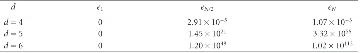
Table 4.2. Approximate error forExample 4.2withc1=(5−
√
15)/10,c2=1/2,c3=(5 +
√ 15)/10.
d e1 eN/2 eN
d=4 0 2.91×10⁻⁵ 1.07×10⁻³
d=5 0 1.45×10²¹ 3.32×1056
d=6 0 1.20×1048 1.02×10112
4. Numerical examples
The method is tested using the following two examples in the interval [0, 1] with step size
h=0.05, errors are computed in Tables4.1 and4.2 for various (3,d,p)-methods with
p=3, 4. The following notations will also be used in the presentation:
e1:=yt1 −ut1 , eN/2:=y(0.5)−u(0.5), eN:=y(1)−u(1), (4.1)
whereu∈Sd3+d(m=3) is the approximated solution.
Example 4.1. Consider the following integro-differential equation of third order:
y(3)(t)=
t
0y(s)ds, y(0)=1, y
(0)=2, y(0)=1, (4.2)
with exact solutiony(t)=et+ sint.
Example 4.2. Consider the following fourth-order integro-differential equation:
y(4)(t)=1 +
t
0y(s)ds, y(0)=y
(0)=y(0)=y(3)(0)=1, (4.3)
with exact solutiony(t)=et.
(a) Let us consider the Gauss points as the collocation parameters, that is,c1=(5− √
15)/10,c2=1/2, andc3=(5 +√15)/10, then we have Tables4.1and4.2corresponding to Examples4.1and4.2, respectively.
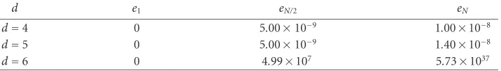
(b) If the first two collocation parameters are the Gauss points, that is,c1=(3−√3)/6,
c2=(3 +√3)/6, andc3=1, then we have Tables4.3and4.4for Examples4.1and4.2. From Tables4.3and4.4, one can observe that (3,d,p)-method (p=3, 4) is stable for
[image:13.468.55.417.188.242.2]Table 4.3. Approximate error forExample 4.1withc1=(3−
√
3)/6,c2=(3 +
√
3)/6,c3=1.
d e1 eN/2 eN
d=3 2.70×10⁻¹⁰ 6.00×10⁻¹⁰ 4.20×10⁻⁹
d=4 2.70×10⁻¹⁰ 4.00×10⁻¹⁰ 5.20×10⁻⁹
d=5 2.70×10⁻¹⁰ 3.95×10¹⁰ 4.53×1040
Table 4.4. Approximate error forExample 4.2withc1=(3−√3)/6,c2=(3 +√3)/6,c3=1.
d e1 eN/2 eN
d=4 0 5.00×10⁻⁹ 1.00×10⁻⁸
d=5 0 5.00×10⁻⁹ 1.40×10⁻⁸
d=6 0 4.99×10⁷ 5.73×1037
andc3=1 as in case (b), and unstable if the collocation parameters are the Gauss points, that is,c1=(5−√15)/10,c2=1/2, andc3=(5 +√15)/10 as in case (a).
References
[1] H. Brunner,A survey of recent advances in the numerical treatment of Volterra integral and integro-differential equations, J. Comput. Appl. Math.8(1982), no. 3, 213–229.
[2] ,Implicit Runge-Kutta methods of optimal order for Volterra integro-differential equa-tions, Math. Comp.42(1984), no. 165, 95–109.
[3] ,The approximate solution of initial-value problems for general Volterra integro-differen-tial equations, Computing40(1988), no. 2, 125–137.
[4] H. Brunner and J. D. Lambert,Stability of numerical methods for Volterra integro-differential equations, Computing (Arch. Elektron. Rechnen)12(1974), no. 1, 75–89.
[5] H. Brunner, A. Pedas, and G. Vainikko,Piecewise polynomial collocation methods for linear Volterra integro-differential equations with weakly singular kernels, SIAM J. Numer. Anal. 39(2001), no. 3, 957–982.
[6] H. Brunner and P. J. van der Houwen,The Numerical Solution of Volterra Equations, CWI Monographs, vol. 3, North-Holland, Amsterdam, 1986.
[7] T. A. Burton,Volterra Integral and Differential Equations, Mathematics in Science and Engi-neering, vol. 167, Academic Press, Florida, 1983.
[8] I. Danciu,Polynomial spline collocation methods for Volterra integro-differential equations, Rev. Anal. Num´er. Th´eor. Approx.25(1996), no. 1-2, 77–91.
[9] , Numerical stability of collocation methods for Volterra integro-differential equations, Rev. Anal. Num´er. Th´eor. Approx.26(1997), no. 1-2, 59–74.
[10] A. Goldfine,Taylor series methods for the solution of Volterra integral and integro-differential equations, Math. Comp.31(1977), no. 139, 691–707.
[11] T. Lin, Y. Lin, M. Rao, and S. Zhang, Petrov-Galerkin methods for linear Volterra integro-differential equations, SIAM J. Numer. Anal.38(2000), no. 3, 937–963.
[12] F. R. Loscalzo,An introduction to the application of spline functions to initial value problems, The-ory and Applications of Spline Functions (Proceedings of Seminar, Math. Research Center, Univ. of Wisconsin, Madison, Wis., 1968) (T. N. E. Greville, ed.), Academic Press, New York, 1969, pp. 37–64.
[image:14.468.58.416.183.234.2][14] R. C. MacCamy,A model for one-dimensional, nonlinear viscoelasticity, Quart. Appl. Math.35 (1977/78), no. 1, 21–33.
[15] ,An integro-differential equation with application in heat flow, Quart. Appl. Math.35 (1977/78), no. 1, 1–19.
[16] G. Micula,Approximate solution of the differential equationy=f(x,y)with spline functions, Math. Comp.27(1973), 807–816.
[17] M. Micul´a and G. Micula,Sur la r´esolution num´erique des ´equations int´egrales du type de Volterra de seconde esp`ece `a l’aide des fonctions splines, Studia Univ. Babes¸-Bolyai Ser. Math.-Mech. 18(1973), no. 2, 65–68 (French).
[18] V. Volterra,Theory of Functionals and of Integral and Integro-Differential Equations, Dover, New York, 1959.
Edris Rawashdeh: Department of Mathematics, Center for Applied Mathematics and Polymer Fluid Dynamics, Central Michigan University, Mt. Pleasant, MI 48859, USA
E-mail address:[email protected]
Dave McDowell: Department of Mathematics, Center for Applied Mathematics and Polymer Fluid Dynamics, Central Michigan University, Mt. Pleasant, MI 48859, USA
E-mail address:[email protected]
Leela Rakesh: Department of Mathematics, Center for Applied Mathematics and Polymer Fluid Dynamics, Central Michigan University, Mt. Pleasant, MI 48859, USA