DESIGN OF EFFICIENT CACHING ALGORITHMS FOR PEER TO PEER NETWORKS TO REDUCE TRAFFIC IN INTERNET

414

SPATIO-TEMPORAL SEGMENTATION AND

CLASSIFICATION ON AERIAL DATA

Mr.K.PRAGADEESWARAN1, Dr.A.SUBRAMANI2 1

Research Scholar, Part Time Category B, Bharathiar University, Coimbatore, Tamilnadu, India.

[email protected]

2

Professor and Head,

Department of Computer

K.S.R. College of Engineering, [email protected]

Tiruchengode, Tamilnadu, India

.

E-mail:

[email protected] ,

[email protected]

ABSTRACT

Classification is one of the standard problems in data mining with a set of training data. Each set has data points and being signified by a feature vector, the significant task to be performed is to algorithmically build a model that measures the class label of an unseen test attribute based on the attribute feature vector. Adaptive Cluster Distance Bounding for High-Dimensional Indexing based on separating hyper plane boundaries of Voronoi clusters develops inter-dimensional correlations. Indexing real high-dimensional data sets focus on the clustering paradigm for search and retrieval but overlapping occurs while using the features of temporal and spatio-temporal data on aerial types of data. The goal is to develop a method which segment the heterogeneous data points in a significant manner, spatiotemporally localize instances of activities in a sequence way and remove overlapping using the seeds. To start with, initially the focal point is obtained by classifying the temporal data using the Spatial-Temporal Segmentation Modeling (SSM) method. SSM then uses individual feature as a seed in order to expand the spatiotemporal specificity on aerial data. SSM ensembles by sampling individual features as seeds by subsequently taking into account their nearest neighbors and further segments heterogeneity data points correspondences according to the coherence value. Finally, the points having significant degree of overlap is discarded that overlap with the temporal and spatio-temporal data. With this lenses dataset extracted from UCI repository, SSM compute the features that are related to spatiotemporal configuration between the training and test sets. Experiments conducted prove the effectiveness of the method and it further shows that the proposed spatio-temporal segmentation algorithm leverages the classification pattern to reduce the average execution time by

increasing the micro averaged accuracy efficiently and effectively

.

Keywords

:

Data Points, Degree of overlap, Coherence.

1. STATE OF ART

Data classification is one of the important topics in the field of data mining due to its extensive applications. A number of related methods have been provided based on the well-known learning models. Even though data

classification was widely conferred,

comparatively few studies explored the

conceptual model of temporal data classification. Most of the existing researches focused on improving the accuracy of classification using arithmetic models, neural network, or distance-based methods.

PaDSkyline for parallel skyline query processing in the middle of partitioned site groups [2] made use of intra group optimization and multi filtering technique to enhance the skyline query processes within every group. In particular, multiple (local) skyline points are sent together with the query as filtering points, which help to identify unqualified local skyline points early on a data site. The mechanism further allocates every unlabeled data points in [9] to match suitable cluster. The novel categorical model using MAximal Resemblance Data Labeling represents clusters by the combinations of attribute values.

Derived membership functions in [3] explain accurately the real distribution of the training data. Besides, the user need not identify the number of extracted features in advance, and trial-and-error for determining the suitable number of extracted features is then avoided. Decision trees for uncertain data in [7] discover that the accuracy of a decision tree classifier are much enhanced if the absolute information of a data item captivating into account the probability density function (pdf)) is utilized. Uncertain data extend classical decision tree building algorithms to hold data tuples with uncertain values.

Among the rich data mining problems, classification modeling and prediction is the significant one due to the involvement of spatio-temporal data such as web attack discovery, customer grouping, and disease diagnosis. Numerous classification methods have been presented including the most significant ones that include decision tree, neural network, support vector machine, and others. The goal of the classification method is to enlarge a model that connects the attribute values to the label for data instances. Hence, the label of a new data instance is predicted properly by using the developed model.

Most of the existing attribute based classifiers on heterogeneity data points expand the model depending on the uniqueness of each data attribute. However, a small portion of studies that discover the issue of incorporated data mining methods to categorize aerial datasets with time sequences, e.g., the time series gene expression datasets were presented. Therefore, they cannot have a high-quality fit on the general temporal dataset classification.

Novel weighted accord function supported by clustering validation criteria [5] initially partitions the candidate items from different perspectives. It introduces an agreement function to add and

reconcile those candidate consensus partitions to a final partition. Novel semi supervised text clustering algorithm, called Seeds Affinity Propagation (SAP) includes two phases namely the new similarity metric that captures the structural information of texts, and a narrative seed construction method to obtain semi supervised clustering process [6].

Along these lines, different types of periodic patterns as shown in [18] work on a suitable transform to reduce the runtime of the algorithm. The ideas of dense periodic regions and minimum period size calculated are also useful and not incorporated to further improve the performance of the algorithm. A thorough investigation of the more sophisticated database backlog estimation approach support quick convergence to the desired performance without introducing extreme delay oscillations in [19].

Global voting algorithm was performed in [21], based on local density and trajectory similarity information for each segment of the trajectory, forms a local trajectory descriptor that represents line segment representativeness. The applicability of the method for (sub) trajectory clustering does not provide concurrently with MOD sampling to hold each sub trajectory of the sampling set. Different sub trajectories of the MOD (cluster) minimize the objective function.

Document Vector Model (DVM) is efficient in constructing the results with high cluster quality. A connection measure is based upon the inferred information during topic maps data and structures. The optional method is implemented using

agglomerative hierarchal clustering and

experimented on standard Information retrieval

(IR) datasets [8]. Hierarchical clustering

algorithm using closed frequent item sets use Wikipedia as external information to improve the document depiction. These ideas are not

comprehensive to additional models like

evolutionary clustering, data streams, etc by using incremental normal item sets in [10]. Cluster-based Temporal Mobile Sequential Pattern Mine (CTMSP-Mine) as presented in [11] discovers the

Cluster-based Temporal Mobile Sequential

Patterns (CTMSPs). Moreover, a forecast strategy was provided to predict the subsequent mobile behaviors.

The heterogeneous documents were

416 semantics. Document Clustering Approaches presented in [14] was based on classification of large data sets that uses the user search Information with fewer keywords using the Internet. Document Clustering play key role for information searching procedure with the help of the user. Text document clustering algorithm TDSCAN (Text Document Structural Clustering of Applications with Noise) requires no previous awareness on the number of clusters as shown in [17]. The algorithm competently makes out outliers, and provides a distribution over possible cluster labels for multi-topical documents based on neighborhood similarity.

Document concepts which were reliable as shown in [15] have manifold geometry such that each concept corresponds to an associated component. The approach was based on the graph model that captures the local geometry of the document sub manifold. The fast minimum

spanning tree-inspired clustering algorithm

presented in [13] uses the significant

implementation of the cut and the cycle property of the smallest amount spanning trees. The rich properties of the existing MST algorithms fails to adapt MST inspired clustering algorithm to more general and larger data sets, particularly when the whole data set cannot fit into the main memory. Expected distances (EDs) between objects and cluster representatives presented in [20] were evaluated using the numerical integrations, which perform costly operations.

Although certain amount of studies was conduct on categorization modeling, reasonably few researches explored the topic of temporal data classification. The existing spatio-temporal data classification methods were normally based on statistical methods, neural networks, or similarity-based techniques. They focused on structure classifiers with high accuracy; however, they were in need of understandable classification rules [1]. In fact, in many applications, there exists a strong need for readable categorization rules in order to appreciate the inherent characteristics of the classifications.

Based on the aforementioned techniques, the proposal presents the classification of features via spatio-temporal segmentation model (SSM) on aerial data. Some of the contributions of SSM include the classification being performed on the temporal data using the Spatial-Temporal Segmentation Modeling (SSM). Next, with the formation of a spatiotemporal shape model which allow to further proceed with localization both in

terms of space and time. Moreover, SSM use feature collections in the proposed model, instead of single features in order to expand the

spatiotemporal specificity on aerial data.

Additionally using SSM, the weighting scheme used to collect all the features that are informative (i.e., they are characteristic of the action) are favored, while votes from collections are commonly activated on temporal and spatio temporal data.

SSM ensembles by sampling individual features as seeds and subsequently taking into account their nearest neighbors and segments

heterogeneity data points correspondences

according to the coherence. Finally, SSM discard the points that have a significant degree of overlap with the temporal and spatio-temporal data using lenses dataset extracted from UCI repository used to compute the micro averaged accuracy, execution time, classification rate, objective function value, segmentation error rate on test datasets and scalability based on degree of overlap removal.

The rest of the paper is planned as follows. Section 2 describes about the different existing work with their confines. Section 3 develops a Spatial-Temporal Segmentation Modeling to remove the degree of overlapping on temporal and spatio-temporal data. Section 4 presents the effective results on the performance parameter using JAVA Weka tool. Section 5 evaluated the

performance and denoted the percentage

improvement with the help of the table and graph values. The final section summarizes a beneficial result with the removal of degree overlapping using seeds and subsequently takes into account the nearest neighbor.

2. SPATIO-TEMPORAL SEGMENTATION MODELING ON AERIAL DATA

and collect that features together for further processing in the subsequent phase.

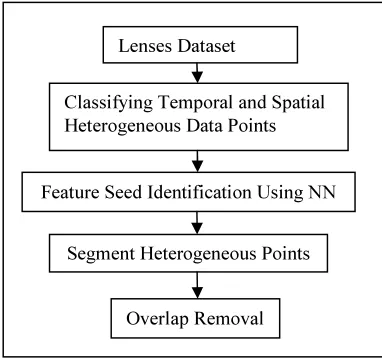
The third phase in SSM segments the heterogeneous data that correspond with the coherence and relations. Segmentation on heterogeneous point is performed using spatio-temporal segmentation method. During the final phase significant degree of overlapping is removed with seeds, such that the redundancy of information is explicit. The architecture diagram including the four phases involved in Spatial-Temporal Segmentation Modeling (SSM) method is shown in Fig2.1.

Fig. 2.1 : Architecture diagram of SSM method

Fig 2.1 describes classifying the temporal data and then use individual feature as a seed in order to expand the spatiotemporal specificity on aerial data. SSM collects all the features as seeds and consequently take into account their nearest neighbors. Next step, segments heterogeneity data points correspondences according to coherence. Finally, it discards the points that have a significant degree of overlap with the temporal and spatio-temporal data. With this lenses dataset, it computes the sets of features that are related to spatiotemporal configuration between the datasets. The forthcoming section discusses in detail about the four phases included in SSM.

2.1 Classifying Temporal and Spatial Heterogeneous Points

The first phase in SSM if the process of classification from heterogeneous data points that

consists of microarray data. Classifying

heterogeneous points produced good result when support vector machine function with the feature

space. The set of temporal and spatial heterogeneous points are non-linearly mapped to higher order feature space by using the particle product operation. Every positive semi definite data function corresponds to the particle product operation in certain higher-dimensional feature space. In SSM work, it constructs a clearly heterogeneous data function by calculating each data type independently and summing the results.

The resulting temporal data uses the prior knowledge about the heterogeneity of the data by accounting higher-order correlations along with features of individual data type. At the same time, the temporal data ignores the higher order correlations across the different data types. With this, the heterogeneous data leads to enhanced performance with respect to support vector machine on the concatenated data. The preceding information of heterogeneity is subjugated when choosing subsets of input features using the classification process.

For most of the temporal based classifications investigated, one type of genomic data provides significantly better training data than the other type. Feature selection algorithms are available for automatically selecting the most useful features for training a classifier whereas the support vector machine method described different types of data point at once, making an exact prediction to each functional category. Indeed, the performance of support vector machine is improved when data types are combined and a single hypothesis is obtained. The combination of two independent hypotheses leads to the wide range of classification.

The experimental evaluation of classification in SSM is performed using cross validation process on spatial, temporal and spatio-temporal data. For a given class, the positively labeled and negatively labeled data are split randomly into ‘n’ groups for cross validation. A support vector machine is trained on n-1 of the groups and is tested on the remaining group. The procedure is repeated ‘n’ times, each time using a different group of as a test set using three fold cross-validations (i.e.) spatial, temporal, and spatio-temporal with n equal to the total number of training examples.

The performance of each support vector machine is measured by investigating how well the classifier identifies the true and false results in the test sets. To judge with the overall performance of classification, the cost factor for using the SSM is defined as provided below.

Lenses Dataset

Classifying Temporal and Spatial Heterogeneous Data Points

Feature Seed Identification Using NN

Segment Heterogeneous Points

418 Cost (SSM Classification) = (spatial(SSM

Classification) + 2temporal(SSM

Classification))/n ……… Eqn (1)

Where, spatial (SSM Classification) represent the number of false result for the classification of spatial points and 2temporal (SSM Classification) denotes the true result for the classification of temporal points in SSM, and n is the number of data points in the class. The true results are weighted more heavily than the false results because, for these data, the number of positive examples is large (i.e.) multiples of 2 compared to the number of negatives.

2.2 Identification of Feature Seeds Using Nearest Neighbor

The second phase involved in SSM is the identification of feature seeds using nearest neighbor. The features that use in SSM classification consist of a grouping of visual stream and temporal gradient descriptors, extracted in the order of detected spatiotemporal data points. However, the SSM are utilized with any kind of local identifiers in order to achieve robustness to detect the data points on the filtered version of the visual stream field. In order to compensate with the filtered version of the visual stream field, more specifically, the median of the visual stream is subtracted with a small spatial window.

Let us denote with the set of visual stream vectors that lie within a cylindrical neighborhood of scale, and centered at location of the action. The location compensated visual stream field of the input data sequence, denote the spatial and temporal level of the neighborhood data. In order to detect data points, initially calculate the signal

entropy GD (l1,l2) within the neighborhood points

NP (l1,l2)

……… Eqn (2)

Where, Qs (p, l1, l2) is the probability solidity of the of level and location function. The set of all signal values are compensated and the optical flow vectors as the signal values. Histogram method approximates the probability solidity and SSM classification collects the spatiotemporal features instead of single features in order to increase the spatiotemporal specificity. By doing so, sets of features that have equivalent

spatiotemporal configuration among the training and test sets are matched. It collects the sampling individual features as seeds by subsequently taking into account their n-1 nearest neighbors.

Gd is the collection of database consisting of ‘SSM classification’ features, where G is the spatiotemporal midpoint for the collections respectively. The identified vector and the spatiotemporal location of the feature identify the similarity between collections. More specifically, the joint probability between the databases Gd is

collected and query collection cq proportional to

………. Eqn (3)

The first term expresses the similarity in the topology of the collections, and the second term expresses the similarity in their values identified. Consequently, each feature of the collection Gd is matched with the feature of the collection cq to identify the maximum similarity in identifier value and relative position within the ensemble. The main goal of SSM is to extract the feature as seed to select feature collections that results in high probability in the true case and with low probability in the false values.

2.3 Segmentation on Heterogeneous Points

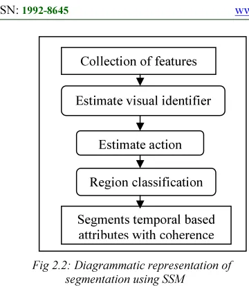
Fig 2.2: Diagrammatic representation of segmentation using SSM

The diagrammatic form of segmentation using SSM provides the necessary information for locating corresponding regions as shown in Fig 2.2. The new location for each region is predicted by giving the previously estimated action for that region. The action models in SSM are estimated within each of these predicted regions and an updated set of action hypotheses derived. Alternatively, the action models estimated from the previous segmentation used by the region classifier directly determine the corresponding coherent action regions. Thus, segmentation based on action conveniently provides a way to track coherent or relation action regions. In addition, when the analysis is initialized with the segmentation, SSM results in the effective robustness of estimation

2.4 Overlap Removal in SSM

Finally, the last phase involved in SSM is the removal of overlap. Spatiotemporal segmentation is not purely a symbol where data is partition into a set of overlapping associated regions. Rather, to have a non-overlap of data in SSM similar action regions are grouped together and represented by a single layer. Thus, even when a single coherent action surface is separated by an occluding foreground surface, these disconnected regions are represented by a single global action model. The SSM data points have an important degree of overlap with the seed on heterogeneous environment. During the implementation of SSM, two points have a significant degree of non-overlap if their normalized distance with respect to their spatiotemporal scale is smaller than a specific threshold.

The algorithm given below assume that a single dominant action are estimated at each iteration, thus, justifying the use of a global action estimator that determine only one action for the entire aerial data.

The algorithm is described below

Begin

Input: ‘n’ Heterogamous data points in lenses dataset, l1-levels and l2-location of data points,

c-collection of features, NP- Neighborhood Points,

Gd - Single Entropy,

Output: Temporal Data Classifier with non-overlapping with seeds

Classification of Temporal Data

1: Classify ‘n’ points with Support Vector Machine

2:Non-lines mappingHigh Order Feature Space

3: Cross Validation process on spatial, temporal and Spatio-temporal data points

4: Cost (SSM) = (Spatial (SSM) +2Temporal (SSM))/n

// Individual Feature Classifier

5: SSM classifier group visual stream of data points

6: Calculate the signal entropy GD (l1, l2)within

the neighborhood points NP (l1, l2)

7: Search n-1 nearest neighbors, individual features represent as seed

8: individual features are collected in Cd

// Heterogeneous Point Segmentation

9: Estimate the visual identifier from collection of features

10: Action estimation locate corresponding region of temporal data

11:Region classifier directly determine the corresponding coherent action regions

12: Segmented temporal data with overlapping points

// Degree of Overlap Removal

13: Compute Normalized Distance

14: Spatiotemporal scale < Specific Threshold Value

15: Removal of Overlapping points on temporal data

End

Upon determining the dominant action, the first attribute is action compensated and compared with the second attribute. The corresponding action region consists of the locations where the errors are small. Recursively, the procedure is applied to the remaining portions of the data points to identify the different action regions. However, estimation of a dominant global action Collection of features

Estimate visual identifier

Estimate action

Region classification

420 inevitably incorporate action from multiple data points producing an intermediate action to estimate with reasonable corresponding action region.

3. PARAMETRIC DEFINITION OF SPATIO-TEMPORAL SEGMENTATION MODELING

Spatio-temporal Segmentation Modeling (SSM) provides efficient outcome after numerous experiments that have been processed on JAVA using Weka tool. SSM uses the Lenses Data Set from UCI repository which are complete and noise free. Lenses dataset is complete with all possible combinations of attribute-value pairs represented. Each instance is complete and correct where 9 rules cover the training set. 3 classes of attribute information are the patient should be fitted with hard contact lenses, the patient should be fitted with soft contact lenses, and the patient should not be fitted with contact lenses.

The 9 complete rules in lenses dataset are

young, pre-presbyopic, presbyopic, myope,

hypermetrope, astigmatic no, astigmatic yes, tear production rate reduced, and normal. Micro averaged accuracy is needy on how data (i.e.) information is collected, and is usually judged by comparing numerous capacity from the same or different sources in heterogeneous points using the Spatial-Temporal Segmentation Modeling. Average execution time is the amount of time taken to perform the classification process on SSM method, measured in terms of seconds (sec).

Average Execution Time= Total time taken for performing classification-Time taken after request send

Classification rate is rate at which effectively performs the classifying of spatial, temporal and spatio-temporal data from the heterogonous points, measured in terms of percentage (%). The Objective Function value of SSM is bounded by numerals from zero. The updating rules for minimizing the objective function of SSM are

essentially iterative. SSM provides better

representation in sense of aerial form of data structure using weka tool.

Scalability is ability of a heterogeneous data points to handle growing amount of work in a capable manner to accommodate the growth based on overlap removal. It refers to the ability of a system to increase total throughput under an

increased load on the temporal data points. Segmentation error rate is defined as the amount of error that occurs on the temporal and

spatio-temporal data segmentation process.

Segmentation process uses the visual identifier estimation for efficient processing where error rate is measured in terms of percentage (%).

4.PERFORMANCE OF SPATIO-TEMPORAL SEGMENTATION MODELING ON AERIAL DATA

The performance of the proposed Spatial-Temporal Segmentation Modeling (SSM) is compared against the existing Adaptive Cluster

Distance Bounding for High-Dimensional

Indexing (ACDB) model. The below table and graph describes the performance on the lenses dataset with the 9 complete rules.

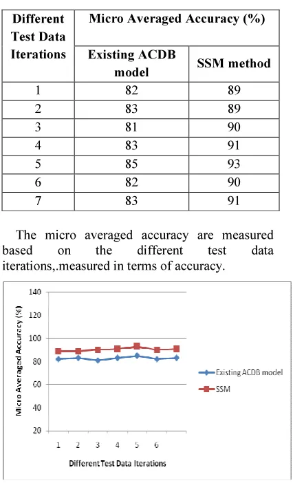
Table 4.1: Tabulation of Micro Averaged Accuracy

Different Test Data Iterations

Micro Averaged Accuracy (%)

Existing ACDB

model SSM method

1 82 89

2 83 89

3 81 90

4 83 91

5 85 93

6 82 90

7 83 91

The micro averaged accuracy are measured

based on the different test data

iterations,.measured in terms of accuracy.

Fig 4.1: Measurement of Micro Averaged Accuracy

points taken from the lenses dataset is used to compute the accuracy rate. The micro averaged accuracy of the SSM method is 5 – 10 % improved when compared with the existing ACDB model by using the multiple activities in heterogeneous data points to obtain result as well as it removes the degree of overlapping with seeds.

Table 4.2: Tabulation of Average Execution Time

No. of distance Computation

Average Execution Time (sec)

Existing ACDB

model SSM

2 75 70

4 120 112

6 164 155

8 192 180

10 250 234

12 325 310

14 410 380

The average execution time taken in existing ACDB model and SSM is tabulated in table 4.2. Execution time are plotted based on the distance is consumes to perform the process.

Fig 4.2: Measure of Average Execution Time

Fig 4.2 explains the execution time based on the distance computation. Distance are measured in meters and it ranges from the 2, 4, 6…14. Execution time taken is 4 – 8 % improved in SSM when compared with the existing ACDB model. The execution time obtained is lesser using SSM because the use of nearest neighbor processing in SSM easily identify the features and collect that features together for further processing in the subsequent phase.

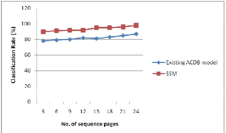
Table 4.3:Tabulation of Classification Rate

No. of sequence

pages

Classification Rate (%) Existing

ACDB model

SSM

3 78 90

6 79 91

9 80 92

12 82 92

15 81 95

18 83 95

21 85 96

24 87 98

Table 4.3 describes the classification rate based on the sequential pages. Sequential pages taken for the evaluation are from 3,6,9,12…24. As the sequential pages increase, classification rate percentage is improved.

Fig 4.3: Measure of Classification Rate

Fig 4.3 describes the classification rate based on sequential pages. Classification rate percentage varies for the different types of sequential pages. Classification rate is 10 – 15 % improved in SSM when compared with the ACDB model. The set of points are non-linearly mapped to a higher order feature space by replacing the particle product

operation for the effective classification.

422

Table 4.4 :Tabulation of Objective Function value

Iterations

Objective Function value Existing

ACDB model

SSM

10 77 75

20 80 77

30 82 79

40 84 80

50 85 82

60 86 83

70 87 85

Fig 4.4: Measure of Objective Function value

Table 4.4 and Fig 4.4 describe objective value function of the SSM and ACDB model. The objective value is decreased to 2 – 5 % in SSM method due to the location compensated visual stream field of the input data sequence that denote the spatial and temporal level of the neighborhood data. Objective value of SSM method is less when compared with the ACDB model, measured against the iteration ranging from 10, 20,…70.

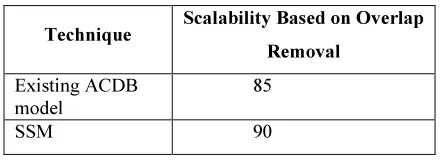
Table 4.5: Tabulation of Scalability based on overlap removal

Scalability of ACDB model and SSM method is plotted in table and graph to show the efficiency.

Fig 4.5 :Measure of Scalability based on overlap Removal

Measure of scalability in SSM based on overlap removal is approximately 5 % improved in SSM because of using the significant degree of overlap with two points. This is because the two points have a significant degree of non-overlap as the normalized distance with respect to their spatiotemporal scale is smaller than a specific threshold, measured and depicted in terms of percentage value.

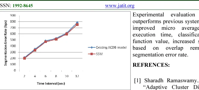
Table 4.6: Tabulation of Segmentation Error Rate

Time Interval (sec)

Segmentation Error Rate (bps)

Existing

ACDB model SSM

2 213 201

4 350 334

6 485 471

8 526 513

10 614 598

12 784 753

Segmentation error rate are measured based on the time interval and shown in Table 4.6. Time interval point varies from 2, 4, 6,…12 seconds. Error rate graph points are plotted to these time interval.

Technique Scalability Based on Overlap Removal

Existing ACDB model

85

Fig 4.6 :Measure of Segmentation Error Rate

Fig 4.6 describes the segmentation error rate on SSM and ACDB model. As the time interval range varies, error rate is also decreased gradually. The error rate measured in terms of bits per second reduces in SSM from 2 – 6 % when compared with the ACDB model.SSM error rate is decreased using the region classifier that directly determine the corresponding coherent action regions, so that the errors are minimized.

As the final point, it is being observed that the SSM efficiently process the four phases, with the non-overlapping form of heterogeneous data points. In order to improve the accuracy rate of SSM, research focus has been shifted from

designing model to relate the sets of

spatiotemporal configuration features between the training and test sets.

5. CONCLUSION

Spatial-Temporal Segmentation Modeling

(SSM) with support vector machine allows direct comparison across different feature combinations. Support vector machine classify a larger class of data points for gaining the popularity. SSM then use individual feature as a seed in order to expand the spatiotemporal specificity on aerial data.

Once the classification process being

accomplished in SSM, algorithm allows for competing between different actions hypotheses to in order to produce multiple distinct action regions. These action regions at iteration segment the temporal data points. Temporal segmentation is achieved by tracking the action regions that uses the affine motion model to segment the action data. The segmentation provides the necessary information to derive the depiction whereby data is reduce to few layers (i.e.) only

temporal data, corresponding to temporal

coherences of the data. Finally non-overlapping form of data points is obtained through SSM.

Experimental evaluation is conducted and outperforms previous systems in terms of 7.714% improved micro averaged accuracy, lesser execution time, classification rate, objective function value, increased scalability assessment

based on overlap removal and minimal

segmentation error rate.

REFRENCES:

[1] Sharadh Ramaswamy., and Kenneth Rose., “Adaptive Cluster Distance Bounding for

High-Dimensional Indexing,” IEEE

TRANSACTIONS ON KNOWLEDGE AND DATA ENGINEERING, vol. 23, no. 6, june 2011.

[2] Lijiang Chen., Bin Cui., and Hua Lu.,

“Constrained Skyline Query Processing

against Distributed Data Sites,” IEEE

TRANSACTIONS ON KNOWLEDGE AND

DATA ENGINEERING, vol. 23, no. 2,

february 2011.

[3] Jung-Yi Jiang., Ren-Jia Liou., and Shie-Jue Lee., “A Fuzzy Self-Constructing Feature Clustering Algorithm for Text Classification,” IEEE TRANSACTIONS ON KNOWLEDGE AND DATA ENGINEERING, vol. 23, no. 3, march 2011 .

[4] Ninad Thakoor., and Jean Gao.,

“Branch-and-Bound for Model Selection and Its

Computational Complexity,” IEEE

TRANSACTIONS ON KNOWLEDGE AND DATA ENGINEERING, vol. 23, no. 5, may 2011.

[5] Yun Yang., and Ke Chen., “Temporal Data Clustering via Weighted Clustering Ensemble

with Different Representations,” IEEE

TRANSACTIONS ON KNOWLEDGE AND DATA ENGINEERING, vol. 23, no. 2, february 2011.

[6] Renchu Guan., Xiaohu Shi., Maurizio Marchese., Chen Yang., and Yanchun Liang.,

“Text Clustering with Seeds Affinity

Propagation,” IEEE TRANSACTIONS ON

KNOWLEDGE AND DATA

ENGINEERING, vol. 23, no. 4, april 2011. [7] Smith Tsang., Ben Kao., Kevin Y. Yip.,

Wai-Shing Ho., and Sau Dan Lee., “Decision Trees for Uncertain Data,” IEEE TRANSACTIONS

ON KNOWLEDGE AND DATA

424 Computer Applications (0975 – 8887) Volume 12– No.1, 2010.

[9] Hung-Leng Chen., Ming-Syan Chen., and

Su-Chen Lin., “Catching the Trend: A

Framework for Clustering Concept-Drifting Categorical Data,” IEEE TRANSACTIONS

ON KNOWLEDGE AND DATA

ENGINEERING, vol. 21, no. 5, may 2009. [10] Kiran G V R., Ravi Shankar., and Vikram

Pudi., “Frequent Item set Based Hierarchical Document Clustering Using Wikipedia as External Knowledge,” springer-verlag berlin heidelberg 2010.

[11] Eric Hsueh-Chan Lu., Vincent S. Tseng., and

Philip S. Yu., “Mining Cluster-Based

Temporal Mobile Sequential Patterns in Location-Based Service Environments,” IEEE TRANSACTIONS ON KNOWLEDGE AND DATA ENGINEERING, vol. 23, no. 6, june 2011.

[12]K.Sathiyakumari.,G.Manimekalai.,

V.Preamsudha., “A Survey on Various

Approaches in Document Clustering.,”

International Journal Computer Technology Vol 2 (5), 1534-1539, 2011.

[13] Xiaochun Wang, Xiali Wang, and D. Mitchell Wilkes., “A Divide-and-Conquer Approach for Minimum Spanning Tree-Based Clustering,” IEEE TRANSACTIONS ON

KNOWLEDGE AND DATA

ENGINEERING, vol. 21, no. 7, july 2009. [14] Swatantra kumar sahu., Neeraj Sahu.,

G.S.Thakur., “Classification of Document Clustering Approaches,” International Journal of Advanced Research in Computer Science and Software Engineering, Volume 2, Issue 5, May 2012 ISSN: 2277, 2012.

[15] Deng Cai., Xiaofei He., and Jiawei Han., “Locally Consistent Concept Factorization for

Document Clustering,” IEEE

TRANSACTIONS ON KNOWLEDGE AND DATA ENGINEERING, vol. 23, no. 6, june 2011.

[16] Duc Thang Nguyen., Lihui Chen., and Chee

Keong Chan., “Clustering with Multi

viewpoint-Based Similarity Measure,” IEEE TRANSACTIONS ON KNOWLEDGE AND DATA ENGINEERING, vol. 24, no. 6, june 2012.

[17] Xun Li., “TDSCAN: A Density Based Algorithm for Text Documents Clustering,” International journal on text clustering, 2011. [18] Faraz Rasheed., Mohammed Alshalalfa., Reda

Alhajj., “Efficient Periodicity Mining in Time

Series Databases Using Suffix Trees,” IEEE TRANSACTIONS ON KNOWLEDGE AND DATA ENGINEERING., 2010

[19] Kyoung-Don Kang., Yan Zhou., and Jisu Oh., “Estimating and Enhancing Real-Time Data

Service Delays: Control-Theoretic

Approaches,” IEEE TRANSACTIONS ON

KNOWLEDGE AND DATA

ENGINEERING, vol. 23, no. 4, april 2011. [20] Ben Kao., Sau Dan Lee., Foris K.F. Lee.,

David Wai-lok Cheung., and Wai-Shing Ho., “Clustering Uncertain Data Using Voronoi

Diagrams and R-Tree Index,” IEEE

TRANSACTIONS ON KNOWLEDGE AND DATA ENGINEERING, vol. 22, no. 9, september 2010.

[21] Costas Panagiotakis., Nikos Pelekis, Ioannis Kopanakis., Emmanuel Ramasso., and Yannis Theodoridis., “Segmentation and Sampling of

Moving Object Trajectories Based on

Representativeness,” IEEE TRANSACTIONS

ON KNOWLEDGE AND DATA

ENGINEERING, vol. 24, no. 7, july 2012.