Munich Personal RePEc Archive
Human Development in India: Regional
Pattern and Policy Issues
Majumder, Rajarshi
Dept of Economics, University of Burdwan
2004
Online at
https://mpra.ub.uni-muenchen.de/4821/
1
Human Development in India: Regional Pattern and Policy Issues
Rajarshi Majumder
Department of Economics University of Burdwan
Golapbag, Burdwan West Bengal – 713104 Email: [email protected]
Please refer to this article as appearing in Indian
Journal of Applied Economics, Vol. 2, No. 1, 2005
Biographical Details: The author has done his doctoral thesis from Centre for the Study of
Regional Development, Jawaharlal Nehru University, New Delhi. He presently teaches
Economics at University of Burdwan, West Bengal. His areas of interest are Regional
Disparity, Infrastructure, Human Resource, and Energy.
Acknowledgement is due to Prof. Ashok Mathur and Dr. Dipa Mukherjee for their valuable
comments on the first draft. I am grateful to the participants of a seminar at Vidyasagar
Univesity, Midnapore, WB for their comments during a presentation of this topic. Comments
1
Human Development in India: Regional Pattern and Policy Issues
Abstract
Development literature in the past decade has become more people centric with human
development being projected as one of the ‘ends’ of development planning. The present
paper tries to explore the trends, patterns and regional dimension of human development
(HD) in India through construction of alternate HD indices. The association between HD
indices and conventional measures like per capita income has been explored. Substantial
inter-regional disparity in HD is observed. Probable reasons for such disparity have been
inquired. Suggested policies to enhance HD include greater role of the State in
provisioning of social infrastructure, especially to the hitherto marginalized groups.
1. Introduction
Development economics in recent years have become more people centric than before. It has
rediscovered that human beings are both the means and the end of economic development
process, and without Human Development (HD) that process becomes a hollow rhetoric. The
maze of technical concepts and growth centric approach to development ruled the roost for
the most of post war period. Only from the eighties onwards, we started to recognize that
human needs and capabilities are necessary ingredients for success of any growth strategy.
The pioneering work of Mahbub ul Haq and Paul Streeten under the aegis of UNDP finally
institutionalised the importance of HD and the Human Development Reports brought out
annually by UNDP reflects the condition of human being in different parts of the world. It
has come to be recognised that improvements of human beings – their capabilities, skills and
2 over’ effects as greater capabilities lead to higher productivity levels, increased income
levels, and wider scope for further human capital formation. Thus uplifting of a single
generation of citizen propels all future generations on to a higher growth trajectory. The
‘trickle down’ effects also are significant as better living standards lead to greater care for the
environment & resources, a healthy & democratic civic society, and a lower discrimination
based on gender, race and caste. These multiple roles of HD have catapulted it to centre-stage
of research and discussion in recent years. As it has come to stay in limelight for a
considerable time, techniques have been developed to objectively measure levels of HD and
facilitate comparison across space and time.
The importance of HD is much more pronounced in a developing nation like India. Here
development would mean improving the condition of human life – an end in itself – and the
growth of income or spread of industries or the expansion of agriculture are to be seen as
only means towards that end. More than fifty years ago, on an August night, our premier
Prime Minister had called for “the ending of poverty and ignorance and disease and
inequality of opportunity”. These were the ‘tasks’ that faced a nascent nation burdened with
ages of deprivation, inequality and low human standards. After five decades of measuring our
success by the GNP growth, we must go back to those ‘tasks’ that were laid down for us and
examine what we have achieved in reality. In this paper, we make an effort to trace the trend
and regional issues related to human development in India over the period 1971-2001. The
paper is divided into eight sections. In the next section, we discuss the methodology used for
the study. The third section deals with the trends exhibited by HD at the National as well as
Regional level during the period 1971-2001. The fourth and fifth sections analyse those
trends in light of regional disparity in development levels. The sixth and seventh sections
briefly visit some of the correlates and impacts of HD. A short summary as well as Policy
3
2. Methodology
Any study that attempts to study human development, over so vast a space as of India must
be careful about, and give serious thoughts to, two very important aspects. They are: (a)
Choice of variables or indicators, and, (b) The method of combining them into indices.
Both of them must be discussed in some detail.
Conventional indicators of development proper measure the end result of development
process, namely - income generation, capital formation, or sectoral transition. But HD should
include both capabilities in non-economic and economic domain. The general trend has been
to include Health and Education as the two other capabilities that should supplement
purchasing power in measuring HD. This approach has been taken by UNDP and has been
followed by most of the researchers. But if we are to segregate between social capabilities
from economic capabilities and explore how far the former enhances economic benefits, then
the HDI should not include income capabilities. Consequently, in this paper we have
developed two alternate measures of HD – Social Development Index (SDI – reflecting
education and health conditions), and the conventional HDI (which includes income
capability also). However, this is done at the second stage only. At the first stage, indices are
prepared for Educational Development (EDI) and Health/Medical Development (MDI).
Then, SDI is prepared from EDI and MDI while HDI is prepared from EDI, MDI and Per
capita NSDP (PCNSDP).1
The second major methodological issue to be discussed is the method of combining the
indicators to arrive at composite score. After grouping the variables under the
sub-components already discussed, we have to construct composite indices representing EDI,
MDI, SDI and HDI for the states of India, as well as the National level for each of the 30
years. The conventional measure of HDI (and its variants as evolved by various researchers
4 weightage scheme. This method suffers from the problem of value-judgement whereby
education, health and income are given equal weightage in the preparation of HDI. Even
within educational attainment index, literacy and enrolment are combined in pre-fixed ratios.
While the weightage scheme is (and has been) subject to various criticisms, the one that
appeals most is that it does not take into account the real data. A situation where the
observations are similar in educational attainments but disperse in health achievements
should attach more importance to the later compared to the former while combining them so
that the combined index brings out the disparity among the observations up to the maximum
extent possible. This is generally done using Factor Analysis. Factor Analysis tries to find out
the fundamental, or latent, ‘Factor’ within each cluster or group. Thus, each group would be
combined into a ‘factor’ by linear combination of the variables of that group. This factor
captures the essence or profile of that particular group and can then be used as a new variable
representing a particular set of variables, or, in broader terms, a particular aspect of the data.
The most commonly and frequently used method of Factor Analysis nowadays is the
Principal Component (PC) Method.2 This method is considered better than giving weightages
based on individual value-judgement, and is both popular and widely used by researchers.3 A
variant of this PC Method (Modified PC analysis – MODPCA) presumes that variables that
significantly affect spatial spread of facilities have the tendency to be unevenly distributed
over space (and time).4 Consequently, they have high dispersion or variance and must also be
given higher weightages while constructing the composite index. This can be done by finding
out such a composite factor that would maximize the Sum of Squared Projections of the
variables - the variables retaining their variance and not being transformed to have equal
standard deviation through normalization.
In the present study, we accept the reality that variables measuring HD are widely dispersed
5 levels. Consequently, MODPCA is used to construct the composite indices by finding out
such a ' Weight' vector that maximizes the sum of squared projection of the transformed data
matrix - after transforming them by dividing by mean.5
EDI and MDI are thus prepared using the MODPCA method. Index of social development
level is prepared by using MODPCA on the individual indicators of EDI and MDI to give us
SDI. First index of HD (HDI1) is then prepared by using MODPCA on the individual
indicators of EDI & MDI and PCNSDP (PCGDP at national level). HDI2 is prepared by
using the conventional (or revised UNDP) method of weightage. Thus, total 4 indices are
prepared by using MODPCA: EDI, MDI, SDI, and HDI1. The process of combining has been
done using the whole data set, i.e. for 16 States for all the 30 years. This implies that the
standardization has been done using the same scale and the composite scores thus prepared
are comparable among themselves. To derive HD indices for All India, the weight vector
used for the states were used as weights on indicators for India. In almost all cases, the First
Principal Component is able to explain more than 70% of the variation in the data matrix.
Let us then venture into study of HD in India using these indices.
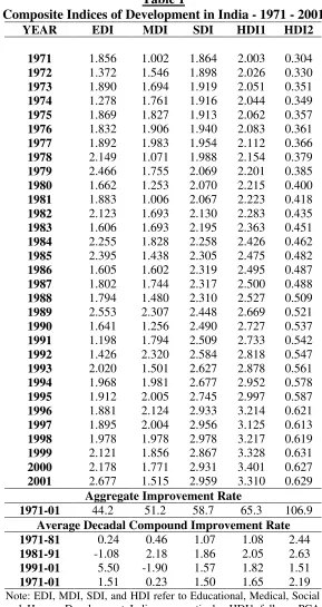
3. Trends in Levels of Human Development in India
There has been a sustained rise in the parameters measuring level of development, both at the
National and at the state level during the 30 years of study. If we look at National data (Table
1), we find that both the components of HD − EDI and HDI have shown a continuous rise
during 1971-2001. The factor scores have increased by greater proportion for EDI compared
to MDI. Consequently, SDI, HDI1 and HDI2 have also shown a sustained rise during this
period. The rise in PCGDP has by far outstripped the social indices, and as a result, rise in
HDI have been greater compared to those related to social sectors only. This indicates that the
6 improvement in human capabilities. This does not augur well for sustainability of the
development process.
However, this rise in HD indicators has not been smooth or stable over the years. We can
segment the study period into 6 quinquenna to examine this trend. Taking three yearly
averages, scores of the indices for the 7 time-points – 1971, 1976, 1981, 1986, 1991, 1996
and 2001 are constructed. These scores are used in subsequent analysis (Table 2). This will
also enable us to explore the post-reform dynamics by studying the 1991-96 and 1996-2001
periods.6
It is observed that EDI increased during the first and the third quinquenna, but declined
during the second and the fourth one. During the ‘90s however, it has improved remarkably.
On the other hand, MDI exhibited a steady rise during the first five periods, but during
1996-2001, it dropped by almost 6% annually. As a result, the improvement rates (since all our
measures except PCNSDP are indices, we refrain from using the term ‘Growth Rate’) of SDI,
HDI1 and HDI2 have been erratic over the six periods, though they have been positive all
through. More or less similar trends are observed for the major states also.
Thus, it can be commented that the period 1971-2001 has experienced a steady improvement
of human development levels in both the nation as a whole and the major states. However,
one has to keep in mind that the improvement seems impressive more because the initial
levels were too low. While it must be accepted that we have come a long way compared to
from where we started, the absolute levels are still not satisfactory, especially if compared to
international standards. For example, over the 30-year period 1971-2001, EDI, MDI, SDI and
HDI1 have increased in India by 45-65 %, and HDI2 have increased by 107%. On the other
7 increased by 225% in Botswana, 160% in China and S. Korea, and over 140% in Malaysia.
The Human Development Report 2003 (UNDP 2003) ranks India at 127 among 175 nations,
just after Morocco and before Ghana, with a score of 0.590, compared to the highest score of
0.944 achieved by Norway. There has been only 42% improvement in HDI over 1975-2001
period in India, compared to 74 per cent in Nepal, more than 49 percent in Egypt &
Bangladesh, and 47 per cent in Indonesia. This matter has to be noted with caution.
4. Regional Disparity in Human Development
One of the major concerns of economic planners in India has been the regional inequality in
the fruits of development. There had been a huge gap between active and vibrant regions and
the hinterland during the pre-independence period in terms of availability of facilities and this
manifested itself in the form of unequal levels of development – both economic and human.
On attaining independence, our proclaimed objective was to bring about regional equality in
growth and development even at the cost of efficiency and aggregate growth. It is necessary
to examine whether that intention has fully materialised.
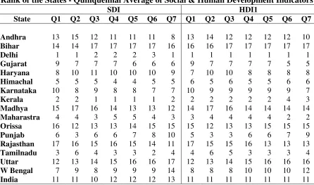
a) Hierarchy of the states
Let us now examine the relative position of the states regarding different development indices
(Table 3a and IIIb). It can be seen that the hierarchy has remained fairly similar over time –
with the same states retaining the top and bottom positions. Delhi captures the top-most
position for all the three development parameters for most of the years. This may have been
caused by simultaneous working of different factors like - its small geographical size, its
importance as the National Capital City and the huge capital expenditure incurred to
modernize, develop and promote the National Capital Territory and make it comparable with
other international cities. Among the other states, Kerala, Maharashtra and Himachal Pradesh
put up consistently good performance regarding social and human development indicators.
8 as indicated by its low PCNSDP rank. On the other hand, Gujarat, in spite of its having low
HD ranks, have consistently good ranking in PCNSDP.
If we look more closely, a regional pattern emerges from the hierarchy of the states. It seems
that the Northern, and Eastern states are persistently doing poorly in terms of HDI, whereas
the Southern states (except Andhra Pradesh) are doing well along with the Western states.
This clearly reflects a regional pattern with the Eastern, Northern and Central regions
performing poorly with only West Bengal reaching close to the national average level of
human development. This regional disparity is of grave concern. The only consolation is that
when we look at the improvement rates, it seems that there is a tendency for the erstwhile
lagging regions to slowly catch up with the other advanced regions of our country, which is
heartening and desired.
b) Regional Disparity and Convergence - Divergence theory
Table 4 shows the inter-state variation in the different indicators of HD for the 1971-2001
period. It is observed that substantial variation exists in the level of HD among the states,
measured by the Coefficient of Variation (CV). The variation is higher in EDI compared to
MDI, and in HDI compared to SDI. This is caused by the relatively higher variation in
PCNSDP compared to the humane indices.
More important than the levels of variation are the trends exhibited by the variation, i.e.
whether the distribution is showing greater equality or otherwise over time. This has been
done in economic literature using the two tests - σ test and β test. The former uses any rise
(or fall) in CV as an indicator of rising (or falling) inequality. The later finds out the
9 positive, β test would conclude that higher initial levels lead to higher growth rate and hence
Divergence in development levels. A negative association would indicate Convergence.
Various researchers have studied the trends in Inter-State variation in economic development
and tried to find out whether the inequalities have widened over time. Many of them have
commented that the pattern has followed the much-discussed ‘Inverted-U’ relatio nship,
whereby the variation (measured mostly by coefficient of variation) has increased during the
immediate period following development efforts (Williamson 1965, 1968). However, as the
development results started to ‘spread’ and ‘trickle down’, the vari ation started to decline.
Others however have refuted the existence of such a relationship in India and have shown
that the relationship is in fact an ‘Upright-U’ one.7 They point out that there had been a
decline in the inter-state differences during the Fifties and the early and middle Sixties, but
thereafter the differences increased noticeably. Let us now investigate this issue for the HD
indices using the present framework (Table 5).
σ test: The experience of the states seems to be somewhat varied, along with an overall
declining trend, if the σ test is used. Disparity in EDI declined consistently during 1971-1996
period but increased during 1996-2001 period. On the other hand, variation in MDI exhibits
an alternate rise-fall cycle. When the composite indices are studied, it is observed that
variation in all the three indicators - SDI, HDI1 and HDI2 - across states declined steadily
during 1971-2001. Only HDI1 has shown a diverging tendency during 1996-2001.
β test: For conducting the β test the average annual improvement rates in each quinquenna
have been regressed on the initial level with the states as observations. It is observed that
EDI, MDI, SDI and HDI1 has shown converging tendencies all throughout (except
divergence in HDI1 during 1971-76 period). Only during the 1991-96 period, i.e. the
10 we find that while during 1976-81 period there was some converging tendencies, diverging
tendencies have been experienced thereafter. During the 1996-2001 period, we can again
trace a hint of stability in regional distribution of PCNSDP.
Broadly speaking, it can thus be concluded that variation in human development indicators
have shown a steadily declining trend. However, the regional disparity seems to have
increased in the immediate post-reform period for HDI1, a major cause of which is further
slowing down of already poorly performing states. In fact, the difference between the average
level of the better-off states and that of the worse-off states have widened during the
immediate post-reform period. Though the situation has been reconciled to some extent in the
next quinquenna, it remains a perennial source of concern.
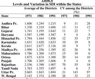
5. Intra-state Variation in Levels of Human Development
It has been so far indicated that inter-state differences in HD is a major characteristic of
development experience in India. Let us come down one further level and look at Intra-state
variations in development. For this purpose, index of human development is prepared for the
Districts of the 16 states for 3 time points - 1971, 1981, and 1991.8 However, due to
non-availability of comparable estimates of domestic products at the district level, we cannot
prepare HDI1 and HDI2 for them. Thus, this part of the analysis is based on District level
scores of SDI. Intra-state variation for a particular state is then measured by the CV obtained
from the district scores of that state while their mean gives the Average level of development.
Table 6 gives the Average level and Coefficient of Variation across districts exhibited by SDI
for the states for the three years.
It can be noted that the state variation is substantially high in many states. Highest
intra-state disparity was observed in Rajasthan in 1971, and in Uttar Pradesh in 1981 and 1991. It
11 itself is low, e.g. Rajasthan, Uttar Pradesh, and Madhya Pradesh. This is of major significance
since one can easily apprehend how far underdeveloped some of the districts in those states
are. This also implies that these states are not only suffering from low average level of human
development, but also that there are only a few isolated pockets of development in those
states while the rest of the districts are lagging far behind. Moreover, it can also be seen that
intra-state variation seems to be low in the advanced states (i.e. states with high average value
of the indicators). This implies that those developed states have managed to improve their
average level not by concentrating on a few isolated regions but by spreading the facilities
more evenly across space. It thus comes out that the inequality is low at the upper end of
development.
To test whether the inequality follows any pattern, especially to check whether the intra-state
variation depends on the average level itself, the mean level and the coefficient of variation
were subjected to Correlation Analysis. It was observed that that the Correlation Coefficients
were small and insignificant and there seems to be no linear association between the average
level and intra-state disparity.
This issue was further investigated with the help of ‘Scatter Plots’ to form an idea about the
nature of the association. A loose Inverted-U shaped relation between the Coefficient of
Variation and the Average level of the States may be inferred. This supports the
often-discussed Kuznets’ hypothesis that the inequality is low at lower ends of development level,
increases as development proceeds, and then again decreases at upper levels of development.
6. Human Development in India – Some Correlates
We may seek to identify various possible correlates of social and human development in
India. This will be helpful in understanding the reasons behind regional dissimilarity in social
12 Development of the social and human standards crucially depends on the infrastructure
available (mostly provided by the State) for social services. Composite indices of educational,
health and aggregate social infrastructure were prepared for an earlier study (Majumder,
2003). It is observed that the levels of HD in the states and districts are significantly positive
associated with these infrastructural availability indices (Table 7). This implies that the
regional disparity in availability of schooling, medical and health facilities are a major reason
behind lopsided social and human development in the states of India. This also underlines the
need for the State to ensure better and more evenly spaced out facilities.
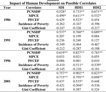
7. Impact of Human Development
What are the most visible impacts of HD? If we consider HD as ‘means’ for attaining ‘ends’,
then the most natural impact of human development would be on economic well being of the
people. We find this to be true. The association between HDI and SDI on one hand, and
economic indicators like PCNSDP, Monthly Private Consumption Expenditure (MPCE),
Private Final Consumption Expenditure on Food (PFCEF) on the other, are observed to be
significantly positive (Table 8). Though the relation with HDI may be questioned on the basis
of circularity (since HDI contains PCNSDP), that between purely non-economic factor SDI
and the economic well being levels is remarkable.
However, one of the major impacts of HD is to make people more capable in a holistic sense.
Improvements in health, education and earning capabilities have greater marginal benefit for
the poor and the excluded. Thus, a rise in overall level of HD is expected to lead to a more
equal distribution of economic opportunities along with the rise in its average level. To
explore this issue, the association of economic inequality (as given by the Gini coefficient of
13 the periods, this association is significantly negative. This indicates that with rising social and
human development levels, one takes long strides in attaining egalitarianism as well.
However, for 2001 the association between HD levels and consumption Gini is observed to
be positive, indicating rising economic inequality in the states with high HD levels. The post
reform changes in structure and nature of capabilities demanded may have caused a
substantial portion of people to be excluded from economic processes even in the developed
states. Given that the inequality among the states (and also that within the states) are quite
substantial even in 2001, this is of serious concern as the benefits of five decades of planned
development may be undermined. The excluded mass of people will become desperate to
snatch the right to acquire capabilities and improve their living standards, and the elite will be
equally desperate to hold on to their privilege. This is a fertile ground for civic unrest and it is
not surprising that the extremist activities in India are emerging in vast tracts of relatively
backward areas like Central Indian plains, Telengana and North-eastern region. This issue
requires greater attention of both academicians and policy makers.
8. Summary Findings and Policy Issues
The major findings can be summarized as:
1. The levels of HD in India and its constituent states have increased substantially during
the three decades of the present study;
2. The improvement rates have been moderate when compared to global experiences;
3. The hierarchical position of the states has remained more or less similar over the period
1971-2001;
4. While educational opportunities have expanded in the post reform period, medical and
health standards have deteriorated in this period;
14 6. Regional disparity seems to have declined over the years but has increased for HDI1 in
the immediate post reform period;
7. The main cause of rising regional disparity in the immediate post reform period has
been the slowing down of the worse-off states and acceleration of the better-off states;
8. This has direct correlation with the withdrawal of the State from provisioning of health
and medical facilities in particular and developmental projects in general;
9. The impact of rising HD levels seems to be not only on the aggregate income and
consumption levels, but also on the incidence of poverty and intra-state consumption
inequality.
What lesson does this hold for policy makers? While the importance of HD is underlined,
India must concentrate on its regional and inter-personal disparity and distributional effects.
Huge diversity among regions and groups of people create serious inequality among people
both across states and within the same state. To resolve these issues, important tools in the
hands of the policy makers seems to be provisioning of social infrastructure. In this era of
withdrawing state support, a few words in this context are worth mentioning. Social
infrastructure provisioning in India has always been burdened with the preconceived notion
that these are not profitable activities and the provisioning of those services has to be the
responsibility of the State. Theoretically, this is justified by the ‘Social Good’ character of
these services and the related External Economies. However, this method is facing increasing
problems because of excess demand, inefficient services, failure of the Government to
upgrade technology and inefficient management. The state has had to shoulder the financial
burden of providing such services, which have become increasingly costly over time. There
has been no effort to recover ‘user charges’ or even any analysis to gauge the prices that the
15 exchequer. As the resource crunch has become serious in recent times, the allocation of funds
to these sectors has slowed down and the State is increasingly unable to meet the rising
demand for such services. But withdrawal of the State affects the poorer section of the people
and not the rich who can afford private purchase of those services. Galbraith’s comment
about ‘Private affluence amid public squalor’ is most appropriate to describe the situation. As
a result, human development is bound to suffer a setback (At the higher ends of human
development levels, availability or otherwise of services does not have much effect as they
are already on the higher HD trajectory. But at the lower ends of the scale, huge marginal
impacts are evident). Consequently, instead of withdrawing its services in blanket terms, the
govt. must adopt a differential price policy. Differential prices must be based on ‘Block
Tariff’ policy, where a subsidized rate is charged for first few units of service (called the
‘lifeline’ rate) so that the poor can access the service, at least up to the basic minimum
necessity level. Beyond that, the rates must be taxed to recoup the subsidy - so that rich or
heavy users pay more than the cost. This will make the services sustainable without
sacrificing the goals of social equity.
In other words, we must sincerely endeavour to create an environment and policy atmosphere
that will uplift and empower the socially marginalized and hitherto excluded mass of people.
The real answer lies in adopting a development model based on ‘equality of opportunity’ and
centrality of human beings, where fixation with growth does not overshadow the real people
for whom growth is advocated. After 50 years, the struggle for independence is still on.
Notes
1
The indicators used to construct the indices are as follows. EDI – Literacy percentage and Gross Enrolment Ratio in Primary, Middle and Secondary stages. MDI – Infant Mortality Rate, Crude Birth Rate and Crude Death Rate (after suitably transforming them to reflect positive dimension).
2
16
3
For a precise analytical study of various methods of construction of composite indices see Kundu, A. (1980) and Kundu and Raza (1982).
4
In the present case however, there is a-priori logic in favour of this method, as we have already alienated the variables in such a way that indicators reflecting a certain aspect of HD are grouped together. Thus, they are likely to move together rather than astray.
5
This MODPCA method has been evolved by Amitabh Kundu et al. Refer to Kundu (1980).
6
It is often argued that the mean used should not be the simple average of the indicators, but an weighted average of them, the weights being either area or population of the observations (districts or states), depending on which factor the indicator was standardized by. However here the purpose is to make the variables scale-free and express them relative to a common factor. Hence simple mean will serve our purpose.
7
Structural Adjustment Programme was initiated in big way in India in 1991 – generally known as the year of reforms. Post-1991 developments generally are referred to as pos-reforms dynamics.
8
Mathur (1983) obtained such U-shaped pattern for the 1950-51 - 1975-76 period in India for Aggregate Per Capita State Income, and also for Per Capita State Income from Primary, and Tertiary sectors. For Secondary sector he obtained an Inverted-U shaped pattern. Other studies include Rao (1973), Sampath (1977), Mohapatra (1978) and Nair (1982).
9
17 References
Chattopadhyaya, B. and Moonis Raza (1975) “Regional Development - An Analytical
Framework and Indicators”, Indian Journal of Regional Science, 7 (1).
Chattopadhyaya, R.N. and M.N. Pal (1972) “Some Comparative Studies on the Composition
of Composite Regional Indices”, Indian Journal of Regional Science, 4 (2).
Chaudhry, M.D. (1974) “Behaviour of Spatial Income Inequality in a Developing Economy:
India, 1950-70”, Paper presented at the Conference of the Indian
Association for Research in National Income and Wealth, New Delhi, 1974.
Das, Tushar K. (1998) “‘Convergence’ and ‘Catc hup’: An empirical Analysis with Fourteen
Major States of India”, Working Paper, Dept. of Analytical and Applied
Economics, Utkal University.
Dhar, P.N. and D.U. Sastry (1969) “Inter-State Variations in Industry, 1951-61”, Economic
and Political Weekly, 4 (12).
Ganguli, B.N. and D.B. Gupta (1976). Levels of Living in India: An Interstate Profile.
(New Delhi, S. Chand).
Gupta, S.P. (1973) “The Role of Public Sector in Reducing Regional Income Disparity in
Indian Plans”, Journal of Development Studies, 9 (2).
Kothari, C.R. (1988). Research Methodology: Methods and Techniques. (New Delhi,
Wiley Eastern Ltd.)
Kundu, Amitabh (1980). Measurement of Urban Process - A Study in Regionalisation.
(Bombay, Popular Publishers)
Kundu, Amitabh and Moonis Raza (1982). Indian Economy - The Regional Dimension.
(New Delhi, Spectrum Publishers)
Lahiri, R.K. (1969) “Some aspects of Inter-State Disparity in Industrialization in India”,
18 Mahajan, O.P. (1982). Regional Economic Development in India. (New Delhi, Ess Ess
Publishers)
Majumdar, Grace (1970) “Inter -state Disparities in Income and Expenditure in India”. Paper
presented at the Conference of the Indian Association for Research in
National Income and Wealth, New Delhi.
Majumder, Rajarshi (2003) “Infrastructural Facilities in India: District Level Availability Index”,
Indian Journal of Regional Science, 35 (2).
Mathur, Ashok (1983) “Regional Development and Income Disparities in India: A Sectoral
Analysis”, Economic Development and Cultural Change, 31 (April).
Mathur, Ashok (1987) “Why Growth Rates Differ Within India - An Alternative Approach”,
Journal of Development Studies, 23 (2).
Mathur, Ashok (1992) “Regional Economic Change and Development Policy in India”,
Indian Journal of Applied Economics, 1 (2).
Mathur, Ashok (2000) “National and Regional Growth Performance in the Indian Economy”,
in Reform and Employment, (New Delhi, IAMR and Concept Publishers).
Mohapatra, A.C. (1978) “An Alternative Model of Measuring Divergence -Convergence
Hypothesis: A Study of Regional Per-Capita Incomes in India”, Indian Journal
of Regional Science, 10 (2).
Nair, K.R.G. (1973) “A Note on the Inter -State Income Differentials in India, 1950-51 to
1960-61”, Journal of Development Studies, 9 (July).
Nair, K.R.G. (1982). Regional Experience in a Developing Economy. (New Delhi, Wiley
Eastern Ltd.)
Rao, Hemlata (1972) “Identification of Backward Regions and the Study of Trends in
19
Imbalances: Problems and Policies at Indian Institute of Public
Administration, New Delhi, 1972.
Rao, S.K. (1973) “A Note on Measuring Economic Distances Between Regions in India”,
Economic and Political Weekly, 8 (April).
Sampath, R.K. (1977) “Interstate Inequalities in Inc ome in India 1951-1971”, Indian
Journal of Regional Science, 9 (1).
Venkataramiah, P. (1970) “Interstate Variations in Industry, 1951 -61: A Comment”,
Economic and Political Weekly, 4 (August).
Williamson, J.G. (1965) “Regional Inequality and the Process of National Development: A
Description of the Patterns”, Economic Development and Cultural Change,
13 (July).
Williamson, J.G. (1968) “Rural Urban and Regional Imbalances in Economic Development”,
20
Table 1
Composite Indices of Development in India - 1971 - 2001
YEAR EDI MDI SDI HDI1 HDI2
1971 1.856 1.002 1.864 2.003 0.304
1972 1.372 1.546 1.898 2.026 0.330
1973 1.890 1.694 1.919 2.051 0.351
1974 1.278 1.761 1.916 2.044 0.349
1975 1.869 1.827 1.913 2.062 0.357
1976 1.832 1.906 1.940 2.083 0.361
1977 1.892 1.983 1.954 2.112 0.366
1978 2.149 1.071 1.988 2.154 0.379
1979 2.466 1.755 2.069 2.201 0.385
1980 1.662 1.253 2.070 2.215 0.400
1981 1.883 1.006 2.067 2.223 0.418
1982 2.123 1.693 2.130 2.283 0.435
1983 1.606 1.693 2.195 2.363 0.451
1984 2.255 1.828 2.258 2.426 0.462
1985 2.395 1.438 2.305 2.475 0.482
1986 1.605 1.602 2.319 2.495 0.487
1987 1.802 1.744 2.317 2.500 0.488
1988 1.794 1.480 2.310 2.527 0.509
1989 2.553 2.307 2.448 2.669 0.521
1990 1.641 1.256 2.490 2.727 0.537
1991 1.198 1.794 2.509 2.733 0.542
1992 1.426 2.320 2.584 2.818 0.547
1993 2.020 1.501 2.627 2.878 0.561
1994 1.968 1.981 2.677 2.952 0.578
1995 1.912 2.005 2.745 2.997 0.587
1996 1.881 2.124 2.933 3.214 0.621
1997 1.895 2.004 2.956 3.125 0.613
1998 1.978 1.978 2.978 3.217 0.619
1999 2.121 1.856 2.867 3.328 0.631
2000 2.178 1.771 2.931 3.401 0.627
2001 2.677 1.515 2.959 3.310 0.629
Aggregate Improvement Rate
1971-01 44.2 51.2 58.7 65.3 106.9
Average Decadal Compound Improvement Rate
1971-81 0.24 0.46 1.07 1.08 2.44
1981-91 -1.08 2.18 1.86 2.05 2.63
1991-01 5.50 -1.90 1.57 1.82 1.51
1971-01 1.51 0.23 1.50 1.65 2.19
Note: EDI, MDI, SDI, and HDI refer to Educational, Medical, Social and Human Development Indices respectively; HDI1 follows PCA Method and HDI2 follows UNDP Method.
21
Table 2
Average Level and Quinquennal Improvement Rates in Development indicators and Per Capita GDP (PCGDP)
Year
3 Year Average Levels
Average Quinquennal Compound Improvement Rate
EDI MDI SDI HDI1 HDI2 PC GDP EDI MDI SDI HDI1 HDI2 PC GDP
1971 1.706 1.414 1.894 2.027 0.328 1519 (Improvement over the previous time point)
1976 1.804 1.710 1.942 2.091 0.362 1574 1.1 3.9 0.5 0.6 2.0 0.7
1981 1.748 1.480 2.106 2.257 0.418 1696 -0.6 -2.8 1.6 1.5 2.9 1.5
1986 1.770 1.618 2.302 2.485 0.486 1905 0.3 1.8 1.8 1.9 3.1 2.4
1991 1.568 1.836 2.532 2.765 0.542 2238 -2.4 2.6 1.9 2.2 2.2 3.3
1996 1.925 2.053 2.805 3.083 0.600 2710 4.2 2.3 2.1 2.2 2.1 3.9
2001 2.677 1.515 2.959 3.310 0.629 3085 6.8 -5.9 1.1 1.4 1.0 2.6
Note: Same as Table 1. Source: Same as Table 1.
Table 3a
Rank of the States - Quinquennal Average of Social & Human Development Indicators
SDI HDI1
State Q1 Q2 Q3 Q4 Q5 Q6 Q7 Q1 Q2 Q3 Q4 Q5 Q6 Q7
Andhra 13 15 12 11 11 11 8 13 14 12 12 12 12 10
Bihar 14 14 17 17 17 17 16 16 16 17 17 17 17 17
Delhi 1 1 2 2 2 3 1 1 1 1 1 1 1 1
Gujarat 9 7 7 7 6 6 6 9 7 7 7 7 5 5
Haryana 8 10 11 10 10 10 9 7 10 10 8 8 8 8
Himachal 5 5 5 4 4 5 5 6 5 6 5 5 6 6
Karnataka 10 8 9 8 8 7 7 10 9 9 9 9 9 7
Kerala 2 2 1 1 1 1 2 2 2 2 2 2 4 3
Madhya 15 17 16 14 13 13 12 14 17 16 14 14 14 14
Maharastra 4 4 3 5 5 4 3 3 4 4 4 4 2 2
Orissa 16 12 13 13 14 15 15 15 12 13 13 15 15 15
Punjab 6 3 6 6 7 8 10 5 3 3 6 6 7 9
Rajasthan 17 16 15 16 15 14 11 17 15 15 16 13 13 13
Tamilnadu 3 6 4 3 3 2 4 4 6 5 3 3 3 4
Uttar 12 13 14 15 16 16 17 12 13 14 15 16 16 16
W Bengal 7 9 8 9 9 9 14 8 8 8 10 10 10 12
India 11 11 10 12 12 12 13 11 11 11 11 11 11 11
Note: The seven Time points referred to are 1971, 1976, 1981, 1986, 1991, 1996 and 2001.
[image:23.595.75.521.383.646.2]22
Table 3b
Rank of the States - Quinquennal Average of Human Development Indicators & PCNSDP
HDI2 PCNSDP
State Q1 Q2 Q3 Q4 Q5 Q6 Q7 Q1 Q2 Q3 Q4 Q5 Q6 Q7
Andhra 11 12 11 12 12 12 13 13 13 11 12 12 12 13
Bihar 17 16 16 16 17 17 17 17 17 17 17 17 17 17
Delhi 1 1 1 1 1 1 1 1 1 1 1 1 1 1
Gujarat 10 10 9 9 7 5 5 5 5 5 5 5 5 4
Haryana 5 9 10 7 8 9 10 3 4 4 3 3 4 5
Himachal 4 6 5 6 6 6 6 6 6 6 8 10 10 9
Karnataka 9 8 8 10 10 10 7 11 12 10 9 8 9 11
Kerala 2 2 2 2 2 3 2 10 10 12 11 11 11 10
Madhya 13 15 15 14 14 16 14 12 14 13 16 15 14 14
Maharastra 6 4 3 3 3 2 3 4 3 3 4 4 2 2
Orissa 15 13 14 15 16 15 15 16 16 14 13 16 16 16
Punjab 7 5 4 4 5 6 8 2 2 2 2 2 3 3
Rajasthan 14 14 13 13 13 13 12 14 11 15 14 13 13 12
Tamilnadu 8 7 7 5 4 4 4 8 9 9 10 6 6 8
Uttar 16 17 17 17 15 14 16 15 15 16 15 14 15 15
W Bengal 3 3 6 8 9 8 9 7 7 8 6 7 8 6
India 12 11 12 11 11 11 11 9 8 7 7 9 7 7
Note: The seven Time points referred to are 1971, 1976, 1981, 1986, 1991, 1996 and 2001.
Source: Same as Table 1
[image:24.595.128.467.441.607.2]
Table 4
Inter-State Variation in Composite Indices of Development Coefficient of Variation ( % ) 1971 - 2001
YEAR EDI MDI SDI HDI1 HDI2 PCNSDP
1971 32.4 28.9 22.4 23.9 34.1 38.2
1976 27.4 23.9 22.8 24.2 31.4 41.7
1981 26.7 20.7 20.6 21.8 25.1 41.3
1986 29.1 21.5 18.6 20.0 20.4 44.7
1991 26.1 19.0 17.4 19.1 18.2 45.1
1996 23.7 25.1 15.1 17.8 17.6 45.7
2001 33.3 21.5 13.9 18.9 16.5 45.5
Note: Same as Table 1.
23
[image:25.595.93.510.88.395.2]Table 5
Trends in Regional Inequality in Human Development - σσ and ββ tests for Convergence
Year EDI MDI SDI HDI1 HDI2 PCNSDP
1971-76 Conv Conv * Div Conv Div
1976-81 Conv Conv Conv Conv Conv Conv
1981-86 Conv Div Conv Conv Conv Div
1986-91 Conv Conv Conv Conv Conv Div
1991-96 Conv Div Conv Conv Conv Div
CV Test or ✁✄✂✆☎✞✝
‘96-2001 Div Conv Conv Div Conv Div
1971-76 Conv Conv * Div Conv Div
1976-81 Conv Conv Conv Conv Conv Conv
1981-86 Conv Conv Conv Conv Conv Div
1986-91 Conv Conv Conv Conv Conv Div
1991-96 Conv Conv Conv Conv Div Div
Correlation ✟✄✠☛✡✞☞✍✌✏✎ ✑
Test
‘96-2001 Conv Conv Conv Conv Conv Div
1971-76 Conv Conv * Div Conv Div
1976-81 Conv Conv Conv Conv Conv Conv
1981-86 Conv * Conv Conv Conv Div
1986-91 Conv Conv Conv Conv Conv Div
1991-96 Conv * Conv Conv * Div
Final Conclusion
‘96-2001 * Conv Conv * Conv Div
Note: Same as Table 1.
[image:25.595.138.460.440.707.2]Source: Same as Table 1.
Table 6
Levels and Variation in SDI within the States
Average of the Districts CV among the Districts (%)
State 1971 1981 1991 1971 1981 1991
Andhra Pr. 1.606 1.244 1.215 9 11 28
Bihar 1.330 1.319 1.696 13 13 12
Gujarat 1.741 1.195 1.642 11 22 7
Haryana 1.597 1.199 1.587 5 4 5
Himachal Pr. 1.794 1.444 1.856 12 35 27
Karnataka 1.631 1.620 1.633 10 19 8
Kerala 2.611 2.677 2.126 10 9 7
Madhya Pr. 1.990 1.256 1.395 42 26 9
Maharashtra 1.786 1.368 1.673 15 10 6
Orissa 1.875 1.674 1.388 20 14 10
Punjab 1.706 1.265 1.606 5 4 6
Rajasthan 2.536 1.398 1.907 70 55 18
Tamil Nadu 1.763 1.355 1.697 6 6 5
Uttar Pr. 2.663 1.843 1.694 31 143 97
W. Bengal 2.143 1.374 2.380 26 32 23
24
Table 7
Association of Human Development Indices with Possible Correlates
Year Correlates EDI MDI SDI HDI1 HDI2
Educational Infrastructure 0.081 0.705** 0.760** 0.639**
Medical Infrastructure 0.634** 0.755** 0.814** 0.717**
1971
Social Infrastructure 0.704** 0.767** 0.657**
Educational Infrastructure 0.633** 0.704** 0.601*
Medical Infrastructure 0.527* 0.821** 0.877** 0.790*
1976
Social Infrastructure 0.698** 0.767** 0.663**
Educational Infrastructure 0.231 0.558* 0.661** 0.460
Medical Infrastructure 0.655** 0.778** 0.868** 0.724**
1981
Social Infrastructure 0.716** 0.813** 0.645
Educational Infrastructure 0.087 0.479 0.620** 0.429
Medical Infrastructure 0.160 0.733** 0.835** 0.737**
1986
Social Infrastructure 0.682** 0.805** 0.668*
Educational Infrastructure 0.238 0.395 0.552** 0.372
Medical Infrastructure 0.458 0.718* 0.795** 0.722**
1991
Social Infrastructure 0.654** 0.771** 0.650*
Educational Infrastructure 0.040 0.337 0.476 0.358
Medical Infrastructure 0.616** 0.661** 0.719* 0.649**
1996
Social Infrastructure 0.585* 0.694** 0.593*
Educational Infrastructure 0.333 0.498* 0.628** 0.417
Medical Infrastructure 0.127 0.685** 0.757** 0.681*
2001
Social Infrastructure 0.677** 0.782** 0.639**
Note: Same as Table 1. ** -Significant at 1%, * - Significant at 5%, Correlations with significance level above 20% are not reported.
[image:26.595.128.468.438.733.2]Source: Author’s calculations.
Table 8
Impact of Human Development on Possible Correlates
Year Correlates SDI HDI1 HDI2
PCNSDP 0.528* 0.733** 0.671**
MPCE 0.499* 0.611** 0.532*
PFCEF 0.429 0.523* 0.454
Incidence of Poverty -0.262 -0.347 -0.396
1986
Gini Coefficient -0.247 -0.326 -0.217
PCNSDP 0.537* 0.760** 0.689**
MPCE 0.207 0.199 0.084
PFCEF 0.236 0.240 0.127
Incidence of Poverty -0.349 -0.464 -0.467
1991
Gini Coefficient -0.212 -0.287 -0.188
PCNSDP 0.619** 0.827** 0.783**
MPCE 0.033 0.021 0.055
PFCEF 0.086 0.081 0.010
Incidence of Poverty -0.410 -0.511* -0.539*
1996
Gini Coefficient -0.145 -0.210 -0.181
PCNSDP 0.757** 0.902** 0.823**
MPCE 0.715** 0.795** 0.698**
PFCEF 0.437 0.515* 0.448
Incidence of Poverty -0.421 -0.504* -0.536
2001
Gini Coefficient 0.418 0.387 0.324 Note: Same as Table 7.