A Comparative Study of Mean Variance and Mean Gini Portfolio Selection Using VaR and CVaR

(1)

http://dx.doi.org/10.4236/jfrm.2015.42007

How to cite this paper: Agouram, J., & Lakhnati, G. (2015). A Comparative Study of Mean-Variance and Mean Gini Portfolio Selection Using VaR and CVaR. Journal of Financial Risk Management, 4, 72-81. http://dx.doi.org/10.4236/jfrm.2015.42007

A Comparative Study of Mean-Variance

and Mean Gini Portfolio Selection

Using VaR and CVaR

Jamal Agouram

*

, Ghizlane Lakhnati

National School of Applied Sciences (ENSA), Agadir, Morocco Email: *[email protected], [email protected]

Received 24 February 2015; accepted 22 May 2015; published 25 May 2015

This work is licensed under the Creative Commons Attribution International License (CC BY).

http://creativecommons.org/licenses/by/4.0/

Abstract

This paper focuses on two methods for optimum market portfolio selection. We compare the Mean-Variance method with the Mean-Gini method using MADEX data from turbulent market pe-riods in 2011, 2012 and 2013. We compare both strategies with reference to value at-risk (VaR) and conditional value-at-risk (CVaR) measures during periods of financial crisis. The results show that both strategies are profitable for investors. We consider the Mean-Gini strategy to be the more secure strategy during periods of market instability.

Keywords

Conditional Value-at-Risk, Mean-Gini, Mean-Variance, Portfolio Selection, Value-at-Risk

1. Introduction

(2)

return/risk relationship. For instance, Markowitz (1959), Fishburn (1977), Bawa (1977) proposed the use of the mean-lower partial moment approach, Yitzhaki (1982), Shalit and Yitzhaki (1984) proposed the use of the Mean- Gini (MG) portfolio selection model, and Konno and Yamazaki (1991) proposed the use of the Mean-Absolute Deviation (MAD) approach.

The restrictive character of variance as a risk parameter, led us to choose the MG strategy as an alternative to the MV strategy. The MG strategy uses Gini as a parameter of risk instead of variance. The concept of MG was proposed by Shalit and Yitzhaki (1984) as an alternative method to the MV approach proposed by Markowitz (1952) because it can outstrip normal assumptions of return distribution and utility function quadratics. Yitzhaki (1982) has shown that the Gini coefficient satisfies the second degree stochastic dominance, which makes the MG model compatible with the theory of expected utility.

This study provides a comprehensive statistical analysis of four strategies: the MV strategy versus the MG strategy and the Minimum Variance (Min-V) versus the Minimum Gini (Min-G) strategy.

Following Agouram and Lakhnati (2015), in order to verify the reliability of these strategies, we used quasi- analytic VaR, computing and only portfolio VaR, with any additional information pertaining to important charac-teristics of financial asset returns (i.e. their volatility, clustering and non-normal distributions). We considered the following aspects in forecasting VaR for each strategy.

Firstly, we used the GARCH (1.1) model to explore the sensitivity of VaR to return distribution characteristics assuming that portfolio return follows the classical normal distribution and the student-t distribution.

Secondly, we numerically computed VaR using the Cornish-Fisher expansion and the Johnson SU approxima-tion to forecast portfolio VaR, to take into account fat tails and skewness on forecasting VaR.

Finally, we utilised CVaR to compare the two pairs of strategies because the outcomes are similar and CVaR can better capture the tail risk. This risk measure follows directly from the value-at-risk.

This paper is organised as follows: Firstly, we present the framework of the four models: MV, MG, Min-V and Min-G. Secondly, we provide a comprehensive explanation of the data and methodology used, and define the key terms. Finally, we apply the GARCH (1.1) model with the Cornish-Fisher expansion and the Johnson SU ap-proximation to forecast VaR and CVaR.

2. Materials

2.1. Mean-Variance

A portfolio is defined to be a list of weights x_i for assets S_i, i=1,,n, which represent the amount of capital to be invested in each asset. We assume that one unit of capital is available and require that capital to be fully in-vested. Thus we must respect the constraint that

1 1

n i i= x =

∑

. The return of portfolio

( )

R_p , obtained by 1

n

p i i i

R =

∑

₌ x R (R_i is the return of asset i per period).

In the traditional Markowitz portfolio optimisation, the objective is to find a portfolio which has minimal va-riance for a given expected return. More precisely, one seeks such that:

Min 2 1 1 n n

P i j ij

i j

x x

σ σ

= =

=

∑∑

Subject to:

( )

1 1

0, 1 p

n i i

i

E R

x

x i n

µ

=

 ≥

 ₌



 ≥ ≤ ≤



∑

(1)

where σ_ij is the covariance between the returns of S_i, and S_j and µ is the minimal rate of return required by an investor.

The Minimum Variance analysis consists of constructing a portfolio without a given expected return; the opti-misation program is presented mathematically as follows:

Min 2 1 1 n n

P i j ij

i j

x x

σ σ

= =

=

∑∑

(3)

1 1

0, 1 n

i i

i

x

x i n

=

 ₌

 

≥ ≤ ≤



∑

₍₂₎

2.2. MG Analysis

The MG approach is consistent with stochastic dominance for decisions about risk and is ideal for portfolio anal-ysis for a variety of financial assets. The MG analanal-ysis introduced byShalit and Yitzhaki (1984) defines the Gini coefficient as an index of variability of a variable random.

The approach used by these authors assumes that the cumulative distribution corresponding to the observation with rank t is t T.

Specifically, Dorfman (1979) and Shalit and Yitzhaki (1984) retain as a measure of the Gini coefficient:

( )

(

)

2cov ,

p R F Rp p

Γ =

where F R

( )

_p is the cumulative distribution function of R_p.

( )

(

)

1

(

( )

)

2cov , 2 n cov ,

p R F Rp p i= xi R F Ri p

Γ = =

∑

The MG mathematical model is presented as follows: Minimize: Γ_p

Subject to:

( )

1 1

0, 1 p

n i i

i

E R

x

x i n

µ

=

 ≥

 ₌



 ≥ ≤ ≤



∑

(3)

where Γ_p is the portfolio Gini, x_i is the amount invested in asset S_i, R_i is the expected return of asset S_i

per period, and µ is the minimal rate of return required by an investor.

The Minimum Gini as the Minimum Variance analysis. The optimisation program is presented mathematically as follows:

Minimize: Γ_p Subject to:

1 1

0, 1 n

i i

i

x

x i n

=

 =

 

≥ ≤ ≤



∑

₍₄₎

2.3. VaR

Value-at-Risk is a measure of risk. It represents the maximum loss of the portfolio with a certain confidence probability 1−α, over a certain time horizon. Formally, if the portfolio’s price P t

( )

at time t is a random variable where S t

( )

represents a vector of risk factors at time t, then the value-at-risk

(

VaR_α

)

is implicitly given by the formula:

( )

{

}

Prob −P t +P 0 >VaR_α =

α

In the case of normal distribution, the parametric VaR is calculated by:

VaRα = − ×R σ zα

where R: average return, σ: the standard deviation of returns and z_α is the quantile from a normal distribution.

Zangari (1996), Favre and Galeano (2002) provide a modified VaR calculation that takes the higher moments of non-normal distributions (skewness and kurtosis) into account through the use of the Cornish-Fisher expansion.

(

2 ₁

) (

3 ₃

) (

₂ 3 ₅

)

2

6 24 36

f

z S z z K z z S

zα zα α α α α α

− − −

(4)

CF

VaR = − ×R

σ

z_α_f

where S is the skewness of R and K is the excess kurtosis of R.

The Johnson SU distribution we use here differs from the Cornish-Fisher approach. It transforms a random va-riable z into a standard normal variable x, and writing in general:

sinh z

x ξ λ γ

δ −

 

= + _ _

 

where z is a standard normal variable;

ξ

and λ shape parameters;

γ

the location parameter and δ scale parameter.

The Johnson SU value-at-risk is obtained by:

JSU

VaR

λ

sinh zα

γ

ξ

δ

−

 

= − _ _−

 

2.4. CVaR

CVaR, also known as Expected Shortfall, can be defined as the expectation of the loss when the loss exceeds VaR. Since VaR measures the value that separates the

(

1−

α

)

% of the distribution, the aim was to focus on the tail of the loss, the remaining α%, of which we know neither the distribution nor the expectation. So we defined a complementary measure to the risk of loss, Conditional VaR. For a random variable, X is defined by:

( )

VaR VaR

C = −E_ X X< − _α X _

2.5. GARCH (1.1) Model

In this study, volatility was estimated by applying a GARCH (1.1) model to each portfolio. This is a familiar model in econometrics; see Shephard (1996). If y_t denotes the observed series (in this case, the observed daily return) on day t, assumed standardised to mean 0, then the model represents y_t in the form:

t t t

y =σ ε ,

where ε_t are i.i.d. N

( )

0;1 random variables, and the volatility σ_t is assumed to satisfy an equation of the form:

2 2 2

0 1 1 1 1

t yt t

σ

=

α α

+ ₋ +

β σ

₋

3. Methods

This paper focuses on the MADEX. We propose to build a portfolio composed only of assets from the MADEX over a period of national and global financial crisis spanning 01/01/2011 to 10/01/2014. Our dataset consists of a daily series of returns, which served as a benchmark for comparing relative profitability of strategies MV and MG. The six risky assets selected are those most sensitive during the examined period: Addoha, Atlanta, BCP, Delta Holding, Managem and Maroc Telecom.

This study begins with an analysis of the characteristics of six selected assets that allows the construction of a portfolio using the MV strategy, the MG strategy, the Min-V strategy and Min-G strategy. This analysis deter-mines the weights of the six assets. Descriptive statistics are presented in Table 1.

The strong results for the normality test (Jarque-Bera) for each stock, led us to reject the null hypothesis of the normality test at 99% confidence level. These results indicate a well-known property of financial data series: re-turns are usually not normally distributed. In addition, skewness and kurtosis, other properties of risky assets, have been discovered in our data series. Since both properties are apparent in our data, we assume that using the Mean- Gini strategy should provide the best portfolio due to the fact that the Gini strategy exceeds normal return distribution assumptions. Based on these results, we assume that in the context of our data, MG strategy must produce better results than the MV strategy.

After the application of optimisation programs of the MV strategy, the MG strategy, the Minimum Variance strategy (Min-V) and the Minimum Gini strategy (Min-G), we obtained their optimum portfolios in Table 2and

(5)

Table 1. Descriptive statistics.

Addoha Atlanta BCP Delta Holding Mangem Maroc Telecom

Mean −0.0706 0.0104 0.0260 0.0355 0.0993 −0.0473

Std. Dev 1.7757 1.9017 1.1243 2.2039 2.1851 1.2386

Gini 0.9398 1.0214 0.5376 1.1932 1.17814 0.6191

Skewness 0.2266 0.2178 −0.0529 0.1348 0.2669 −0.5914

Kurtosis 5.4015 4.3005 9.0232 3.8619 3.9373 12.026

Jarque-Bera 177.69 55.96 1079.66 24.26 34.61 2465.47

Probability 0.0000 0.0000 0.0000 0.0000 0.0000 0.0000

Observations 714 714 714 714 714 714

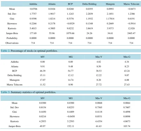
Table 2.Percentage of stocks in optimal portfolios.

MV MG Min-V Min-G

Addoha 0.00 0.00 4.82 4.34

Atlanta 9.91 9.48 8.50 8.23

BCP 46.39 54.77 38.53 43.24

Delta Holding 15.11 12.12 12.22 9.87

Managem 17.07 14.74 8.20 6.88

[image:5.595.85.538.97.517.2]

Maroc Telecom 11.52 8.90 27.72 27.43

Table 3.Summary statistics of optimal portfolios.

MV MG Min-V Min-G

Mean 0.0300 0.0300 0.0068 0.0064

Std. Dev 0.8154 0.8253 0.7565 0.7607

Gini 0.4450 0.4409 0.4118 0.4098

Skewness 0.0216 −0.0450 0.0531 0.0098

Kurtosis 4.2953 5.2593 4.4354 4.8673

Jarque-Bera 49.97 152.11 61.63 103.74

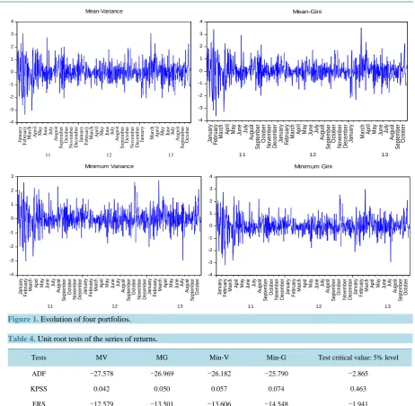
Return series for optimal portfolios are plotted in Figure 1. Plots demonstrate that the return series are extremely unstable.

In order to make the comparison of the two strategies clearer, we used quasi-analytic VaR and CVaR methods using the GARCH (1.1) model, because the variance is not homoscedastic as the ARCH test result proves. This was done in order to take into account those specific characteristics apparent in our data. In order to move away from a normal distribution framework for the prediction of VaR and CVaR, we used the Cornish-Fisher expan-sion and the Johnson SU approximation.

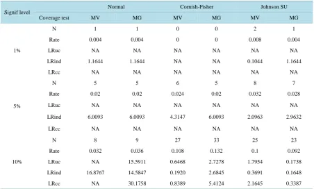
Table 4 presents the different tests of stationary. We accept the alternative hypothesis that the series of returns of the four portfolios are stationary and the result of the ARCH test leads us to reject the null hypothesis. There-fore, it is assumed that the residual variance is not homoscedastic. The prediction the quasi-analytic VaR and CVaR of portfolios will be made on a GARCH (1; 1) model.

4. Results

4.1. Estimating Parameters

(6)

[image:6.595.78.541.76.528.2]

Figure 1. Evolution of four portfolios.

Table 4.Unit root tests of the series of returns.

Tests MV MG Min-V Min-G Test critical value: 5% level

ADF −27.578 −26.969 −26.182 −25.790 −2.865

KPSS 0.042 0.050 0.057 0.074 0.463

ERS −12.579 −13.501 −13.606 −14.548 −1.941

ARCH test 49.848 71.045 41.329 57.636 1.710

point of view, for portfolios in times of market turbulence.Table 5andTable 6 present parameters of GARCH (1.1) Model with Normal Distribution and Student-t Distribution.

4.2. Back-Testing VaR Estimates

We evaluated the accuracy of the proposed VaR estimates over a 250 day period using the now standard coverage tests of Christoffersen (1998). We combined the GARCH (1.1) model with the approximation method. The Cor-nish-Fisher expansion, and the Johnson SU approximation derive the VaR estimates for each portfolio where

10%

α = ; 5% and 1%.

In finance literature tells us that there are two fundamental test procedures used to compare the performances of VaR: Unconditional and Conditional. We make use of Kupiec’s (1995) Test to evaluate GARCH specifications for unconditional coverage, and the Christoffersen Test to embrace both unconditional coverage and the indepen-dence of violations. The Kupiec Test and Christoffersen Test results for the portfolios are reported in Tables 7-10.

-4 -3 -2 -1 0 1 2 3 4 Jan u ar y F eb ru ar y M ar ch Ap ri l Ma y Ju n e Ju ly A ug us t S ep tem b er O ct o b er N o v em b er D ecem b er Jan u ar y F eb ru ar y M ar ch Ap ri l Ma y Ju n e Ju ly A ug us t S ep tem b er O ct o b er N o v em b er D ecem b er Jan u ar y M ar ch Ap ri l Ma y Ju n e Ju ly A ug us t S ep tem b er O ct o b er

11 12 13

Mean-Variance -4 -3 -2 -1 0 1 2 3 4 Januar y F ebr uar y Ma rc h Ap ri l M ay June Ju ly A ugus t S e p te m b e r O ct ober N ov em ber D ec em ber Januar y F ebr uar y Ma rc h Ap ri l M ay June Ju ly A ugus t S e p te m b e r O ct ober N ov em ber D ec em ber Januar y Ma rc h Ap ri l M ay

June Ju

ly A ugus t S e p te m b e r O ct ober

11 12 13

Mean-Gini -4 -3 -2 -1 0 1 2 3 Ja nu ar y F e b ru a ry M a

rch _Apri

l M ay Ju n e Ju ly A ug us t S ep tem ber O ct ob er N o vem ber D e cem ber Ja nu ar y F e b ru a ry M a

rch _Apri

l M ay Ju n e Ju ly A ug us t S ep tem ber O ct ob er

11 12 13

Minimum Variance -4 -3 -2 -1 0 1 2 3 4 Ja nu ar y F e b ru a ry M a

rch _Apri

l M ay Ju n e Ju ly A ug us t S ep tem ber O ct ob er

11 12 13

(7)

Table 5. Estimating parameters of GARCH (1.1) model with normal distribution.

MV MG Min-V Min-G Probability

0

α 0.08663426 0.08924027 0.11720896 0.11712902 0.00

1

α 0.23139483 0.27226848 0.22481727 0.24679101 0.00

1

β 0.64211892 0.59980154 0.56927745 0.54694141 0.00

Table 6. Estimating parameters of GARCH (1.1) model with student-t distribution.

MV MG Min-V Min-G Probability

0

α 0.09442063 0.09672067 0.0940 0.0947 0.00

1

α 0.25967866 0.31700487 0.2327 0.2559 0.00

1

[image:7.595.88.541.283.555.2]

β 0.60933342 0.56057089 0.6099 0.5879 0.00

Table 7. Unconditional coverage and conditional coverage of VaR GARCH (1.1) model with normal distribution.

Signif level

Normal Cornish-Fisher Johnson SU

Coverage test MV MG MV MG MV MG

1%

N 1 1 0 0 2 1

Rate 0.004 0.004 0 0 0.008 0.004

LRuc NA NA NA NA NA NA

LRind 1.1644 1.1644 NA NA 0.1044 1.1644

LRcc NA NA NA NA NA NA

5%

N 5 5 6 5 8 7

Rate 0.02 0.02 0.024 0.02 0.032 0.028

LRind 6.0093 6.0093 4.3147 6.0093 2.0963 2.9632

10%

N 8 9 27 33 25 23

Rate 0.032 0.036 0.108 0.132 0.1 0.092

LRuc NA 15.5911 0.6468 2.7278 1.7954 0.1738

LRind 16.8767 14.5847 0.1920 2.6845 0.3691 0.1648

LRcc NA 30.1758 0.8389 5.4124 2.1645 0.3387

Finally, we utilised CVaR to compare the two pairs of strategies because the outcomes are similar and CVaR can better capture the tail risk. Results are reported in Tables 11-14.

5. Discussion

This paper discusses and compares analytical results obtained with MV, MG, the Min-V and the Min-G strate-gies on the Moroccan financial market (MADEX) during periods of market instability, and demonstrates, em-pirically, that quasi-analytic GARCH VaR forecasts can be accurately constructed using analytic formulae for higher moments of aggregated GARCH returns by using Cornish-Fisher expansion and the Johnson SU distribu-tion.

(8)

[image:8.595.99.537.101.397.2]

Table 8. Unconditional coverage and CONDITIONAL coverage of VaR GARCH (1.1) model with student-t distribution.

Signif level

Coverage test MV MG MV MG MV MG

1%

N 0 0 0 0 2 1

Rate 0 0 0 0 0.008 0.004

LRind NA NA NA NA 0.104431 1.164423

5%

N 6 5 7 7 8 8

Rate 0.024 0.02 0.028 0.028 0.032 0.032

LRind 4.3147 6.0093 2.9632 2.9632 1.9067 1.9067

10%

N 14 13 41 46 25 22

Rate 0.056 0.052 0.164 0.184 0.1 0.088

LRuc 6.2591 9.5052 9.8922 16.3634 0.9614 0.3909

LRind 6.1990 7.5231 9.8791 16.3192 0.0004 0.3890 LRcc 12.4582 17.0283 19.7713 32.6826 0.9618 0.7800

Table 9.Unconditional coverage and conditional coverage of VaR GARCH (1.1) model with normal distribution.

Signif level

Coverage test Min-V Min-G Min-V Min-G Min-V Min-G

1%

N 0 0 0 0 1 2

Rate 0 0 0 0 0.004 0.008

LRind NA NA NA NA 1.1644 0.1044

5%

N 4 4 4 4 14 12

Rate 0.016 0.016 0.016 0.016 0.056 0.048

LRuc NA NA NA NA 0.2557 0.3015

LRind 8.1149 8.1149 8.1149 8.1149 0.1956 0.0173

LRcc NA NA NA NA 0.4513 0.3189

10%

N 13 10 24 24 26 25

Rate 0.052 0.04 0.096 0.096 0.104 0.1

LRuc 7.6730 13.2293 1.1502 0.2691 1.7469 0.1131

LRind 7.5231 12.5238 0.0365 0.0365 0.0533 0.0004

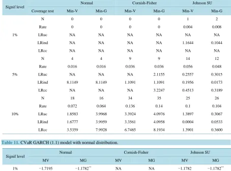
[image:8.595.97.539.422.718.2]

(9)

Table 10.Unconditional coverage and conditional coverage of VaR GARCH (1.1) model with student-t distribution.

Signif level

Coverage test Min-V Min-G Min-V Min-G Min-V Min-G

1%

N 0 0 0 0 1 2

Rate 0 0 0 0 0.004 0.008

LRind NA NA NA NA 1.1644 0.1044

5%

N 4 4 9 9 14 12

Rate 0.016 0.016 0.036 0.036 0.056 0.048

LRuc NA NA NA 2.1155 0.2557 0.3015

LRind 8.1149 8.1149 1.1091 1.1091 0.1956 0.0173

LRcc NA NA NA 3.2247 0.4513 0.3189

10%

N 18 16 34 35 25 26

Rate 0.072 0.064 0.136 0.14 0.1 0.104

LRuc 1.8583 3.9968 3.3924 4.0976 1.3897 0.3067

LRind 1.6777 3.9959 3.3561 4.0958 0.0004 0.0533

[image:9.595.84.539.104.441.2]

LRcc 3.5359 7.9928 6.7485 8.1934 1.3901 0.3600

Table 11.CVaR GARCH (1.1) model with normal distribution.

Signif level

MV MG MV MG MV MG

1% −1.7195 −1.1782** _NA _NA _−1.1782 _−1.1782**

5% −1.7705 −1.4003** _−1.7288 _−1.6720** _−1.5539 _−1.5263** 10% −1.0460 −0.9254** _−1.0460 _−0.9253** _−1.0803 _−1.0059** **

[image:9.595.87.542.514.589.2]

Represent the lower CVaR of both strategies.

Table 12.CVaR (1.1) model with student-t distribution.

Signif level

MV MG MV MG MV MG

1% NA NA NA NA −1.1782 −1.1782

5% −1.7288 −1.6720** _−1.6011 _−1.5263** _−1.5539 _−1.4568** 10% −1.2485 −1.2106** −0.9248 −0.8425** −1.0804 −1.0079** **

[image:9.595.89.539.631.706.2]

Table 13.CVaR GARCH (1.1) model with normal distribution.

Signif level

Min-V Min-G Min-V Min-G Min-V Min-G

1% NA NA NA NA −2.3361 −1.9087

5% −1.4848 −1.4374** _−1.4848 _−1.4374** _−1.1156 _−1.1140** 10% −1.1418** −1.1475 −0.9502 −0.9132** −0.9249 −0.9002** **

(10)

[image:10.595.89.542.102.181.2]

Table 14.CVaR (1.1) Model with student-t distribution.

Signif level

Min-V Min-G Min-V Min-G Min-V Min-G

1% NA NA NA NA −2.3361 −1.9087**

5% −1.4848 −1.4374** _−1.2180 _−1.1648** _−1.1156 _−1.1140** 10% −1.0365 −1.0213** −0.8544 −0.8240** −0.9376 −0.8907** **

CVaR to that of the MV strategy. This is also true of the Min-G strategy in relation to the Min-V strategy. In view of these results, we conclude that the MG strategy outperforms the MV strategy in our real-world examples taken from the Moroccan Financial Market. This is due to the characteristics of the financial assets that do not follow a normal distribution and the unstable nature of the variance in time.

There was great accuracy for all significance levels (10%, 5% and 1%), when we considered for GARCH VaR forecasting. Our results are even more remarkable when we consider that the analysis is entirely out-of- sample and that the testing period (2011-2014) covers several prolonged periods of excessively turbulent finan-cial market activity.

References

Agouram, J., & Lakhnati, G. (2015). Mean-Gini Portfolio Selection: Forecasting VaR Using GARCH Models in Moroccan

Financial Market. Journal of Economics and International Finance, 7, 51-58.

Christoffersen, P. F. (1998). Evaluating Interval Forecasts. International Economic Review, 39, 841-862.

http://dx.doi.org/10.2307/2527341

Dorfman, R. (1979). A Formula for the Gini Coefficient. Review of Economics and Statistics, 61, 146-149.

http://dx.doi.org/10.2307/1924845

Favre, L., & Galeano, J. A. (2002). Mean-Modified Value-at-Risk Optimization with Hedge Funds. Journal of Alternative

Investments, 5, 2-21. http://dx.doi.org/10.3905/jai.2002.319052

Kupiec, P. (1995). Technique for Verifying the Accuracy of Risk Measurement Models. Journal of Derivatives, 2, 173-184.

http://dx.doi.org/10.3905/jod.1995.407942

Markowitz, H. (1952a). Porfolio Selection. Journal of Finance, 7, 77-91.

Markowitz, H. (1952b). The Utility of Wealth. The Journal of Political Economy(Cowles Foundation Paper 57), LX (2),

151-158.

Markowitz, H. (1959). Portfolio Selection: Efficient Diversification of Investments. New York: Wiley.

Shalit, H., & Yitzhaki, S. (1984) Mean-Gini, Portfolio Theory, and the Pricing of Risky Asset. Journal of Finance, 39, 1449-

1468. http://dx.doi.org/10.1111/j.1540-6261.1984.tb04917.x

Shephard, N. (1996). Statistical Aspects of ARCH and Stochastic Volatility. Monographs on Statistics and Applied

Proba-bility, 65, 1-68.

Yitzhaki, S. (1982). Stochastic Dominance, Mean-Variance, and Gini’s Mean Difference. American Economic Review, 2,

178-185.

Zangari, P. (1996). A VaR Methodology for Portfolios That Include Options. RiskMetrics Monitor, JP Mogran-Reuters, First